HAL Id: hal-00426392
https://hal.archives-ouvertes.fr/hal-00426392v2
Submitted on 26 Oct 2009
HAL is a multi-disciplinary open access
archive for the deposit and dissemination of
sci-entific research documents, whether they are
pub-lished or not. The documents may come from
teaching and research institutions in France or
abroad, or from public or private research centers.
L’archive ouverte pluridisciplinaire HAL, est
destinée au dépôt et à la diffusion de documents
scientifiques de niveau recherche, publiés ou non,
émanant des établissements d’enseignement et de
recherche français ou étrangers, des laboratoires
publics ou privés.
Local unified models of backscattering from ocean-like
surfaces at moderate incidence angles
Nicolas Pinel, Christophe Bourlier
To cite this version:
Nicolas Pinel, Christophe Bourlier. Local unified models of backscattering from ocean-like surfaces at
moderate incidence angles. International Radar Conference, Oct 2009, Bordeaux, France. pp.0107.
�hal-00426392v2�
LOCAL UNIFIED MODELS OF BACKSCATTERING FROM
OCEAN-LIKE SURFACES AT MODERATE INCIDENCE ANGLES
Nicolas Pinel and Christophe Bourlier
IREENA Laboratory – Radar Team
Polytech’Nantes, Université de Nantes
Nantes, France
nicolas.pinel@gmail.com
,
christophe.bourlier@univ-nantes.fr
Abstract— In the context of electromagnetic
wave backscattering from ocean-like surfaces, by
using the SSA-1 model, Bourlier et al. proposed
a technique to reduce the number of numerical
integrations to two for easier numerical
implementation. To be consistent with
microwave measurements, closed-form
expressions of the Fourier coefficients of the
backscattering RCS are obtained.
For Gaussian
statistics, previous work is extended to kernels of
unified models expanded up to the order two,
like the SSA2 and LCA2.
Electromagnetic scattering by rough surfaces, Random media, Sea surface, Water pollution, Multistatic scattering
I. INTRODUCTION
From the 1960s, the derivation of the microwave backscattering normalized radar cross section (BNRCS) from ocean surfaces is a topic of investigation which makes progress and remains a challenging task. The first developed model is the TSM [1, 2]. Recently, this approach was improved [3–5]. In the last two decades, another group of scattering models was proposed, namely the local unified models. The term local means that the multiple scattering phenomenon is neglected, and the term unified means that the model satisfies the high- and low- frequency limits, given by the geometric optics approximation (GOA) and the small perturbation method (SPM), respectively. For more details, see the thorough review of Elfouhaily and Guérin [6]. One of the most popular is the SSA2 published by Voronovich [7, 8, 9]; more recently, models based on the same decomposition of the scattering matrix as SSA2, like the LCA2, were published by Elfouhaily et al. [10, 11].
It is well known that such backscattering models are extremely difficult to implement in the full three-dimensional case, because of the four-fold integral that is involved (two space variables and two frequency variables) and because of the strongly oscillating behavior of the integrand. That is why, recently, Bourlier and Pinel presented [12, 13] an original
technique to reduce this computation to a two-fold integral (one space variable and one frequency variable) by resorting to azimuthal harmonic expansion of the BNRCS and by using Bessel functions. This is done for two-harmonic spectra such as the Elfouhaily et al. spectrum [14].
In this paper, this model is presented and tested for microwave frequencies and different wind speeds. The paper is organized as follows. In section 2, the technique developed by Bourlier and Pinel is briefly summarized, and in section 3, the BNRCS is compared with its first order, easier to compute than the second order. The last section gives concluding remarks.
II. BNRCS OF UNIFIED SCATTERING MODELS
In the literature, from microwave (C and Ku bands for
instance) experimental data [15, 16, 17], it was established that
the BNRCS σpq can be expressed for pq={VV,HH}
co-polarizations in the form
where φ is the observation azimuthal angle with respect to the wind direction, θ the observation elevation angle, and u the wind speed. The isotropic backscattering term σ0pq mainly
describes the wind speed, σ1pqthe surface asymmetry between
the up (φ=0) and down (φ=180°) wind directions, and σ2pqthe
surface asymmetry between the up (φ=0) and cross (φ=90°) wind directions. For Gaussian statistics, σ1pq=0. Non-Gaussian
statistics is addressed in [12] by considering only the SSA-1 kernel.
By considering the first two orders of the kernels of unified
models, ,
which depend on the chosen model, the NRBCS is then equal to the sum of two terms, σpq= σ
11pq + σ12pq. The subscript “11”
results from the correlation of the first-order scattered field, whereas the subscript “12” results from the cross-correlation between the first- and second- order scattered fields. The vectors k0 and k (boldface denotes a vector) are the horizontal
components of the incident and the scattered waves (whereas q0 and qk are the vertical ones, see figure 1).
Figure 1. Geometry of the problem
By assuming Gaussian statistics, Bourlier and Pinel [13] recently showed that the BNRCS harmonics
related to “11” can be expressed as
where
and A=1/(πQz2), Qz = 2Kcosθ, kB = 2Ksinθ, K=2π/λ, in which
λ is the radar wavelength. W0(r) and W2(r) stand for the
isotropic and anisotropic parts of the height autocorrelation function, respectively. The hat over W, as a function of ξ, corresponds to the associated spectrum. In polar coordinates
(ξ,φξ), the sea spectrum is assumed to be
, which is consistent with the Elfouhaily et al. sea spectrum [14]. Jm and Im are the
Bessel functions of the first and second kinds, respectively, and of order m. The above equations show that the BNRCS is obtained from a single numerical integration over the radial distance r, instead of two, with one over r and one over an angular variable. Thus, the numerical evaluation of the order “11” is rather simple. For the SSA model, Ν1pq is given by the
SPM model, whereas for the LCA model, it is given by the Kirchhoff approximation model. Their expression can be found in [13].
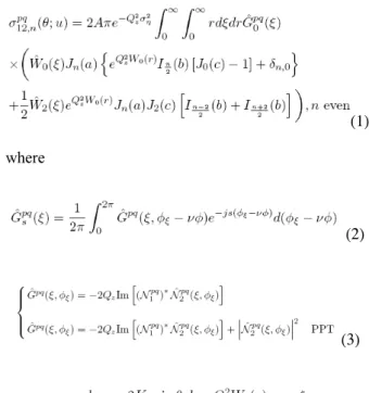
For the LCA2 model, we have (ν=0)
(1) where
(2)
(3)
and δn,m is the Kronnecker Symbol, such that δn,m=1 if n=m ; 0
otherwise.
Equation (2) is the Fourier series of the kernel
expressed from the first- and second-
order kernels. In the backscattering direction, their expression can be found in [13]. To simplify the derivation of the BNRCS, the PPT is often applied, which
implies a new definition of the kernel . Under the
PPT, in Eq. (3), the term is derived from the BNRCS (for instance, see Eqs. (21) and (22) of [13]) by using the series expansion ex ≈ 1+x. By comparison, the scattered field (for
instance, see Eq. (10) of [13]) derived under the PPT uses the reverse way, that is to say the approximation 1+x ≈ ex.
For the SSA2 model, we have (ν=1)
(4) where
and
with real. Unlike the LCA2 model, the SSA2 model
requires the computation of a sum over s. For s=0, corresponding to the LCA2 model, Eq. (1) is found.
The SSA2 requires the computation of a sum because its
second-order sub-kernel depends on the angle φξ,
whereas the LCA2 second-order sub-kernel is isotropic, since it is independent of φ−φξ. This fundamental difference implies
that the derivations led for the SSA2 model are more complicated than that of the LCA2 model. It is also important to note that Eq. (4) is valid for any kernel obeying the same properties as SSA2 or LCA2.
III. NUMERICAL RESULTS
A. Numerical implementation
For incidence angles of interest for remote sensing
applications, θ∈[0;60]°, and for the VV and HH
co-polarizations, this section presents numerical results of the incoherent BNRCS by assuming an anisotropic height spectrum given by the Elfouhaily et al. [14] model. Two radar frequencies are studied, f=5.3 GHz (C-band, sea relative permittivity εr=67+j35 [18]) and f=14 GHz (Ku-band, εr
=47+j38 [18]).
The numerical evaluations of the BNRCSs are rather simple. First, the isotropic W0(r) and anisotropic W2(r) parts of the
correlation function are computed over r ∈[0;rmax]. For
frequencies f={5.3,14} GHz, the maximum radial distance rmax≈{5,1} meters. It decreases when the incidence angle
decreases, the wind speed increases and the frequency increases. It is important to note that since the sea correlation function is independent of {θ,f}, {W0(r),W2(r)} were computed
and stored in a data file. In addition, the sampling over the radial distance r is done in a logarithmic scale with 200 samples.
The numerical evaluations of the BNRCSs are
more complicated, because they require an additional integration over the sea wavenumber ξ∈[ξmin;ξmax]. We choose
ξmin=0.25kp, which corresponds to the value for which the sea
height isotropic spectrum falls down to 10-5 times its
maximum, which occurs at kp. The value ξmax equals 4K. Thus,
the double integration over r ∈[0;rmax] and over ξ∈[ξmin;ξmax],
is done in a logarithmic scale with 200x200 samples. Finally, the Fourier series coefficients defined by Eq. (2) are calculated by using a sampling step over φ−νφξ of 3 degrees. The
BNRCSs require the computation of a sum over s from 0 to smax. With the LCA model, smax=0 whereas for the SSA model,
smax must be determined. This aspect is presented in details in
[13]. It is shown that the integer smax increases slightly with the
angle θ, is few sensitive to the polarization and the order n of the harmonic. Typically, for θ ≤ 30°, smax ≤ 3 whereas for
θ∈]30;60]°, smax reaches the maximum value 7 in average.
Thus, the sum over s converges rapidly.
With these parameters, for a given incidence angle θ, on a PC with 4GB of RAM and a processor of 3 GHz, the computing time is of the order of 0.9 second. The scope of the paper is not to compare the different backscattering models with measurements. This was thoroughly already done in previous works [9, 12, 20].
B. Comparison of SSA2, LCA2 and SPM1
Figures 2 and 3 plot the harmonics of the BNRCS versus the incidence angle θ for f={14, 5.3} GHz, u10=10 m/s and for
VV and HH polarizations. The labels in the legend mean
SSA11 corresponds to computed from the
SSA-1 model with n={0,2} and pq={VV,HH},
SSA11+12 corresponds to computed
from the SSA2 model with n={0,2} and pq={VV,HH},
LCA11 corresponds to computed from the
LCA-1 model with $ n={0,2} and pq={VV,HH}, LCA11+12+PPT corresponds to
computed from the LCA2 model combined with the PPT with n={0,2} and pq={VV,HH},
SPM-1 corresponds to computed with SPM and
given by
As expected, the BNRCS decreases more quickly for HH polarization.
For near-nadir incidence angles, figures 2 and 3 reveal that the LCA11 and the SSA11 models are similar, which means that SSA11 reproduces the KA (Kirchhoff Approximation) reduced to the SPA (stationary Phase Approximation).
Theoretically, SSA11 does not reproduce the KA, but since the sea surface is highly conducting and the backscattering angle vanishes, the SPM polarization matrix is close to the Kirchhoff one.
It can be noted that by construction, the LCA11 model is the same as the KA+SPA model. For incidence angles ranging from 0 to approximately 20 degrees, only the gravity waves contribute to the scattering and therefore the KA+SPA can be applied. However, a smooth transition for scattering angles θ∈ [20;40]° is observed, for which the KA+SPA model becomes invalid and the Bragg scattering regime (given by SPM) contributed increasingly. In this region, SSA11 tends to SPM, and the higher orders of SSA2 and LCA2 contribute. For the LCA2 model, this contribution is positive for the VV polarization, whereas it is negative for the HH polarization. For the SSA2 model, this contribution is negative for the VV polarization and it is weak, whereas it is positive for the HH polarization and it is much smaller than that of the LCA model. Thus, the behavior of the kernel of each model is very different.
It is important to note that the LCA2 results plotted in figures 2 and 3 use the PPT, which consists in adding the term
in Eq. (3). If the PPT is not applied, then for larger scattering angles, simulations not reported in this paper, show a non-physical behavior of the BNRCS for the HH polarization. With the SSA model, the results obtained with the PPT are the same as the ones plotted in figures 1 and 2. For a one-dimensional sea surface, as explained in details in the paper of Bourlier et al. [19], although the LCA kernel reaches the SPM and the KA+SPA limits and is tilt invariant, the BNRCS does not converge toward the Bragg regime. A theoretical explanation in given in the conclusion of [19]. Thus, the use of the PPT in the LCA model allows us to remove this drawback. This is why, in the paper of Mouche et al. [20], the LCA model with the PPT gives satisfactory results on the BNRCS.
C. Optimization of the SSA2 and LCA2 computation
Eqs. (1) and (4) require the computation of two-fold numerical integrations over the radial distance r and the sea wavenumber ξ. First, integrating over r, the resulting integrand depends then only on ξ. Plotting this integrand versus ξ, we observe that two wavenumbers {ξl, ξh} mainly contribute to the scattering process. The first one is defined as ξl=1.66kp (low frequency), in which kp corresponds to the wavenumber for which the sea height isotropic spectrum is maximum. In fact, 1.66kp corresponds to the maximum of the slope isotropic spectrum (heigh spectrum multiplied by ξ2). The second one is
defined as ξh=kB (high frequency). Thus, the second-order BNRCS results from the inteference of two waves of wavenumbers {ξl, ξh}. More precisely, for ξ= ξh, one can observe that the adjacent wavenumbers also contribute to the scattering process, and we show that ξh⇒ ξh ∈[kB−Δξ;kB+Δξ] with Δξ=0.5kB. It is equivalent to multiply the sea spectrum by a pulse function centered around kB and of width 2Δξ.
Figure 4 plots the ratio of the SSA2 model
versus the incidence angle θ, with different choices of the integration over ξ. The labels in the legend mean that
for MP1, ξ=ξl=1.66kp for the integration,
for MP2, ξ=ξh for the integration with a sampling step of 0.1 kB (nξ=11),
for MP3, ξ={ξl, ξh} for the integration,
else ξ∈[0.25 kp;4K] (full spectrum) with nξ=200 (number of samples).
As one can see, for low incidence angles, only the sea wavenumber ξ=ξl contributes to the scattering process, whereas for moderate incidence angles (Bragg regime), both the low- (ξl) and high- frequencies (ξh) contribute. Moreover, the results are very close to that obtained from the full spectrum. Thus, with this new integration, the computing time is reduced to 0.07 second instead of 0.90 second, when the full spectrum is used.
Same simulations done with the LCA2 model and not reported here led to different conlusions. Indeed, the results computed from the LCA2+MP2 model are the same as the ones obtained from the LCA2 (full spectrum) model. This shows that only the high-frequency components of the sea spectrum contribute to the scattering process, unlike the SSA2 model, for which both the low- and high- frequency components contribute.
IV. CONCLUSION
In this paper, closed-form expressions of the Fourier coefficients of the BNRCS were expressed for a Gaussian process. Then, the “11” order, resulting from the correlation of the first-order scattered field, requires two independent numerical integrations over the wavenumber ξ (for the calculation of the height correlation function), and over the radial distance r. The “12” order, resulting from the cross-correlation between the first- and second- order scattered fields, requires two-fold numerical integrations over the radial distance r and over the wavenumber ξ, and one numerical angular integration for the computation of the Fourier series coefficients of the second-order kernel. The SSA2 and LCA2 kernels were tested for microwaves frequencies and different wind speeds. The numerical results showed that the SSA2 and LCA2 have different behaviors, and the correction from the “12” order is larger for the LCA2 model than for the SSA2 model. In addition, an optimization for the numerical integration over ξ was proposed, leading to a computing time of the “12” order less than 0.1 second on a standard office computer for a given wind speed, a given frequency and a given incidence angle.
REFERENCES
[1] B. F. Kur’yanov, “The scattering of sound at a rough surface with two types of irregularity,” Sov. Phys. Acoust., vol. 8, pp. 252-257, 1963. [2] W. Wright, “A new model for sea clutter,” IEEE Trans. Ant. Prop., vol.
16, no. 2, pp. 217-223, 1968.
[3] G. Soriano and C.-A. Guérin, “A cutoff invariant two-scale model in electromagnetic scattering from sea surfaces,” IEEE Trans. Geos. Rem. Sensing Letters, vol. 5, no. 2, pp. 199-203, 2008.
[4] N. Sajjad, A. Kenchaf, A. Coathanay and A. Awada, 2008, “An improved two-scale model for the ocean surface bistatic scattering,”
Paper presented at the International Geoscience and Remote Sensing Symposium, in USA, Boston, MA.
[5] S. Boukabara, L. Eymard, C. Guillou, D. Lemaire, P. Sobieski, and A. Guissard, “Development of a modified two-scale electromagnetic model simulating both active and passive microwave measurements: Comparison to data remotely sensed over the ocean”, Radio Science, vol. 37, pp. 1063, 2002.
[6] T. M. Elfouhaily and C.-A. Guérin, “A critical survey of approximate scattering wave theories from random rough surfaces,” Waves Random Complex Media, vol. 14, no. 4, pp. R1-R40, 2006.
[7] A. G. Voronovich, “Small slope approximation for electromagnetic wave scattering at a rough interface of two dielectric half-spaces,” Waves in Random Media, vol. 4, no. 3, pp. 337-367, 1994.
[8] A. G. Voronovich, Wave scattering from rough surfaces. Germany: Springer series on Wave Phenomena (Second edition), 1999.
[9] A. G. Voronovich, “The effect of the modulation of Bragg scattering in small-slope approximation,” Waves in Random Media, vol. 12, pp. 341-349, 2002.
[10] T. M. Elfouhaily, S. Guignard, R. Awadallah and D. R. Thompson, “Local and non-local curvature approximation: a new asymptotic theory for wave scattering,” Waves Random Complex Media, vol. 13, no. 4, pp. 321-337, 2003.
[11] T. M. Elfouhaily and J. T. Johnson, “Extension of the local curvature approximation to third order and full tilt invariance,” Waves Random Complex Media, vol. 16, no. 2, pp. 97-119, 2006.
[12] C. Bourlier, “Azimuthal harmonic coefficients of the microwave backscattering from a non-Gaussian ocean surface with the first-order SSA model,” IEEE Trans. Geos. Rem. Sensing, vol. 42, no. 11, pp. 2600-2611, 2004.
[13] C. Bourlier and N. Pinel, “Numerical implementation of local unified models for backscattering from random rough sea surfaces,” Waves in Random and Complex Media, vol. 19, no. 3, pp. 455-479, 2009. [14] T. Elfouhaily, B. Chapron, K. Katsaros and D. Vandemark, “A unified
directional spectrum for long and short wind-driven waves”, J. Geo. Res., vol. 102, no. C7, pp. 781-796, 1997.
[15] F. J. Wentz, S. Peteherich and L. A. Thomas, “A model function for ocean radar cross section at 14.6 GHz,” J. Geo. Res., vol. 89, pp. 3689-3704, 1984.
[16] A. Bentamy, P. Queffeulou, Y. Quilfen and K. Katsaros, “Ocean surface wind fields estimated from satellite active and passive microwave instruments”, IEEE Trans. Geos. Rem. Sens., vol. 37, pp. 2469-86, 1999.
[17] A. A. Mouche, D. Hauser, J.-F. Daloze and C. Guerin, “Dual-polarization measurements at C band over the ocean: Results from airborne radar observations and comparison with ENVISAT ASAR data,” IEEE Trans. Geos. Rem. Sens., vol. 43, no. 4, pp. 753-769, 2005. [18] W. Ellison, A. Balana, G. Delbos, K. Lamkaouchi, L. Eymard, C.
Guillou, and C. Prigent, “New permittivity measurements of seawater,'' Radio Science, vol. 33, pp. 639–648, 1998.
[19] C. Bourlier, N. Déchamps and G. Berginc, “Comparison of asymptotic backscattering models (SSA, WCA, and LCA) from one-dimensional gaussian ocean-like surfaces,” IEEE Trans. Ant. Prop., vol. 53; no. 5, pp. 1640-1652, 2005.
[20] A. A. Mouche;, B. Chapron and N. Reul, “A simplified asymptotic theory for ocean surface electromagnetic wave scattering,'' Waves Random Complex Media, vol. 17, pp. 321-341, 2007.
0 5 10 15 20 25 30 35 40 45 50 55 60 -35 -25 -15 -5 5 15
Incidence angle θ (degrees)
B N R C S ( d B) VV, n=0 0 5 10 15 20 25 30 35 40 45 50 55 60 -35 -25 -15 -5 5 15
Incidence angle θ (degrees)
B N R C S ( d B) HH, n=0 0 5 10 15 20 25 30 35 40 45 50 55 60 -35 -25 -15 -5 5 15
Incidence angle θ (degrees)
BN R C S ( d B) VV, n=2 0 5 10 15 20 25 30 35 40 45 50 55 60 -35 -25 -15 -5 5 15
Incidence angle θ (degrees)
BN R C S ( d B) HH, n=2 SSA11 SSA11+12 LCA11 LCA11+12+PPT SPM-1
Figure 2. Harmonics of the BNRCS versus the incidence angle θ for f=14 GHz, u10=10 m/s, VV (left) and HH (right) polarizations and for n={0 (top), 2
0 5 10 15 20 25 30 35 40 45 50 55 60 -35 -25 -15 -5 5 15
Incidence angle θ (degrees)
BN R C S ( d B ) VV, n=0 0 5 10 15 20 25 30 35 40 45 50 55 60 -35 -25 -15 -5 5 15
Incidence angle θ (degrees)
BN R C S ( d B ) HH, n=0 0 5 10 15 20 25 30 35 40 45 50 55 60 -35 -25 -15 -5 5 15
Incidence angle θ (degrees)
BN R C S ( d B) VV, n=2 0 5 10 15 20 25 30 35 40 45 50 55 60 -35 -25 -15 -5 5 15
Incidence angle θ (degrees)
BN R C S ( d B) HH, n=2 SSA11 SSA11+12 LCA11 LCA11+12+PPT SPM-1
Figure 3. Same as in Figure 2 but for f=5.3 GHz.
0 5 10 15 20 25 30 35 40 45 50 55 60 0 0.1 0.2 0.3 0.4
Incidence angle θ (degrees)
Ra ti o |σ 12 |/σ 11 VV, n=0 0 5 10 15 20 25 30 35 40 45 50 55 60 0 0.1 0.2 0.3 0.4
Incidence angle θ (degrees)
Ra ti o |σ 12 |/σ 11 HH, n=0 0 5 10 15 20 25 30 35 40 45 50 55 60 0 0.1 0.2 0.3 0.4
Incidence angle θ (degrees)
Ra ti o |σ 12 |/σ 11 VV, n=2 0 5 10 15 20 25 30 35 40 45 50 55 60 0 0.1 0.2 0.3 0.4
Incidence angle θ (degrees)
Ra ti o |σ 12 |/σ 11 HH, n=2 SSA11+12 SSA11+12 +MP1 SSA11+12 +MP2 SSA11+12 +MP3