Article
Site Amplification Analysis of Dushanbe City Area, Tajikistan
to Support Seismic Microzonation
Farkhod Hakimov 1,2,3,*, Gisela Domej 4, Anatoly Ischuk 1, Klaus Reicherter 2, Lena Cauchie 3
and Hans‐Balder Havenith 3 1 Seismic Hazard Assessment Department, Academy of Sciences, Institute of Geology, Earthquake Engineering and Seismology, Aini Street 265, Dushanbe 734060, Tajikistan; anatoly.ischuk@gmail.com 2 Neotectonics and Natural Hazards, RWTH Aachen University, Lochnerstraße 4–20, 52056 Aachen, Germany; k.reicherter@nug.rwth‐aachen.de 3 Geology Department, University of Liège, Allée du 6 Août, 14/B18, 4000 Liège, Belgium; lena.cauchie@uliege.be (L.C.); hb.havenith@uliege.be (H.‐B.H.) 4 Dipartimento di Scienze dell’Ambiente e della Terra, Università degli Studi di Milano–Bicocca, Piazza della Scienza 1/U4, 20126 Milano, Italia; gisela.domej@unimib.it * Correspondence: farkhod.hakimov@doct.uliege.be Abstract: Being a country exposed to strong seismicity, the estimation of seismic hazard in Tajikistan
is essential for urbanized areas, such as the rapidly growing capital city Dushanbe. To ensure people’s safety and adequate construction work, a detailed seismic microzonation is the key to proper hazard planning. Existing estimations of seismic hazard date back to 1978; they are based on engineering geological investigations and observed macroseismic data. Thereupon relies the Tajik Building Code, which considers seismic intensities according to the Medvedev–Sponheuer– Karnik Scale, MSK‐64. However, this code does not accurately account for soil types, which vary considerably in Dushanbe—not only by their nature, but also due to increasing anthropogenic influences. In this study, we performed a series of analyses based on microtremor array measurements, seismic refraction tomography, and instrumental data recording from permanent stations for standard spectral ration and from mobile seismic stations for the horizontal to vertical spectral ratio in order to provide a comprehensive full‐cover microzonation of Dushanbe accounting for soil types. Our results identify several critical areas where major damage is likely to occur during strong earthquakes.
Keywords: ambient noise measurements; seismic refraction tomography; instrumental data
recording; site effect; soil characteristics; borehole data; microzonation 1. Introduction Similar to other big agglomerations in Central Asia (such as the Uzbekistan capital Tashkent or the Kyrgyzstan capital Bishkek), Dushanbe with its outskirts (Figure 1a,b) is at particular risk from earthquakes and the associated secondary hazards due to its close vicinity to two active fault systems. The Hissar–Kokshaal Fault passes some 10–15 km north of the city, and the Ilyak–Vaksh Fault crosses at about 20–25 km in the south. For both fault systems Babaev et al. [1] estimate maximum Mw magnitudes of 7.5 and 6.5, respectively (see Figure 1).
First reliable earthquake records in Tajikistan date back to the 1895s. Since that time more than 20 earthquakes with magnitudes equal or greater than 7.0 have occurred [2]. Among the latter, the Karatag Earthquake in 1907 (Mw = 7.4), the Sarez Earthquake in 1911 (Mw = 7.4) and the Khait Earthquake in 1949 (Mw = 7.4) can be cited as examples for catastrophic events [3], although not for Dushanbe (Figure 1). Citation: Hakimov, F.; Domej, G.; Ischuk, A.; Reicherter, K.; Cauchie, L.; Havenith, H.‐B. Site Amplification Analysis of Dushanbe City Area, Tajikistan to Support Seismic Microzonation. Geosciences 2021, 11, 154. https://doi.org/10.3390/ geosciences11040154 Academic Editors: Jesus Martinez‐ Frias and Giovanni Barreca Received: 15 February 2021 Accepted: 28 March 2021 Published: 31 March 2021 Publisher’s Note: MDPI stays neutral with regard to jurisdictional claims in published maps and institutional affiliations.
Copyright: © 2021 by the authors. Licensee MDPI, Basel, Switzerland. This article is an open access article distributed under the terms and conditions of the Creative Commons Attribution (CC BY) license (http://creativecommons.org/licenses /by/4.0/).
A more recent and also very damaging earthquake near Dushanbe was located in the Tajik Depression in South‐Western Tajikistan (Figure 1)—the Hissar Earthquake on 22 January 1989 (Mw = 5.8). With a very shallow depth of about 5 km, the intensity degree VII (i.e., “very strong”) on the Medvedev–Sponheuer–Karnik Scale (MSK‐64; [4]) was reached in the settlement of Hissar causing small direct damage on buildings, but triggered extensive liquefaction phenomena and related landslides in loess deposits. The villages of Sharora and Okuli‐Poen were affected by mudflows destroying more than 100 houses, and 247 persons died. At a distance of 13 km from Dushanbe, the Hissar Earthquake was felt with an intensity of V units (i.e., “fairly strong”) according to the MSK‐64 scale [5].
Figure 1. Study Area: Location of Tajikistan in Central Asia and the extent of the capital Dushanbe. The red circles show
historical earthquakes, and the yellow circles show local earthquakes used in this study. The red lines show the most important seismogenic faults. Faults mentioned in the text are labeled.
For seismic hazard assessment, seismic sources located at different distances from Dushanbe are of particular interest. The highest hazard arises from earthquakes within a radius of 30–50 km and at depths of 5–30 km ([6]). As proposed by Babaev et al. [1], there is indeed a strong probability of occurrence of such events within the mentioned radius for example along the closely located Hissar–Kokshaal Fault. An intensity of IX units (i.e., “destructive”) on the MSK‐64 scale resulting from such close and shallow earthquakes could be reached at different places throughout Dushanbe [7]. The fact that the ground beneath the city consists mainly of different types of sediments and sedimentary rocks plays here an important role, as the material tends to amplify and prolong the seismic shaking, and, thus, enhances the hazard potential. This latter phenomenon is known as “site effects”. Remote earthquakes beyond the mentioned radiuses, for instance from the Pamir‐ Hindukush Subduction Zone, may become dangerous if they develop great magnitudes, and if the duration may be about one or even several minutes. The results might be vibratory motions with specifically unfavorable spectral compositions, which can spread
over vast areas and become a danger for high buildings. Intensities could reach up to VI units (i.e., “strong”) on the MSK‐64 scale [8]. Even though the need of detailed seismic hazard assessment in Tajikistan is apparent, studies on the area are sparse. Only recently, intensity assessments for Central Asia were proposed by Bindi et al. [9], and Pilz et al. [10] evaluated the seismic risk for Dushanbe. Additionally, some neighboring regions were studied [11]. On a global scale, a seismic hazard map was made available by the Global Seismic Hazard Assessment Program (GSHAP; [12,13]) on which peak ground accelerations (PGAs) of 0.40–0.48 g (= 3.92–4.71 m/s²) are assigned to Western Tajikistan; PGA values of 0.38–0.40 g (= 3.73–3.92 m/s²) were estimated by Ischuk et al. [14] for Dushanbe. However, so far there was no comprehensive full‐cover microzonation available for Dushanbe in particular—a fact that our site characterization study should remedy.
Considering the fast expansion of Dushanbe entailing new high rise constructions, seismic hazard maps should incorporate two main aspects. On one hand, maps must reflect the seismic activity potential and ground motions in terms of one or more parameters—in terms of intensities according to the MSK‐64 scale, and in the terms of accelerations (PGA—peak ground acceleration). On the other hand, the local soil response to seismic impacts must be considered in order to provide accurate maps, which could subsequently be used for hazard mapping and during the development of a more accurate seismic building code.
Typical for most urbanized areas is a dense agglomeration inducing a wide range of conditions and disturbing factors, which limit the application of many geophysical methods that allow for complex seismic microzonation. In many cases, invasive methods (e.g., drilling and borehole measurements) are impossible to implement [15]. For this reason, only non‐invasive methods were used for data acquisition (Table 1): microtremor array measurements (MAMs), seismic refraction tomography (SRT), and instrumental data recording from temporary and permanent and from mobile seismic stations for long‐ and short‐term acquisition, respectively. The use of these methods individually or in combination has proven to be successful for detailed seismic characterization and microzonation in the past (e.g., [10,16–26]). The newly assessed data was combined with local geological and geotechnical data in the form of lithological maps and cross sections as well as borehole logs provided by the Head Institute of Engineering and Technical Surveys of the State Construction Committee of Tajikistan (HIETSCCT; [27]).
Table 1. Non‐invasive methods used for the collection of new data. Compiled data (*) from the Head
Institute of Engineering and Technical Surveys of the State Construction Committee of Tajikistan (HIETSCCT; 2019) were evaluated and adapted to meet the requirements of our study.
Method Assessed Data Processing Results
175—Horizontal to Vertical Spectral Ratio (HVSR) measurements passive vibration (ambient noise at 30‐min intervals) Horizontal to Vertical Spectral Ratio (HVSR) Fundamental Resonance Frequency Map 9—Seismic Refraction Tomography (SRT) profiles active vibration (P‐wave) P‐wave inversion P‐wave velocity (Vp) patterns, subsurface structures 5—Microtremor Array Measurements (MAM) passive vibration (ambient noise at two‐ hour intervals) Spatial Autocorrelation (SPAC), Rayleigh Wave Dispersion curves, S‐wave velocity (VS) patterns 5—temporary seismic stations recordings & 1 permanent reference station passive vibration (instrumental data) Standard Spectral Ratio (SSR) from earthquake Amplification factors data compilation (*) lithological maps and cross sections data of 60 boreholes (data evaluation and adaption) Surface lithology, subsurface structures
2. Local Geology and Previous Microzonations Dushanbe is located at the foot of the Hissar Range in an east–west trending valley with the same name and about 70 km long and 20 km width. The main river in the Hissar Valley is the Kafirnigan River flowing westwards; first and second order tributaries are the Varzob River and the Luchob River and the Hissar Canal (Figure 2a). The planes to both sides of the Kafirnigan and the Varzob Rivers are covered with extensive layers of alluvial and proluvial deposits; thus, Dushanbe is built on those quaternary sedimentary sequences consisting of gravel and sand alternating with layers of loam soils and loess (Figure 2a). Figure 2. (a) River system and lithology in the area of Dushanbe (after [28]) and (b) seismic microzonation of Dushanbe by [29] based on the acoustic stiffness of the soils in terms of the MSK‐64 scale.
Quaternary sediments and sedimentary rock reach depths of up to 300 m. The chronologically older Paleogene sedimentary rocks beneath have thicknesses of 600 m to 1400 m; and Upper and Lower Cretaceous sedimentary rocks are believed to be between 600 and 900 m thick. In total, thus, Meso‐ and Cenozoic deposits extend to about 3 km in depth [30–33]. Mesozoic and tertiary rocks consist mainly of sandstone, but also to large parts of conglomerates, clays, limestone, and gypsum. Sandstone is present beneath almost all parts of Dushanbe under the uppermost gravel and loess covers (see above in Figure 2a); the only sandstone outcrops are found in the north across flanks bordering the Varzob and Luchob Valleys.
The major part of the city is located on three terraces and partly on the adjoining foothills (regionally termed in Central Asia, “adyrs”—are hill sloping foothills and individual hills and ridges on the valleys’ slopes) and on diluvial terrain at altitudes of 800–900 m above sea level. The Varzob River floodplain starts with a narrow valley in the north, gradually expands southwards following the Varzob River, and consists mainly of gravel with embedded sand layers and greater boulders. This sequence of deposits is found likewise beneath the second and the third terraces in Dushanbe area. Thicknesses generally decrease from about 300 m in the center of Dushanbe and the right bank of the
Varzob River towards the north, west, and east thinning out to thicknesses of only 20–40 m. The second terrace, called Hissar Terrace, rises with a 1–3 m high cliff above the Varzob flood‐plain. It consists on average of 5–10 m thick loess covers. Additionally, the third terrace comprises mainly loess layers with an average thickness of 10–30 m and a cliff of 12–18 m towards the second terrace. With a gradient of 3% it is slightly inclined towards the southwest (see the cross section in Figure 3c). The outskirts of Dushanbe show complex geological structures, which are still poorly explored—even to a depth of several tens of meters.
Water supply to the city and its population resulted in a large number of boreholes drilled in Dushanbe. Data from boreholes is a valuable resource that helps with the interpretation of the passive seismic surveys and allows one to obtain various preliminary cross section of the sedimentary cover from southwest to northeast (Figure 3c). Borehole data and lithological cross section were collected from the Head Institute of Engineering and Technical Surveys of the State Construction Committee of Tajikistan (HIETSCCT; [27]) and a previous study of [29] to support the mapping of the lithological units across Dushanbe, the delineation of underground layer sequences and subsurface structures within the sedimentary soils and, finally, the interpretation of the results of the applied geophysical methods. In total, 60 boreholes were drilled to depths of 30–200 m across the city (Figure 3).
In terms of tectonics, Dushanbe is located in an area affected by strong seismicity regularly experiencing shallow (focal depths ≤45 km) and deep (focal depths ≥ 70 km) earthquakes. The frequency of medium to strong events is shown in Figure 4, in which epicenters of earthquakes from the Central Asia Seismic Risk Initiative, Earthquake Modeling for Central Asia Catalogue (CASRI‐EMCA; [34,35]) over the period from 850 to 2015, and updated from USGS catalogue (U.S. Geological Survey) over the period from 2015 to 2020. Strong earthquakes in Western Tajikistan with magnitude 4.5 ≤ M ≤ 8.2 are shown in Figure 4. Western Tajikistan is crossed by several major faults and subfaults. Two of the major faults are located in close vicinity to Dushanbe: the Hissar–Kokshaal Fault in the north and the Ilyak–Vaksh Fault in the south with our estimation of possible maximum magnitudes (Mw) of 7.6 and 7.5, respectively (see Figure 1). In an earlier study with the aim of a general seismic zonation of Dushanbe, Babaev et al. [8] hypothesized that the city could experience intensities with up to IX units (i.e., “destructive”) on the MSK‐64 scale. The zonation is still in use as a reference for the seismic building code in Tajikistan. The earliest seismic zonations date back to the 1930s, and were based on soil types [36]. A combined work of Nazarov and Nechaev [37], Kogan et al. [38], and Oripov [39] consist of two separate zonations with intensity from VIII units (i.e., “damaging”) to >IX units (i.e., “destructive) on the MSK‐64 scale for buildings with less and more than five floors, respectively. Both seismic zonations are the basis for the Tajik Seismic Building Code currently in use. The latest seismic zonation was established by [29] based on the two separate zonings and use the same partition of intensity units (Figure 2b).
Figure 3. Locations of 60 boreholes, 5 microtremor array measurements (MAM), 9 seismic refraction tomography (SRT) profiles, 5 temporary seismic stations for standard spectral ratio (SSR) measurements, and 175 mobile seismic stations for horizontal to vertical spectral ratio (HVSR) measurements (a). The permanent seismic station Djerino (DZET, located in (b) serves as reference and is installed on a granite bedrock outcrop some 14 km north of Dushanbe (maps with hill shade and colored shuttle radar topography mission digital elevation model, SRTM DEM, of 30 m resolution as the background). Lithological cross section cutting through Dushanbe from southwest to northeast along profiles sketched from available boreholes (c); after the Head Institute of Engineering and Technical Surveys of the State Construction Committee of Tajikistan [27,29]. The numbers in the cross section (c) indicate examples of borehole logs (Section 4.1). The first step towards an area‐wide site characterization based on soil response was carried out by Pilz et al. [10] within the framework of the regional program “Earthquake Modeling for Central Asia” (EMCA) by the Global Earthquake Model Foundation (GEM Foundation), which emphasizes the refinement of existing seismic hazard maps for cities in Central Asia. Considering the complex sequence of lithology and the thereby entailed
significant lateral and vertical variations of soil properties, the authors underlined the need for a new assessment of seismic risk based on site effects and the vulnerability of the buildings. A dense seismic network allowed for the assessment of amplification patterns and shear wave velocity (VS) gradients, whereas single‐station noise measurements shed light on ground motion variability. Remote‐sensing data delivered additional information on the vulnerability of the building stock. However, with the steadily growing number of (also large) buildings constructed on a layered sequence of sedimentary deposits favoring the amplification and the prolongation of vibratory motion, a detailed seismic zonation of Dushanbe is essential. This study provides new inputs for a future microzonation based on a multimethodological approach.
Figure 4. Epicenters of shallow (focal depths ≤ 45 km; marked in red) and deep (focal depths ≥ 70 km; marked in blue)
earthquakes from the Central Asia Seismic Risk Initiative, Earthquake Modeling for Central Asia Catalogue (CASRI‐ EMCA; [34,35]) over the period from 850 until 2015, and updated from USGS catalogue (U.S. Geological Survey) over the period from 2015 until 2020.
3. Applied Geophysical Methods
In order to better understand the local seismic response of the different soil types and subsurface structures, the following non‐invasive seismic methods were conducted: five microtremor array measurements (MAM), nine seismic refraction tomography (SRT) profiles, five temporary seismic stations for standard spectral ratio (SSR) measurements with one permanent station serving as reference, and 175 horizontal to vertical spectral ratio (HVSR) measurements (Table 1). The results of recent measurements were combined with lithological maps, cross sections and data from 60 borehole logs [27]. Figure 3 presents an overview of the locations of new investigations and the boreholes. All methods were completed between 2018 and 2020, and borehole log from 1965 to 2019.
3.1. Horizontal to Vertical Spectral Ratio (HVSR) Measurements from Mobile Seismic Stations Originally, the method of measuring the horizontal to vertical spectral ratio (HVSR) from ambient noise or passive vibration input was popularized by [40] and largely used for two decades. Nakamura [40] described that the HVSR between horizontal and vertical ambient noise records is related to the fundamental resonant frequency (natural frequency) of the soil (f0) when a sedimentary deposits lies over bedrock. This method involves evaluating the ratio of the amplitude spectra obtained from the horizontal and vertical components of the seismometer [41]; results characterize the frequency spectra in terms of resonance and predominant frequencies [42]. The method is widely used in site effect assessments and in geotechnical studies [43–45]. The most common field of application is seismic microzonation of urban areas (e.g., [17,19–21,24,46]).
A total of 175 ambient noise recordings were carried out throughout Dushanbe (located in the map in Figure 3) using a mobile Mark L‐4C‐3D seismometer with a resonance frequency of 1 Hz connected to an EarthData PR6‐24 recorder with GPS timing. At each site, ambient noise was recorded during 30 min at a rate of 100 samples per second (100 Hz) for statistical signal stabilization. In addition, the azimuth of each peak was estimated to calculate the HVSR in all orientations of the horizontal plane.
Almost all measurements were placed directly on soils or gravel; only a few measurements were made on tarmac. To ensure sufficient accuracy, the measurements have never been carried out in critical weather conditions (i.e., with rain and/or strong wind) as recommended by the ‘Site Effects Assessment using Ambient Excitations’ (SESAME) project [47]. Most of the ambient noise recordings were made in the central, northern, and eastern parts of the city with an interval of at least 500 m between each other, while some specific recording sites were selected to cover typical topographic areas, such as, for example, mountain slopes, river junction, or free fields (Figure 3a).
3.2. Seismic Refraction Tomography (SRT)
The seismic refraction tomography (SRT) is a common method to assess the P‐ and S‐wave velocities of soils, and is widely used in the field of geotechnical engineering [48– 51]. The frequent usage of SRT is owed to its simplicity, flexibility, and rapidity; the limitation of investigations to depths of several tens of meters could, however, be regarded as drawback. By applying inversion methods (i.e., either P‐ and/or S‐wave inversions) on SRT profiles, P‐ and/or S‐wave velocity patterns within the underground are obtained, which shed light on subsurface structures.
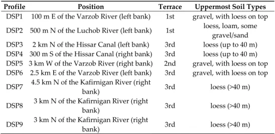
In order to assess the seismic soil properties, we performed nine SRT in zones of different building densities throughout Dushanbe, each of which had a length of 115 m (DSP1–DSP9 in Figure 3; Table 2). Active vibratory input was recorded in the form of P‐ waves using 24 geophones sensitive to 4.5 Hz and spaced at intervals of 5 m, all of which were connected to a 16‐bit Geometrics ES‐3000 Seismograph. Seismic impacts were generated on the ground surface by club hammer strokes on a metal plate at five different positions relative to the aimed seismic profile: one at each profile end, one in between, and two with an offset of 25 m in straight prolongation to the profile. All profiles were orientated roughly in the north–south direction. Table 2 provides information on the location, position relative to the three terraces and prevalent soil types visible from the surface. Recorded data was processed with the software SARDINE [52] in 2D after picking P‐wave arrival times manually. In order to ensure correct wave propagation within a half‐ space, the minimum and maximum expected P‐wave velocities (Vp) were limited to 300 m/s (for air) and 4000 m/s (for hard sandstone), respectively. P‐wave inversion was carried out using the simultaneous iterative reconstruction technique (SIRT; [53]) implemented in SARDINE.
Table 2. Seismic refraction tomography (SRT) profiles with details on location, position relative to
the three terraces and prevalent soil types visible from the surface.
Profile Position Terrace Uppermost Soil Types
DSP1 100 m E of the Varzob River (left bank) 1st gravel, with loess on top DSP2 500 m N of the Luchob River (left bank) 1st loess, loam, some gravel/sand DSP3 2 km N of the Hissar Canal (left bank) 3rd loess (up to 40 m) DSP4 300 m S of the Hissar Canal (right bank) 3rd loess (up to 40 m) DSP5 3 km W of the Varzob River (right bank) 2nd gravel, with loess on top DSP6 2.5 km E of the Varzob River (left bank) 3rd gravel, with loess on top DSP7 4.5 km N of the Kafirnigan River (right bank) 3rd loess (>40 m) DSP8 3 km N of the Kafirnigan River (right bank) 3rd loess (>40 m) DSP9 3 km N of the Kafirnigan River (right bank) 3rd loess (>40 m) 3.3. Microtremor Array Measurements (MAMs) Ambient noise measurements have proven useful for 2D and 3D seismic subsurface characterizations to derive shear wave velocity (VS) patterns within the underground [54– 58]. Being a passive method, it is particularly suitable for the evaluation of site effects and subsequently of the seismic hazard [16,43]. Usually, frequencies ranging from 1 to 25 Hz are recorded capturing mainly ambient noise induced by human activity (e.g., traffic or heavy machinery) and natural phenomena (e.g., wind or water courses); this noise is referred to as microtremor ([59]).
Microtremor array measurements (MAMs) allow us to identify of the phase velocities of surface waves (vertical components of the Rayleigh Waves were mainly analyzed). Via the method of spatial autocorrelation (SPAC; [60–63]), dispersion curves of Rayleigh Wave phase velocities are obtained and then processed through surface wave inversion to compute the 1D (vertical) shear wave velocity (VS) distribution of the underground. Dispersion curves are commonly shown in graphs plotting shear wave velocities (VS) as a function of wavelengths (or frequencies). MAM with resulting vertical shear wave velocity (VS) variations are representative for a single location bounded by the array polygon.
In this study, we established five MAM in the eastern (DA1 and DA2), the southern (DA3 and DA4) and the western (DA5) parts of the city (DA1–DA5 in Figure 3; Table 3). For this purpose, we used five three‐component Trillium Compact 20s Seismometers connected to a 24‐bit DATA‐CUBE3 Recorder in a pentagonal geometry configuration without an additional central sensor. The radius of the MAM usually varied between 45 and 50 m depending on the location. Record durations lasted for two hours for each MAM with a sampling rate of 100 Hz. For all MAM, only vertical components were used for processing Rayleigh Waves from ambient noise. Table 3. Microtremor array measurements (MAM) with details on location, position relative to the three terraces, and prevalent soil types visible from the surface.
Array Position Terrace Uppermost Soil Types
DA1 3.5 km N of the Kafirnigan River (right bank) 3rd loess (>40 m) DA2 3.3 km N of the Kafirnigan River (right bank) 3rd loess (<40 m) DA3 1.5 km W of the Varzob River (right bank) 2nd gravel DA4 3.2 km W of the Varzob River (right bank) 3nd gravel DA5 700 m N of the Hissar Canal (left bank) 3rd loess (<40 m)
3.4. Standard Spectral Ratio (SSR) Measurements from Temporary Seismic Stations
Earthquake shaking has been recorded over a period of five months at five temporary seismic stations in the city and at one permanent seismic station located on a granite outcrop some 14 km north of Dushanbe serving as reference (located at “SSR” points in the map in Figure 3). For the five locations within the city, Trillium Compact 20s Seismometers were used connected to a 24‐bit DATA‐CUBE3 Recorder. The reference station in Djerino (DZET; Figure 3b) is equipped with a CMG‐3ESPC Seismometer connected to a Güralp CMG‐DM24—6 Channel Recorder. Table 4 provides information on the location, position relative to the three terraces and prevalent soil types visible from the surface.
The spectral amplitudes were calculated by the reference site method, more precisely by the standard spectral ratio method (SSR; [64]), by comparing the record of earthquakes in the study area with the records of the nearby reference station. Records from the reference site (station placed on the rock) are assumed to contain the same sources and effects on propagation as records from other sites [10,24,65]. This ratio can be calculated for all three components separately, i.e., vertical (Z), north–south (N), and east–west (E), but it mostly applies to the average horizontal spectra (e.g., [23,45,66,67]). The spectral ratio can therefore directly deliver the site response [22,45,65,66].
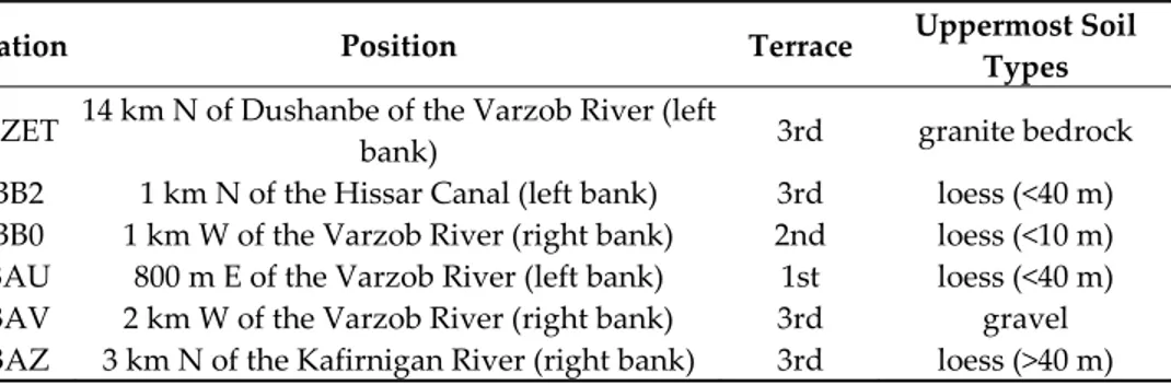
Table 4. The temporary seismic stations for standard spectral ratio (SSR) with details on location,
position relative to the three terraces and prevalent soil types visible from the surface.
Station Position Terrace Uppermost Soil
Types
DZET 14 km N of Dushanbe of the Varzob River (left
bank) 3rd granite bedrock
BB2 1 km N of the Hissar Canal (left bank) 3rd loess (<40 m) BB0 1 km W of the Varzob River (right bank) 2nd loess (<10 m) BAU 800 m E of the Varzob River (left bank) 1st loess (<40 m) BAV 2 km W of the Varzob River (right bank) 3rd gravel BAZ 3 km N of the Kafirnigan River (right bank) 3rd loess (>40 m)
4. Data Processing and Results
4.1. Comparison of the Borehole Data
The seismic properties of soils are assessed in terms of seismic velocities (Vp and VS) and other physical characteristics and their geological and geomorphological position. The properties of gravels are slightly variable. As for loess soils, their features depend on their geological and geomorphological position and are highly susceptible to changes due to anthropogenic factors.
The velocity of S‐waves for loess in Dushanbe varies considerably, although the average characteristics are often close to VS = 235 m/s [29]. Higher values of the parameter are typical of loess soils developed on terraced surfaces and lower values are typical of the adyrs.
We compare the estimated lithological cross‐section from southwest to northeast with existing borehole data (see Figure 3c). In the geotechnical map in Dushanbe [28], lithological profiles’ cross‐sections were included (see Figure 3a). Based on the map, the cross‐section A–B (Figure 3c) is compared with the use example at six sites information of the borehole data. Figure 5 compares the borehole data with inverted Vs profiles from downhole data of the previous studies by [29]. The depths of the borehole data and Vs profile are up to 100 m. Based on the borehole data, the soil in the south‐west of the city is composed of thin layers of loess, gravel deposits, and conglomerate in the lower layers. In the center of the profile, according to the borehole data, the soil consists of gravel deposits, and conglomerates made of lime cement and rocks in the lower layers. In the
north‐eastern part, the total thickness of loess deposits within the study area varies, according to drilling and geophysical data, from 40 to 120 m at the junction of the foothill plain with a high terrace and to 160–200 m at the adyrs. Vs profiles, which correspond to gravel deposits, ranges from 380 to 550 m/s and for conglomerate from 600 to 750 m/s [29]. Figure 5. The borehole and downhole logs of the invasive technique based on the study of [29] allowed the determination of the shear‐wave velocity profile with depth VS of the cross‐section cutting through Dushanbe from west to east (Figure 3c). 4.2. Results of the Seismic Refraction Tomography (SRT) Profiles According to the estimated SRT profiles from nine locations (DSP1–DSP9 in Figure 6), the subsurface structures can be grouped into four classes of different P‐wave velocities <750 m/s, 750–1250 m/s, 1250–2500 m/s, and 2500–4000 m/s. Each of them is representative for different lithological layers: (i) loess layers with different thicknesses and degrees of compactness, (ii) gravel with embedded boulders and sand fillings, (iii) conglomerates (possibly intact rock), and (iv) sandstone bedrock. This link to lithological layers is supported by comparison with borehole data (Figure 3).
The uppermost layer with P‐wave velocities <750–1250 m/s corresponds to the second and third terraces’ uppermost loess layers (Figure 6). SRT profiles DSP2, DSP3, and DSP4 in the northwestern part of the city show loess layers with a thickness of 30–35 m, whereas in the northeastern part close to the foothills, SRT profiles DSP7, DSP8, and DSP9 were made on top of loess layers extending over more than 40 m in depth. On SRT profiles, DSP1 and DSP6, loess layers with a thickness of 5–10 m can be outlined. The next layer, 1250 < Vp < 2500 m/s, has a thickness between 10 and 15 m on profiles DSP3, DSP4, DSP5, DSP8, and DSP9, while on profiles DSP1 (north) and DSP6 (southeast) the thickness of this layer was 30 m and more (Figure 6). This layer can be defined as the thickness of gravel deposits with boulders, which is supported by existing the borehole data (Figure 3). Additionally, on these profiles DSP5, DSP6, and DSP9, we could observe at larger depth a velocity of 2500 < Vp < 4000 m/s with a thickness between 5 and 10 m. This layer is most likely made of conglomerate rocks. On the other hand, in the northern part of the
city, the DSP1 profile shows a relatively large skewed layer, marked 2500 < Vp < 4000 m/s, which approached the top layer of the SRT profile had a thickness between 10 and 35 m. According to the geology of the northern region, where the Varzob Mountain Range begins, this P‐wave velocity of the DSP1 profile represents a sandstone layer (Figure 6).
Figure 6. Results of the nine seismic refraction tomography (SRT) profiles, dash white line showed basis of loess layer. 4.3. Results of the Horizontal to Vertical Spectral Ratio (HVSR) Measurements from Mobile Seismic Stations
The analysis of the HVSR ambient noise data was conducted using the Geopsy software (Available online: http://www.geopsy.org/download/archives/geopsypack‐src‐ 3.3.3.tar.gz (accessed on 20 October 2019); [68]). In this analysis, the signal from the ambient noise measurement is represented by the signal amplitude of the three components recorded over time. Each signal component is then subdivided into a series of time windows with a length of 8–30 s. The Fourier spectra amplitudes of the three components were subsequently computed and smoothed smoothing parameter of 40 by the Konno and Ohmachi [69] function.
The data were analyzed over a frequency range of 0.5–25 Hz and the measured HV peaks were identified following the recommended criteria for clarity and reliability in accordance with the SESAME project [47].
A total of 175 ambient noise measurements were analyzed, and for each of them the HVSR with fundamental resonance frequency (f0) and peak amplitude (A0) were obtained. The second or third peaks were designated as f1 and f2 and amplitude A1 and A2, respectively. The fundamental resonance frequency (f0) observed by HVSR curves corresponded to the geological characteristics of the subsurface layer [40,45,70,71]. Therefore, the peak frequency is an important indicator of the interface of geological features and layers.
From 175 measurement points, we obtained 90 curves with a clear single peak, 26 curves with multiple peaks, and 14 curves with double peaks. We also identified 45 flat peaks associated with gravel deposits in Southern and Southwestern Dushanbe. Comparing the HVSR peaks with geological and borehole data revealed the consistency of the peaks with the soil layers.
A high frequency peak (10.8 Hz) was observed in the northern part of the city, suggesting a very thin layer of soft sediment laying over the hard rocks (Figure 7(D50)). On the northwest part of the city, similar high frequency peak (8–10 Hz) was also encountered on alluvial deposits, which were made of gravel of varying degrees of compaction (Figure 7(D52)). Both of the measurement points D50 and D52 had their loess layer close to the surface at depths of 10–12 m depth.
The HVSR results show that D111 and D61 had a clear peak in range of 1 Hz and 1.5 Hz (Figure 7(D61,D111)), which corresponded to the depth of the loess layer, which we could also observe in the lithological settings map. According to the map D111 was located at adyr hills where the depth of the loess was above 40 m and D61 was located at the foot of the hill where the depth of the loess was up to 40 m. Both D76 and D146 curves had flat curve with low amplitude spectra without clearly identified peak. In the map they correspond to the south and south‐west sites in the base of the city that shows clearly a rock response of alluvial deposits that were made of conglomerate and gravel materials (Figure 7(D76,D146)).
The north‐western part of the city shows a high amplitude peak at frequencies varying from 2 to 4 Hz (Figure 7(D69,D73)). The differences of the f0 and A0 of D69 and D73 could be linked to the variable thickness of loess sediments, which in case of the D69 was located at the depth of 35 m and for D73 had a depth from 25 to 15 m. Both of these HVSR results had a clear peak. The upper quaternary and recent deposits alluvial gravels, conglomerates, loess were characterized by intermediate fundamental frequencies (6–17 Hz) and lower amplitude with an almost flat curve (seen example in Figure 7(D78,D146)). As the amplitude often remained below 2, the peak amplitude rarely fulfilled the SESAME [47] reliability criterion.
Multiple HVSR peaks were often observed in urban areas, where the local lateral variations due to complex subsurface formations cause peak broadening (Figure 7(D117)) or multiple peaks (Figure 7(D42)) due to Rayleigh wave refraction [17]. HVSR curves with double peaks (Figure 7(D11,D112)) on the north‐east and east site of the city at the proximity of the adyr hills corresponded to the multiple layers due to the delluvial terrain. The first peak with a frequency range of 0.8–1 Hz was the fundamental frequency f0, which was supported by HVSR peaks from other measurement points on the adyr hills. The second peak f1 with a frequency range of 4–5 Hz was suggested to be the delluvial terrain, as indicated by the lithological settings.
Figure 7. Selected examples of horizontal to vertical spectral ratios (HVSRs) curves showing clear peak (D50, D52, D61, D69, D73, and D111), double peak (D11 and D112) and multiple peaks (D42 and D117) with examples of flat HVSR curves that show a small peak (D76 and D146). The HVSR plot is represented by a thick black continuous line as the averaged HVSR curve, black dashed lines as HVSR standard deviation (std), its associated peak amplitude HVSR (A0) with std, f1 as secondary peak frequency of amplitude. In Figure 8, the HVSR results are represented through a combined form of lozenge shape: the frequency value is marked by the color of the lozenge, the associated amplitude by its size and the preferred azimuth of the shaking by the orientation of the long diagonal. The 1D‐measurements with clear double frequency peaks are displayed as super‐imposed lozenges (the peak of smaller amplitude being on top).
Figure 8. Results of the horizontal to vertical spectral ratios (HVSRs) analyses. Colors of lozenges indicate five different
classes of fundamental frequency (f0), the sizes of lozenges show the peak amplitudes (A0), and the orientation of the long
diagonals represents the azimuths.
4.4. Results of the Microtremor Array Measurements (MAMs)
In September 2019, five MAM measurements using five seismic stations, which were installed in various parts of Dushanbe (see locations in Figure 9) to obtain information on local shear‐wave velocity patterns.
Seismic noise from surface measurements consists of surface waves, and the inversion of the Rayleigh dispersion curve represents the shear wave velocity profile. Only the vertical components of ambient noise recordings were used in the calculations. The records were prepared for instrumental processing, taking into account the calibration parameters of each sensor, and the results were analyzed using SPAC analysis and inverted by using a neighborhood algorithm [72]. The models obtained from the inversion of dispersion curves show shear wave velocities from 0 to 80 m (Figure 9). Supported by lithological evidence, the Vs of 200–250 m/s obtained at DA5 in the top 45 m suggests the presence of loess materials (Figure 9, map). Furthermore, we observe that Vs increased from 250 to 450 m/s, which defines the compact layer of the gravel at depths of 45–80 m. For the DA4 array, we observe an onset of Vs 400 m/s on the uppermost layer, which increased to 550 m/s up to 25 m depth. This velocity at the beginning may refer to the mixed loess and gravel layer, which then increased, going deep into the gravel layer. The
second shear wave velocity profile of 550–700 m/s at depths from 25 to 65 m indicates the gravel layer with a higher degree of compaction. Further, at a depth of 65–80 m, the velocity profile accelerated from 700 to 1250 m/s, which may indicate the presence of bedrock (conglomerate or sandstone).
In the case of the DA3 array, which is also located on gravel deposits, up to a depth of 25 m there is a shear‐wave velocity profile of 420 m/s. In addition, when moving deeper, the velocity profile gets higher from 420 to 600 m/s at depths of 25–55 m, which suggests a higher degree of compaction of gravel. At the depth above 55–80 m the shear wave velocity Vs gets up to 1200 m/s, which suggests the presence of sandstone or conglomerate (Figure 9). DA1 and DA2 arrays were located on the east side of the city and are located on the loess layers. Shear wave profiles of both show similar pattern. At DA2 onset of the Vs was at 200–250 m/s up to 35 m depth. From 35 to 60 m depth the Vs stayed constantly at 310 m/s. At a depth above 60–80 m velocity abruptly increased to 480 m/s, which indicates change of the layer from loess to gravel. A similar low velocity profile (180–240 m/s) was observed at the onset up to 35 m of depth in the DA1 array. From a 35 to 80 m depth a constant velocity profile of 280 m/s stayed, which suggests a higher degree of compaction of the loess layers (Figure 9). Figure 9. Inversion results of five microtremor array measurements (MAMs) and dispersion curves (black lines) and
theoretical curves corresponding to the tested models (color indicates the misfit value). Shear‐wave velocity models for each tested site. The best model achieved is highlighted in red.
4.5. Data Processing of the Earthquake Data
During the period from August 2019 to January 2020 in total 15 earthquakes with magnitude 2.0 < M < 5.3 were registered at five temporary seismic stations in the city and at one permanent seismic station (Figure 3) and analyzed with the use of the Geopsy software by [68].
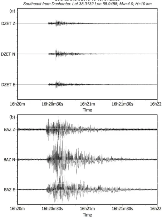
For the higher signal amplitudes and longer duration, we selected 5 over the 15 events with M ranging from 4.0 to 5.3 and with epicentral distance between 30 and 150 km (estimated using the SeisComp3 software). Table 5 presents a list of all events detected during the registration period. An example of the earthquake of 15 October 2019 at 4:20:20 pm (UTC) with the epicenter of the M = 4.0 was 30 km southeast from Dushanbe at the station BAZ (east part of the Dushanbe), and at reference station, DZET is shown in Figure 10. The comparison of both recordings shows that the BAZ station was affected by larger shaking amplitude (here, the amplitude scales are the same for all recordings) than the DZET station, which was actually on the bedrock. Seismogram analysis at the other four stations of the same event shows that BAU and BB2 stations registered higher amplitudes and longer durations than the stations BB0 and BAV (see Figure A1 in the Appendix A). Each seismogram provides data of three components. Table 5. List of the five earthquakes used for the standard spectral ratio (SSR) calculations. Epicenters had a maximum distance of 150 km to Dushanbe.
Year Month Data Time (UTC) Latitude Longitude Magnitude Depth (km)
2019 9 3 4:34:35 PM 38.9476 70.533 4.2 12
2019 9 21 11:30:58 AM 38.6512 70.1729 4.6 21
2019 10 15 4:20:20 PM 38.3132 68.9488 4.0 10
2019 11 12 2:01:49 PM 37.7933 69.9641 4.3 10
2020 1 29 9:10:46 AM 38.8107 70.5587 5.3 10
The standard spectral ratio method (SSR, see, e.g., [10,22–25,67]) involves the comparison of earthquake recordings from nearby sites, using one of them as a reference. As a result, the standard spectral ratio can directly demonstrate the site effect. Reference site choice is generally made with the consideration of seismic velocities and characteristic amplitudes of the different sites. Djerino (DZET), a permanent station located on outcrops of Paleozoic rocks (granite) about 14 km north of Dushanbe, was used as a reference station to calculate the SSR based on its use as a reference site in previous studies of the city [10].
In order to calculate the SSR curves of the five preselected earthquakes, S‐wave windows extracted and a Fourier amplitude spectrum (FAS) was calculated for each of the components. Only the north–south and east–west components were selected to estimate the SSR curve, and each of them was divided by the corresponding component from the reference station (DZET) calculated in a similar way. The resulting SSR curves are illustrated in Figure 11a1–e1. In addition, the squared mean (Havg) was calculated for all horizontal components of the station.
In addition, we calculated the HVSR earthquake curves (EHVSR; Figure 11(a2–e2)) for each station, and the HVSR curves for each station not covering the earthquake period, which represent the HVSR noise (NHVSR; Figure 11(a3–e3)) data. For EHVSR, the S‐wave windows were taken from seismograms with a 5% taper and window length selected consistently with the S‐wave signals’ maximum time duration.
Figure 10. Examples of triaxial seismograms (E for E‐W, N for N‐S, and Z for vertical) for one of the five events recorded at
reference station DZET (a); on rock and BAZ (b); on loess. The epicenter of the 4.0 event is 30 km southeast from Dushanbe. Amplitude scales are the same for all records.
Figure 11. The SSR calculated for the S‐wave window (a1–e1) from five selected earthquakes for the east–west and north– south components at each station and the corresponding spectrum at the DZET (reference station). In addition, (a2–e2) show the HVSR earthquake (EHVSR) curves and (a3–e3) show the HVSR noise (NHVSR) curves from each station. In all figures, the black dashed curve shows the average SSR for the east–west and north–south components for five selected earthquakes. Please note the different amplitude range variation for the station BAZ (c1). 4.6. The Standard Spectral Ratio (SSR) and S‐Waves Results The BAU station data (Figure 11(a1–a3)) show similar patterns of peak activity in the range from 0.5 to 1 Hz and second more prominent peak from about 3 to 6 Hz with an amplitude of 4–6 for the earthquake data (SSR for the E and N components, EHVSR). In addition, a small bump can be observed at the lower frequency range of 0.5–1 Hz in the NHVSR data and clear peak at 4–4.5 Hz. The peak activity at lower frequencies in the SSR and EHVSR curves can be explained by the resonance effect, which may arise from a deeper, more compact layer that can be bedrock (conglomerate or sandstone) and result from S‐waves propagating from the earthquake source.
The BAV station is located on gravel, which can be also confirmed in SSR and EHVSR curves by the absence of the peak at the higher frequencies, which was clearly seen in the SSR and EHVSR curves of the BAU station that is located on a layer of loess (Figure 3). In addition, HVSR peaks from measurement points around the station all show flat curves with a bump at lower frequencies (0.8–2 Hz) which support that BAU station is located on the more compact gravel layer (Figure 3). In the SSR curves of the BAV station we do not observe clear peaks at higher frequencies that are present in the EHVSR curve with a higher amplitude peak. At lower frequencies we observe a peak with high amplitude only on the north component of the SSR (Figure 11(b1–b3)). The EHVSR curves of the BAV and BAU stations both show similar peak activity, which may be due to the same underlying bedrock structure going through both stations. This suggestion can also be supported by the presence of the peak activity at low frequencies of HVSR at the BAV station and only a low amplitude bump at the same frequencies in the BAU station. The BAZ station is located on the thick layer of loess and contains multiple peaks at lower frequencies (0.4–1 Hz) for both north and east SSR curves, EHVSR and NHVSR curves. A similar pattern can be observed from the measurement points of the mobile station HVSR analysis in the proximity of the station (see Figure A2 in the Appendix A). The HVSR peaks around the stations have multiple and single peaks at low frequencies (0.8–2 Hz). SSR curves of north and east components show multiple peaks at lower frequencies ranging from 0.4 to 2 Hz with high amplitudes from 8 to 15. At a frequency range of 2–4 Hz there are observable peaks with lower amplitudes in East SSR, North SSR, EHVSR, and as a bump in the NHVSR. In the NHVSR curve a clear narrow peak at 0.9 Hz can be seen. Peak activity that can be observed in SSR curves and EHVSR at 2–4 Hz can suggest that layer at this range has higher degree of compaction (Figure 11(c1–c3)). Similarly, station BB2, located on the opposite side from station BAZ, is also located on the loess layer (Figure 3). A clear peak of activity can be observed at 1.5 Hz with amplitude 5 in the NHVSR curve, which also supports the presence of a thick loess layer. Comparison with borehole data in the vicinity of the station can show that the loess layer is 40–45 m thick and even thicker near the adyr hills and includes layers of underlying gravel. Therefore, a similar pattern with multiple peaks at lower frequencies (0.5–2 Hz) but with lower amplitudes (6–9 East SSR; 5–6 North SSR) can be observed for the SSR curves. The EHVSR curve shows a clear peak at 1.5 Hz with amplitude 4–5 (Figure 11(e1–e3)). Station BB0 is located on a thin layer of loess (5–10 m) overlying a gravel layer (Figure 3). Therefore, it shows a similar peak pattern with the BAV station, which is also located on gravel. The SSR curves show low amplitude peaks at a frequency range of 0.6–1 Hz with an amplitude ranging from 2 to 4. In addition, a slight increase of amplitude over the frequency range of 4–6 Hz can be observed in the SSR curves, which was amplified in the EHVSR curve with amplitude from 3 to 6. In the NHVSR curve a small narrow peak at 6 Hz with amplitude 2.5 demonstrates that it is located on the thin loess layer (Figure 11(d1– d3)). A comparison with borehole data and cross sections in the proximity of the station confirms the presence of the thin upper loess layer, gravel, and conglomerate layers (Figure 3).
5. Discussion
A geophysical–seismological and geological survey was completed in order to characterize the near‐surface layers and related site effect potential of Dushanbe city and surrounding areas in Tajikistan.
The results of the present analysis based on geological and seismological data, including borehole logs, cross‐sections, HVSR, SRT, MAM, and SSR measurements revealed four distinguishable layers of soil in the area—loess, gravel, conglomerate, and sandstone (bedrock), which were obtained from the areas surrounding the city from the northwest, east, southwest, and southeast. The summarized results and findings for each region are discussed in detail below.
5.1. North and Northwest Territories of Dushanbe City
The P‐wave velocities obtained by the SRT method for the northern DSP1 site (within the valley) quickly increase with a depth up to 4000 m/s on the north side but remain quite low in the southern part, thus indicating a steep south‐dipping bedrock surface at depth (Figure 6). DSP2, DSP3, and DSP4 profiles, which had all been completed in the northwestern zone, all show the same pattern with a lower P‐wave velocity near the surface due to the dominance of the loess layer, which is also confirmed by the borehole data. This P‐wave velocity only increases at a larger depth (>30 m), where the loess is replaced by gravel. In addition, shear wave velocities obtained from the MAM confirm this pattern (Figure 9(DA5)) by lower Vs in the upper layers related to the loess (from 0 to 45 m depth) and Vs increased below 45 m, suggesting the presence of gravel underlain by bedrock at a depth of 80 m.
Site response data obtained from the seismic station BB2 located in the northwestern zone are all marked by a high amplification factor due to the contrast of impedance between the loess and the underlying gravel layers (confirmed by nearby borehole information). This is supported by HVSR measurements from mobile stations located near the station, which showed clear peaks at frequencies of 1–2 Hz (see Figure A2 in the Appendix A, ex: D60, D63). EHVSR curves and NHVSR from the station also show a clear peak in this frequency range. Therefore, the site effects measured in the northwestern zone are expected to be high. 5.2. West and Southwest Side of Dushanbe City P‐wave velocity profiles from DSP5 (located on the west from the BAV station) show the transition from lower velocities (750–1250 m/s) in the upper layer (10–15 m, possibly made of loess) to larger Vp of 2250 m/s at a depth of 20 m to 3500 m/s at a depth of 50 m (Figure 6). The first increase of Vp was related to the gravel’s presence and the second layer of the conglomerate. This is confirmed by the cross‐section data from southwest to the northeast in Figure 6.
Results of DA4 and DA3 arrays, located on gravel, distinguish two groups of soil layers according to Vs profiles, with an upper layer Vs of 400–700 m/s indicating the presence of soft rock and a deeper layer with Vs 1200–1250 m/s representing the harder rock. In the case of DA4, Vs with 1200–1250 m/s starts at a depth of 65 m, and for DA3, it was found below 55 m (Figure 9(DA3,DA4)). This deepening of the top of the conglomerate in the southwestern direction can also be confirmed by the cross‐section data in that zone (Figure 3c).
Site response data from the BAV (southwest) and BB0 (west) stations show very low susceptibility to site amplification. HVSR curves from stations and HVSR curves obtained from the mobile stations in the proximity of those stations all show flat curves characteristic of a low impedance contrast in the subsurface (see Figure A2 in the Appendix A, ex: D62, D54). At both stations, N‐S SSRs show slightly higher site amplification potential within a frequency range of 0.6–1 Hz, marked by amplitudes of 3– 5. The NHVSR curve shows a narrow peak at 6 Hz with an amplitude of 2, which may be due to a thin layer of loess (5–10 m). However, the BAV station did not show any peak within this frequency range. Within the lower frequency range of 0.6–1 Hz, a clear peak is present in both stations’ NHVSR curves (Figure 11(b1–b3,d1–d3)). 5.3. East and North‐East of Dushanbe City P‐wave velocity profiles of DSP7, DSP8, and DSP9 located on the east side of the city all show predominantly low Vp (500–750 m/s) down to a depth of 30–40 m; Vp close to 1250 m/s was only reached at a depth of 50 m for DSP7, and 30 m for DSP8 and DSP9 (Figure 6). On DSP9, at a depth of 50–60 m, the high Vp of 2500–3500 m/s suggests the presence of the gravel layer at this depth. According to the P‐wave data, the uppermost
layer consists of loess. The same soft uppermost layer of loess was suggested by the low shear‐wave velocities measured by the MAM (Figure 9(DA1,DA2)). The two stations BAU and BAZ are located in this area. HVSR measurements near the BAZ station show clear peaks with high amplitude between 0.8 and 2 Hz (see Figure A2 in the Appendix A, ex: D101, D110), whereas HVSR curves near the BAU station show single peaks at a higher frequency of 2.1–4 Hz (see Figure A2 in the Appendix A, ex: D38, D116). The SSR curves from both stations show peaks within a similar frequency range (0.8–2 Hz), but with different amplitude, those at BAZ being clearly larger than those at BAU station (Figure(11a1–a3,d1–d2)). This is also supported by lithological settings, which show that the BAZ station was located on a loess layer that was more than 40 m thick (for BAU, the combined loess and gravel layers could explain the similar amplified frequency range due to a combined larger thickness, but marked by lower amplitudes due to an average larger Vs compared to the pure loess layer in BAZ).
6. Conclusions
The specific and validated seismic hazard assessment for the cities with high infrastructure industry and the population is extremely important. Such a task is particularly important for a city such as Dushanbe, as it is located in a region of high seismicity. The morphology and position of the underlying rocks (depth from the surface), covered by different soft sediments with variable thickness, have previously not been studied sufficiently to be able to provide the information for a reliable seismic microzonation of the urban areas. The same is true for the variability affecting the physical properties of the soils, considering their distribution over the whole area and over different depths. This study is the first one to use four modern seismological methods and data processing techniques to clarify the impact of different ground conditions in Dushanbe on seismic actions. Here, the geophysical–seismological data are presented and analyzed with respect to their geological relevance.
In terms of geophysical and seismic data, this study makes a valuable contribution to assessing seismic hazard and vulnerability in this area. The resulting data that we acquired are highly important for the new seismic microzonation of the city, because existing map of microzoning was made in 1975 based mostly on the engineering‐ geological data. Detailed seismic hazard map for the city can be developed, which then can be used to clarify the seismic actions to the buildings, lifelines, and community planning. Used instrumental methods to define the seismic conditions of the subsurface layers in the Dushanbe city allow one to prepare more accurate and correct seismic microzoning map for improving the aseismic design for new construction in Dushanbe, where the 16‐ and 20‐stores building are the majority of the construction. Additionally, it is clear that the aseismic design of such building must be based on the new methodology and approaches.
An upcoming paper will determine more quantitatively the site effect potential through numerical modeling results; also site effect distribution maps will be presented on the basis of survey and modeling inputs. Thus, these results can be used as inputs for 2D numerical modeling, 3D geomodeling, and will be a basis for further studies, like for the quantitative assessment of seismic impacts on buildings, dams, slopes, and so on. Author Contributions: Conceptualization, H.‐B.H., A.I., and F.H.; Methodology, H.‐B.H., A.I. and
F.H.; Validation, F.H. and H.‐B.H.; Formal Analysis, F.H. and H.‐B.H.; Investigation, F.H.; Resources, A.I., and F.H.; Data Curation, F.H. and A.I.; Writing—Original Draft Preparation, F.H.; Writing—Review and Editing, A.I., G.D., K.R., L.C. and H.‐B.H.; Visualization, F.H. and G.D.; Supervision, H.‐B.H., A.I., and K.R. All authors have read and agreed to the published version of the manuscript.
Funding: This research received no external funding. Institutional Review Board Statement: Not applicable.
Informed Consent Statement: Not applicable.
Data Availability Statement: Unless specified differently, data and imagery used for this
publication are freely available from the following providers or software: ALOS World 3D—30 m (AW3D30)/Credit: JAXA/EORC (Available online: https://www.eorc.jaxa.jp/ALOS/en/aw3d30/index.htm (accessed on 10 September 2019)); ArcGIS/Credit: Esri (version 10.5.1); GEOPSY/Credit: owner (version 3.3.3. Available online: http://www.geopsy.org/download/archives/geopsypack‐src‐3.3.3.tar.gz (accessed on 20 October 2019)); Google Earth Pro/Credit: Google 2020 (version 7.3.3); SRTM 1 Arc‐Second Global/Credit: USGS (Available online: https://earthexplorer.usgs.gov (accessed on 7 September 2019)).
Acknowledgments: We are grateful to the editors and two anonymous reviewers for their
constructive comments, which significantly improved the manuscript. We express our acknowledgments to the German Academic Exchange Service (DAAD) for financial support for the research project in the RWTH Aachen University in the period 2018–2019. The authors also thank to the Department of Neotectonics and Natural Hazards RWTH Aachen University. We are thankful to the technical staff Umedzhon Sharifov, Bekhruz Alamov, Damir Baygenov, and Nusratulo Sharipov of the Institute of Geology, Earthquake Engineering and Seismology of the Academy of Sciences of the Republic of Tajikistan for their help during the field work. We also thank Makhdi Narzulloev and Yakov Andrushuk of the Southern Geophysical Expedition of the Main Department of Geology under the Government of Tajikistan for their instrumental support with the seismic refraction tomography and measurements. Finally, we thank Pulat Aminzoda, Director of the Institute of Geology, Earthquake Engineering and Seismology of the Academy of Sciences of the Republic of Tajikistan, for support and provided instruments for the microtremor measurements in the city area. Conflicts of Interest: The authors declare no conflicts of interest. Appendix A Figure A1. Examples of triaxial seismograms (E for E‐W, N for N‐S, and Z for vertical) for one of the five events recorded at other four stations (BAU, BB2, BB0, and BAV). The epicenter of the 4.0–event is 30 km southeast of Dushanbe.