PASCAL DUBÉ
GEOSTATISTICAL ANALYSIS
OF THE TROILUS DEPOSIT
UNCERTAINTY AND RISK ASSESSMENT
OF THE MINE PLANNING STRATEGY
Mémoire présenté
à la Faculté des études supérieures de l’Université Laval dans le cadre du programme de maîtrise en génie des mines
pour l’obtention du grade de Maître ès sciences (M.Sc.)
DÉPARTEMENT DE GÉNIE DES MINES, DE LA MÉTALLURGIE ET DES MATÉRIAUX
FACULTÉ DES SCIENCES ET DE GÉNIE UNIVERSITÉ LAVAL
QUÉBEC
2006
Résumé
Ce mémoire étudie l’effet de l’incertitude locale et spatiale sur les réserves du gisement d’or Troilus. Deux méthodes géostatistiques ont été utilisées, soit le krigeage des indicatrices et la simulation séquentielle des indicatrices.
En premier lieu, une nouvelle interprétation géologique du gisement a été faite basée sur les trous de forage d’exploration. Pour chaque zone définie, une série de variogrames ont été calculés et un modèle de bloc a été interpolé par krigeage des indicatrices. La calibration de ce modèle a été faite en le comparant au modèle basé sur les trous de forage de production et aux données actuelles de production.
L’incertitude reliée à la variabilité de la minéralization a été quantifiée par l’entremise de 25 simulations séquentielles. Une série de fosses optimales basées sur chaque simulation ont été réalisées afin d’analyser l’impact sur la valeur présente nette, le tonnage de minerai et le nombre d’onces d’or contenues.
Abstract
This thesis examines the effect of local and spatial uncertainty of the mineral reserves estimates for the Troilus gold deposit. Two geostatistical methods have been used: indicator kriging and sequential indicator simulation.
A new set of geological envelope has been defined based on the grade distribution of the exploration hole samples. For each zone, composites, statistics and variograms have been calculated based on gold assays coming from exploration holes (DDH) and production blastholes (BH). A recoverable reserve block model based on indicator kriging was created from the exploration holes and a grade control block model was produced from the production blastholes. The recoverable reserve model was calibrated based on the grade control model and the data from the mined out part of the orebody.
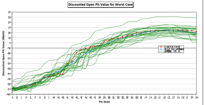
Uncertainty related to the variability of the mineralization was assessed through 25 conditionally simulated block models. Open pit optimization Whittle software was used as a transfer function to compare each model. Elements such as ore tonnage, grade, ounces contained and discounted value (NPV) have been used to analyse the risk inherent to each model. Finally, reserve estimates within an already established pit design were used as a second method of comparison.
Acknowledgements
First and foremost, I would like to express my gratitude to Dan Redmond, for his input, advice, guidance and for always answering my numerous questions during the preparation of this thesis.
I gratefully acknowledge the support of Inmet Mining to pursue this study and the support of my colleague David Warren and Bruno Perron at Troilus Mine.
I would also like to thank Alain Mainville, Manager of Mining Resources & Methods at Cameco Corporation and Professor Kostas Fytas from Université Laval for their comments and time spent reviewing this thesis.
And finally, I would like to thank Mélanie, for her kindness, patience and understanding during my studies.
Table of Contents
CHAPTER 1 Introduction...10
1.1 General introduction ...10
1.2 Description of geostatistics ...2
1.2.1 Introduction...2
1.2.2 Geostatistics and mining ...2
1.2.3 History of geostatistics...4
1.3 Computer software...5
1.4 Troilus Mine...7
1.4.1 Location ...7
1.4.2 Historic of Troilus...8
1.5 Problematic and objectives ...10
CHAPTER 2 Geology...12
2.1 Introduction...12
2.2 Regional and local geology...12
2.3 Troilus deposit...13
2.3.1 Geology and alteration...13
2.3.2 Mineralization ...15
2.3.3 Structure and foliation...17
2.3.4 In-situ density...18
2.4 Conclusion ...18
CHAPTER 3 Geological Modelling ...19
3.1 Introduction...19
3.2 Database ...19
3.2.1 Diamond drill hole (DDH)...19
3.2.2 Blasthole (BH) ...20
3.2.3 Review ...20
3.3 Geological interpretation...21
3.3.1 Definition ...21
3.3.2 Problematic and avenue ...21
3.4 Contact profile analysis...25
3.4.1 Definition ...25
3.4.2 Application...25
3.5 Conclusion ...27
CHAPTER 4 Compositing...28
4.1 Introduction...28
4.2 Diamond drill holes (DDH) ...28
4.2.1 Sample data and composite statistics ...28
4.2.2 Compositing variance ...29
4.3.1 Sample data statistics ...30
4.4 Data set comparison ...31
4.6 Conclusion ...34
CHAPTER 5 Spatial Continuity Analysis ...35
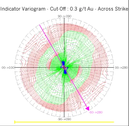
5.1 Introduction...35 5.2 Contour map...35 5.3 Variography ...36 5.3.1 Description...36 5.3.2 Data transformation...38 5.3.3 Indicator transformation...38 5.3.4 Indicator cut-off ...42 5.3.5 Indicator variogram...43 5.4 Conclusion ...47
CHAPTER 6 Reserve Estimation ...48
6.1 Introduction...48 6.2 Interpolation method ...48 6.2.1 Selection method...48 6.2.2 Method selected ...49 6.3 Indicator kriging...49 6.3.1 Pros...49 6.3.2 Cons ...50 6.3.3 Implementation ...50 6.4 Block size...52 6.5 Block model ...52 6.6 Reconciliation ...53 6.6.1 Data provided...53 6.6.2 Mineable packet ...53
6.6.4 Discussion and analysis ...58
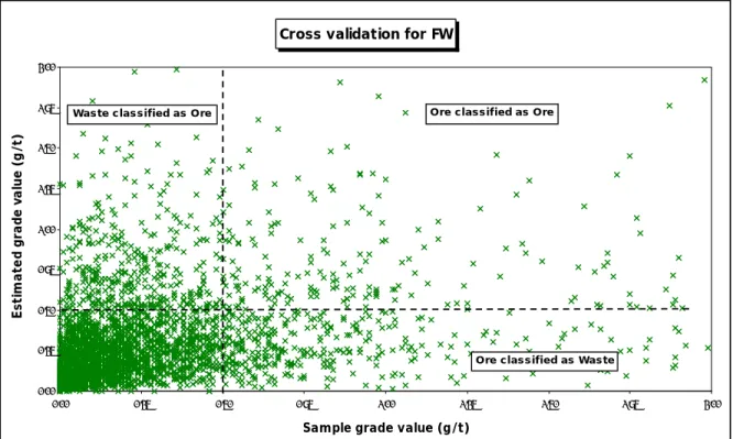
6.7 Cross validation...59
6.7.1 Introduction...59
6.7.2 Limitation...59
6.7.3 Misclassification ...60
6.8 Conclusion ...64
CHAPTER 7 Conditional Simulation ...65
7.1 Introduction...65
7.2 Concept ...67
7.2.1 Interpolation vs simulation...67
7.2.2 Theory ...68
7.2.3 Implementation ...69
7.2.4 Reproduction of sample data characteristics...74
7.3 Transfer function...77
7.3.1 Concept ...77
7.4 Open pit optimization...78
7.4.1 Parameters...78
7.4.2 Pit shells generation ...79
7.4.4 Life of mine schedule...88
7.5 Pit design...89
7.6 Conclusion ...91
CHAPTER 8 Conclusions and Recommendations ...92
8.1 Conclusions...92
8.2 Recommendations...94
REFERENCES...92
APPENDIX A Mathematical Explanation...100
A.1. Variogram ...100
A.2. Inverse distance weighting method...103
A.3. Change of support ...104
A.4. One point estimation ...107
A.5. Two points estimation...111
A.6. Three points estimation...117
A.7. Ordinary kriging...125
A.8. Ordinary kriging estimation of 3 points...127
A.9. One point estimation indicator kriging estimation ...130
APPENDIX B Indicator Variogram DDH...134
List of Tables
Table 4.1 DDH 1m assay statistics ...28
Table 4.2 DDH 3m composite statistics...29
Table 4.3 BH assay statistics...30
Table 5.1 Parameters used in the calculation of the DDH variogram...38
Table 5.2 Parameters used in the calculation of the BH variogram...38
Table 5.3 Percentile at different cut-off for ...42
the DDH data ...42
Table 5.4 Percentile at different cut-off for the BH data ...42
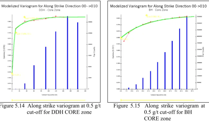
Table 5.5 Variogram modelization by zone for the DDH...44
Table 5.6 Variogram modelization by zone for the BH...44
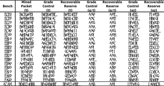
Table 6.1 Reserve by zone for mined packet - recoverable reserve - grade control model.56 Table 6.2 Reserve above 0.5 g/t by bench for mined packet – recoverable reserve - grade control model...57
Table 6.3 Cross validation statistics for DDH data set ...60
Table 6.4 Cross validation statistics for BH data set ...60
Table 6.5 Classification for DDH data...61
Table 6.6 Classification for BH data...61
Table 7.1 Estimated vs actual grade of gold mining project in Australia (Warren, M.J. 1991) ...66
Table 7.2 Parameters used for the Whittle 4X optimization...78
Table 7.3 Output of Whittle optimization for the pit shell 29...83
Table 7.4 Incremental pit shell characteristics based on pushback sequence 13-21-29 ...87
Table 7.5 Cumulative pit shell characteristics based on pushback sequence 13-21-29...87
Table 7.6 Whittle life of mine scheduling based on mining sequence #13, #21, #29 ...88
List of Figures
Figure 1.1 Flowchart: From exploration to mining...3
Figure 1.2 Location of Chibougamau ...7
Figure 1.3 Location of Troilus Mine...8
Figure 1.4 Mineralized boulder leading to the discovery of the 87 zone...9
Figure 2.1 Geology of Troilus - Plan view ...13
Figure 2.2 Geology of Troilus – Section 13600N...14
Figure 2.3 Gold mineralization of Troilus ...16
Figure 3.1 Diamond dill holes (DDH) selected ...20
Figure 3.2 Plan View 5360 - 0.2 g/t Au envelopes ...23
Figure 3.3 Section 13400N - 0.2 g/t Au envelopes...23
Figure 3.4 Plan View 5360 - New set of envelopes developed ...24
Figure 3.5 Section 13400N – New set of envelopes developed...24
Figure 3.6 Contact profile analysis of the new set of envelope developed based on DDH..26
Figure 4.1 1m assay for hole KN-88...30
Figure 4.2 3m composite for hole KN 88 ...30
Figure 4.3 DDH 3m assay composites historgram for ALL zone ...32
Figure 4.4 BH assay histogram for ALL zone ...32
Figure 4.5 DDH 3m assay composites histogram for HW zone...32
Figure 4.6 BH assay histogram for HW zone ...32
Figure 4.7 DDH 3m assay composites histogram for CORE zone...33
Figure 4.8 BH assay histogram for CORE zone ...33
Figure 4.9 DDH 3m assay composites histogram for FW zone...33
Figure 4.10 BH assay histogram for FW zone...33
Figure 4.11 DDH 3m assay composites histogram for 87S zone ...33
Figure 4.12 BH assay histogram for 87S zone...33
Figure 5.1 Grade Contour Map – Bench 5290...36
Figure 5.2 Parameters used in the calculation of the variogram...37
Figure 5.3 Cumulative distribution function of DDH assay for ALL zone ...39
Figure 5.4 Cumulative distribution function of BH assay for ALL zone ...39
Figure 5.5 Cumulative distribution function of DDH assay for HW zone ...40
Figure 5.6 Cumulative distribution function of BH assay for HW zone ...40
Figure 5.7 Cumulative distribution function of DDH assay for CORE zone ...40
Figure 5.8 Cumulative distribution function of BH assay for CORE zone ...40
Figure 5.9 Cumulative distribution function of DDH assay for FW zone...41
Figure 5.10 Cumulative distribution function of BH assay for FW zone ...41
Figure 5.11 Cumulative distribution function of DDH assay for 87S zone...41
Figure 5.12 Cumulative distribution function of BH assay for 87S zone...41
Figure 5.13 Parameters of a variogram...43
Figure 5.14 Along strike variogram at 0.5 g/t cut-off for DDH Core zone ...45
Figure 5.15 Along strike variogram at 0.5 g/t cut-off for BH Core zone ...41
Figure 5.16 Across strike variogram at 0.5 g/t cut-off for DDH CORE zone ...46
Figure 5.17 Across strike variogram at 0.5 g/t cut-off for BH CORE zone ...46
Figure 5.18 Downhole variogram at 0.5 g/t cut-off for DDH CORE zone...46
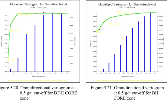
Figure 5.20 Omnidirectional variogram at 0.5 g/t cut-off for DDH CORE zone ...47
Figure 5.21 Omnidirectional variogram at 0.5 g/t cut-off for BH CORE zone ...47
Figure 6.1 Calculation of the estimated grade based on indicator kriging ...51
Figure 6.2 Bench 5290 - Mined packet...54
Figure 6.3 Bench 5290 – Recoverable reserve ...54
Figure 6.4 Bench 5290 – Grade control...54
Figure 6.5 Cross validation of the HW zone for the DDH data...62
Figure 6.5 Cross validation of the HW zone for the DDH data...62
Figure 6.6 Cross validation of the CORE zone for the DDH data...62
Figure 6.7 Cross validation of the FW zone for the DDH data ...63
Figure 6.8 Cross validation of the 87S zone for the DDH data ...63
Figure 7.1 Difference between kriging and simulation...68
Figure 7.2 Example of the determination of a node grade...71
Figure 7.3 Section 13400N – Recoverable Reserve Model ...72
Figure 7.4 Section 13400N – Simulation #5...72
Figure 7.5 Section 13400N – Simulation #11...72
Figure 7.6 Section 13400N – Simulation #18...72
Figure 7.7 Bench 5290 – Recoverable Reserve Model...73
Figure 7.8 Bench 5290 – Simulation #5 ...73
Figure 7.9 Bench 5290 – Simulation #11 ...73
Figure 7.10 Bench 5290 – Simulation #18 ...73
Figure 7.11 DDH 3m assay composites histogram for HW zone...75
Figure 7.12 Simulation #18 histogram for HW zone...75
Figure 7.13 DDH 3m assay composites histogram for CORE zone...75
Figure 7.14 Simulation #18 histogram for CORE zone...75
Figure 7.15 DDH 3m assay composites histogram for FW zone...75
Figure 7.16 Simulation #18 histogram for FW zone ...75
Figure 7.17 DDH 3m assay composites histogram for 87S zone ...76
Figure 7.18 Simulation #18 histogram for 87S zone ...76
Figure 7.19 Q-Q plot between DDH and simulation #18 for the HW zone ...76
Figure 7.20 Q-Q plot between DDH and simulation #18 for the CORE zone ...76
Figure 7.21 Q-Q plot between DDH and simulation #18 for the FW zone ...77
Figure 7.22 Q-Q plot between DDH and simulation #18 for the 87S zone...77
Figure 7.23 Exported Pit Shell for Pit #29 (340$US/oz) ...79
Figure 7.24 Ultimate pit design as of July 2001 ...79
Figure 7.25 Discounted open pit value for best case mining schedule ...81
Figure 7.26 Discounted open pit value for worst case mining schedule...81
Figure 7.27 Standardized probability distribution of discounted open pit value for best case ...84
Figure 7.28 Standardized probability distribution of discounted open pit value forworst case...84
Figure 7.29 Standardized probability distribution of Au produced ...85
Figure 7.30 Whittle pit by pit graph for Recoverable Reserve model ...86
Figure 7.31 Possible mill feed tonnage...90
Chapter 1
Introduction
1.1 General
introduction
With most commodity prices near all time low in the last several years and exploration expenditures kept to a minimum, mining companies had to rely on breakthroughs in technology to lower their operating costs and find new deposits. Amongst new technology developed, we can mention the global positioning system (GPS), the haul truck dispatch system, the drill navigation system, heap leaching, bio-leaching and a series of geophysical methods such as induced polarisation (IP), magnetic resistivity and so on. Also included in this group are techniques used to model and estimate mineral deposits. Recently developed techniques comprise indicator-based algorithms for kriging and conditional simulation. During the last 20 years, mining companies realized that in order to stay competitive and maintain their profit margin, they not only had to embrace those new technologies, but also to invest in research and development. People at Inmet Mining, understood this and decided to fund the present project. The objective of this project was to estimate mineral reserves of the Troilus gold deposit with a non-linear interpolation method and to assess the uncertainty of the mineralization through conditional simulation.
The first chapter presents a general introduction of the project. History and description of geostatistics and the Troilus mine are presented. The second chapter describes the geological context in which the Troilus deposit has been created. The third chapter gives details about how the assay data have been used to develop a geological interpretation of the grade distribution. The fourth chapter deals with the compositing of the diamond drill holes and the blasthole data set. Analysis of the spatial continuity is the subject of chapter five. Reserve estimation and the selection of the interpolation method are discussed in chapter six. Chapter seven treats conditional simulation and the different approach used to analyse the risk. Finally, chapter eight summarizes the results and gives some recommendations for future work.
1.2 Description
of
geostatistics
1.2.1 Introduction
Because mining investments are generally large, the economic consequences of making investment decisions are very important. Therefore, it is crucial that we evaluate the global and local resources very carefully (Clark, I and Frempong, P.K. 1996). The science used for this is called geostatistics. Geostatistics is the use of classical statistical methods adapted to the mining and geological context. Geostatistics distinguish itself from the classical statistical method by the use of spatial information of the variable under study. Examples of such variables are:
ore grades in a mineral deposit
depth and thickness of a geological layer porosity and thickness of a geological unit density of trees of a certain species in a forest soil properties in a region
pressure, temperature and wind velocity in the atmosphere concentration of pollutants in a contaminated site
In addition to that, the science of geostatistics is based on regionalized variables and not on random variables. The grade of a gold sample cannot be categorized as a random variable, since its constitution (grade, location) has been influenced by its position and its relationship with its neighbours. Consequently, the general objectives of geostatistics are to characterize and interpret the behaviour of the existing sample data and to use that interpretation to predict likely values at locations that have not been sampled yet.
1.2.2 Geostatistics and mining
In the mining industry, people usually refer to the word geostatistics to describe the amalgamation of the diverse estimation studies realized between the completion of the drilling campaign and the design of the excavation. In most cases, geostatistics is used to
quantify a mineral resource. Estimates of the tonnage and grade are first carried out to give the company and the investor community an idea of the resource potential.
Figure 1.1 Flowchart: From exploration to mining
This estimate is then subdivided into classes based on the level of confidence. Mineral reserve estimates require the contribution of different people with different sets of skills. The flowchart of figure 1.1 shows the different components involved in the development of a mineral reserve base. First, preliminary exploration works such as geology mapping, soil sediment analysis, geochemistry and geophysics are carried out to understand and assess the geological potential of the exploration property. Depending on the results, a drilling campaign could be launched for the purpose of finding enough mineralization of interest to carry the project forward. Up to this stage, exploration geologists are usually in charge of the project. Their focus is mainly to relate the mineralization with geological features such as alteration, lithology and structure. They are also in charge of the geological interpretation of the orebody and its subdivision into different zones. The geostatistician involvement in the project begins when information collected from the exploration campaign results in
Geological Interpretation Domain Development DDH Compositing Variography Univariates Statistics Cross Validation Resource Classification Interpolation Resource
Optimization Pit Design Economics
Parameters
Scheduling Cash Flow Reserve
enough data to allow a resource estimate concerning the size and potential of the project. Geostatistical analysis of the deposit will provide valuable information, for instance:
mean, variance and other statistical parameters through univariates statistics a measure of continuity of the mineralization through variography
possible tonnage and grade of the deposit through interpolation method
From this information, a resource estimate will be generated by the geostatistician. This will represent the overall potentially valuable material that is contained within the deposit. Based on the level of geological knowledge and confidence, this resource estimate will be divided into inferred, indicated and measured categories (Anderson, M.J. 1999). Armed with this resource estimate, the exploration geologist will try to add material into each category with more drilling and by proving geological and grade continuity. The mine planning engineer will start to get involved in the project when the measured and indicated resources have sufficient potential material to warrant a preliminary economic assessment. At this stage, the aim is to determine if the current resource has the potential to be mined. This will be evaluated by incorporating mining, processing, financial, environmental, social and legal factors into the resources. If the resources prove to be economical, material previously categorized as measured and indicated will be moved into the reserve categories of proven and probable. In some cases, measured resources will become probable reserves. They will be followed by more detailed work such as excavation design (open pit or underground), process design, environmental impact study and so on, which might ultimately lead to a decision to proceed with the development of a future mine.
1.2.3 History of geostatistics
The application of geostatistics to problems in geology and mining dates back to the early 40’s, when Herbert S. Sichel worked on some South African gold mines on the development of a method to predict the grade of an area to be mined from sparsely gold samples. Sichel’s work involved the creation of a lognormal distribution table that enabled the calculation of the average of a lognormal variable such as gold. In the 50’s, Daniel G. Krige collected an exhaustive set of gold assay data from South African mines. Following that, Krige developed a technique called "Weighted Moving Average" which is a linear
regression used to estimate the value of mining blocks. In 1960 in Sweden, Bertil Matern applied the concept of spatial statistics of forestry industry data.
Among those who have contributed to advance the science of geostatistics, George Matheron is surely the one who moved the geostatistical science to the level known today. During the 1954-1963 period, Matheron rediscovered the pioneering work carried out on the gold deposit of the Witwatersrand by Sichel, Krige and de Wijs, and built the major concepts of the theory for estimating resources, which he named Geostatistics. Between 1962 and 1965, Matheron published two books: "Treatise of Applied Geostatistics" (1963) and "The Regionalized Variables and their Estimation" (1965). The former lays down the fundamental tools of linear geostatistics: variography, variances of estimation and kriging. The latter is his PhD thesis and explains in a more theoretical way the concept of geostatistics. In 1968, the Paris School of Mines created the "Centre de Géostatistique et Morphologie Mathématique" of which Matheron became the director. From 1968 to his retirement in 1996, collaborators such as André Journel, Alain Maréchal and Pierre Delfinerl helped to create the concept of non-linear and non-stationary geostatistics. The period 1980-2000 will see the creation of geostatistical methods for specific applications. The non-parametric geostatistics was developed during the 80’s by André Journel to counteract the smearing effect of ordinary kriging on erratic mineralization. With the technological revolution of the 80’s, computers became available to a broader range of people, making geostatistics more accessible. Today, conditional simulation algorithms are used in the mining industry to assess the variability of the mineralization and to analyse the sensitivity of ore reserve estimation. The science of geostatistics is not only used in mining, but in a broader range of industries such as: petroleum, forestry, agronomy, oceanography, meteorology, fishery, environmental science, etc…
1.3 Computer
software
Due to the large amount of data treated and the numerous geostatistical interpolations and iterations required for the project, the utilization of a powerful pc and the most advanced geostatistical software were a necessity. The principal software used was Gemcom. It is a general mining package capable of treating information coming from geological exploration
up to the design of an open pit mine. In this case, Gemcom was specifically used for geological modelling, compositing and reserve estimation. The analysis of the spatial continuity was carried out with Supervisor, a geological software provided free of charge by Snowden Mining Industry Consultants Pty Ltd of Australia. Supervisor is the grouping of two different softwares: Analysor and Visor. Snowden Analysor was used to generate the univariates statistics for the DDH and BH data and Snowden Visor was used to generate the multiple variograms for the DDH and BH. The conditional simulations were carried out with WinGSLIB, the Windows version of GSLIB. And finally, conditionally simulated models were assessed through a series of pit optimization algorithms using Whittle 4X.
1.4 Troilus
Mine
1.4.1 Location
The town of Chibougamau is located 510 kilometres north of Québec, Canada (figure 1.2). The Chibougamau area has been a major gold camp during the 1960’ and 1970’.
Figure 1.2 Location of Chibougamau
Today, however, only three mines are in operation: Joe Mann and Copper Rand, both underground mines owned and operated by Campbell Resources and Troilus, an open pit mine owned and operated by Inmet Mining. The Troilus Mine is located 174 kilometres north of Chibougamau (figure 1.3). It is accessible by the "Route du Nord" up to 44 kilometres from the site, where a gravel road accesses the property.
Figure 1.3 Location of Troilus Mine
1.4.2 Historic of Troilus
In 1958, after the discovery of mineralized boulders in the region of the Frotet Lake and Troilus Lake, initial exploration work began. Between 1958 and 1967, some copper and zinc anomalies were identified, including the Baie Moléon massive sulphide deposit discovered in 1961 by Falcondbridge Limited. This small deposit contains mineral resources of 200 000 tonnes at 2.0% Cu, 4.25% Zn, 39.7 g/t Ag and 1.0 g/t Au. In 1971, the Lessard deposit (1.46 Mt at 1.73% Cu, 2.96% Zn, 38.0 g/t Ag and 0.70 g/t Au) was discovered around the Domerque Lake by Selco Mining Corporation. Following this discovery, a geophysical survey of the Frotet Lake and Troilus Lake area was carried out, unfortunately without significant results.
In 1983, the Quebec government released the results of a new geophysical survey. Following the release, some groundwork was carried out again without any major results. In 1985, the Ministry of Energy and Natural Resource of Quebec published a study from a field mapping survey, which indicated some potential for the region to host gold and base metal deposits. Kerr Addison Inc immediately staked an important group of claims in the
area and kicked off an exploration program consisting of field mapping, geophysical survey, geochemistry and core drilling. Finally, the 87 zone was discovered in 1987 following the recovery of a mineralized boulder (figure 1.4).
Figure 1.4 Mineralized boulder leading to the discovery of the 87 zone
In October 1988, a joint venture agreement between Kerr Addison Inc and Minnova Inc was reached. During 1991, a 50-man capacity exploration camp was built between the 87 and J4 zone. During that year, exploration drilling was carried out and a 200 tonnes bulk sample averaging 2.3 g/t Au was taken from the middle of the 87 zone. Of the 200 tonnes bulk sample, 100 tonnes was processed in the facilities of the Centre de Recherches minérales du Québec for a pre-feasibility study; and in 1993, the remaining 100 tonnes were processed at Lakefield pilot plant for a feasibility study. Between December 1992 and March 1993, infill drilling was completed to improve the definition of the 87 and J4 zones and to test some anomalies from the latest geophysical survey. Over the period 1988 to 1993, 565 DDH holes were drilled from surface for a total of 84,600 meters. In February 1993, Metall Mining Corporation took control of Minnova Inc from Kerr Addison Inc and in May 1993, Metall Mining Corporation bought out Kerr Addison’s interest in the property. In September 1993, after a due diligence by Coopers and Lybrand of Toronto, the feasibility concluded in the viability of the project. In 1994, Metallgesellscaft AG from Germany sold is 50.1% part in Metall Mining Corporation. Shortly after, Metall Mining Corporation changed its name for Inmet Mining Corporation, which come from the words International and Metals. Finally, in June 1995, financing of the project was completed with a consortium of international banks.
Construction of the Troilus mine began at the end of 1994 and was completed during 1996. The mine being located on land owned by a Cris native band, Inmet agreed to locally employ at least 25% of the mine workforce. Initially, the project had a price tag of 160 million $CDN, but due to problems related to supplies, construction management and a change in the mine plan during the construction phase, the final price came in at 200 million $CDN. The original ore reserve of the Troilus deposit, based on a gold price of 375$US were 49.6Mt at a grade of 1.4 g/t. The mine started commercial production in October 1996 and has run continuously since.
1.5 Problematic
and
objectives
Many resource/reserve estimates have been carried out on the Troilus deposit over the years. In the majority of the cases, the estimates have been produced by people with limited amount of knowledge and familiarity with the orebody. Although not in their mandate, most of them did not have the chance to question or challenge the underlying hypothesis on which their estimates were based. Moreover, due to time constraints and budget limitations, none of them had the opportunity to take into consideration the effect of local and global uncertainty on their estimates. In view of that, the overall objective of this project is to reconsider the assumptions on which previous resource estimates were based and to assess the significance of uncertainty on the estimates.
First, this thesis will investigate a different approach to the geological interpretation of the Troilus orebody. The modelling of geological features imperative to the grade interpolation is one of the most important steps of a resource/reserve estimate. This phase of the project will serve as the basis from which compositing, variography and interpolation will be derived from. Erroneous or misguided geological interpretation can artificially inflate the ore tonnage of a zone or can include more waste material than it should be.
Secondly, the effect of uncertainty on local estimates will be explored. Instead of only using the distance to assign the grade of a block, this project will include another component that will improve the local estimates. This element is the local distribution of the gold assay surrounding the block to be estimated and it will be incorporated during the interpolation process.
Finally, global uncertainty of the estimates will be assessed through conditional simulation. Through the generation of multiple equi-probable scenarios of mineralization, an analysis of the risk inherent to the orebody will be realized.
CHAPTER 2
Geology
2.1 Introduction
The presentation that follows of the geology of the Troilus deposit was mostly based on an internal report written by Inmet exploration geologist Bernard Boily entitled " Porphyry-type mineralization in the Frotet-Evans greenstone belt – The Troilus Au-Cu deposit". First, the regional and local geology contiguous of the Troilus deposit will be described. Thereafter, characteristics pertaining to the Troilus deposit, such as alteration, mineralization, structure, foliation and in-situ density will be presented.
2.2 Regional and local geology
The Troilus deposit lies within the Frotet-Evans Archean greenstone belt. The greenstones consist of submarine mafic volcanics and cogenetic mafic intrusions. Felsic volcanics and pyroclastic rocks are also present along with epiclastic sedimentary units and ultramafic horizons (figure 2.1, 2.2). Late granitoid plutons and dykes intrude the greenstones. The intrusive rocks range from pre to post tectonic in age. Regional deformation has taken place and produced strong regional foliation. Sub-horizontal mega to mesoscopic folding has affected both the primary layering and regional foliation. Metamorphic grade in the Troilus area ranges from greenschist to lower amphibolite facies. The higher grade metamorphism occurs around the borders of certain intrusions and towards the margins of the greenstone belt. The Frotet-Evans belt is known for its numerous volcanogenic massive sulphide (VMS)deposits. Troilus is the only disseminated Au-Cu volcanic porphyry type deposit located in the belt so far.
2.3 Troilus
deposit
2.3.1 Geology and alteration
Two main zones, 87 and J4 have been outlined as well as two sub-economic zones, 86 and J5. The 87 and J4 zones are presently being mined and the amount of information on those zones are much greater than the others. The 87 and J4 zones are hosted in an intermediate porphyritic volcanic unit within which are found elongated zones of hydrothermal breccia and coeval feldspar quartz porphyry dyke/sill swarms (figure 2.1).
Figure 2.1 Geology of Troilus - Plan view
These rocks dip moderately (60-70) to the northwest (figure 2.2). The 87 zone has a wide continuous core of ore (up to 100 m) over some 300 m of strike length. The north and south continuations are bifractated and form narrowing branches of ore amongst weakly mineralized rock.
Figure 2.2 Geology of Troilus – Section 13600N
Two branches are well defined in the north. Three branches are less well displayed to the south. The mineralization seems to rake moderately to the north at about 35. The J4 zone appears to consist of pipe shaped zones. Continuity between sections is not as well established as in the 87 zone. The central part of the mineralized zone coincides with an in situ hydrothermal breccia, which exhibits pseudo-fragments of porphyritic intermediate volcanic rocks in a strongly foliated and altered (biotite-amphibole) matrix. The brecciated texture of the rock comes from the development of polygonal fracturing which channeled hydrothermal solutions. The white colored albitized pseudo-fragments in the breccia represent the less altered portion of the rock.
The breccia is transected by porphyritic felsic dyke swarms, a few mafic dykes and by several deformed small chalcopyrite-bearing quartz veins. Polygonal fractures are abundant in the felsic dykes and are interpreted to have formed during the cooling process of the dykes (columnar jointing). These fractures are also mineralized and Au-bearing thus suggesting that the dykes and the mineralization are contemporaneous. One of the felsic dykes has yielded a radiometric age of 2,786 Ma 6 Ma, based on U-Pb dating of zircon.
All these observations suggest that the formation of the Troilus orebody is pre-metamorphic. The main alteration facies defined during the course of core-logging and geological observations made in the pit include, from earliest to latest:
1. Hornfels (very fine biotite)
2. Potassic (biotite – actinolite – K-feldspar) 3. Inner Propylitic (actinolite - albite - epidote) 4. Outer Propylitic (albite - epidote - calcite) 5. Phyllic (sericite - quartz)
The formation of the hydrothermal breccias and the intrusion of the dyke swarms are contemporaneous. Both are deformed and it is interpreted that the effects of tectonism must have ceased during the formation of the potassic assemblage. Potassic, propylitic and phyllic alteration facies are spatially associated with ore. The geological nature of the orebody does not significantly impact the operation. Perhaps the main influence noted to date is that the dykes fragment and comminute differently than the breccia and other volcanic rocks. To what degree these breakage functions affect the operation is not known. Another factor that has no impact but does provide some visual indication of better zones is the amount of biotite. Zones with more biotite correspond closely with better grades.
2.3.2 Mineralization
Chalcopyrite and pyrhotite, with subordinate pyrite, are the main sulphides encountered in the central part of the deposit. The sulphides are most abundant in the breccia matrix along with biotite enrichment. The breccia fragments or protoliths are less enriched. In general, it is thought that the original metalliferous fluids percolated through the rock along openings around the fragments of the volcanic breccia. Ongoing alteration and metamorphic re-mobilization caused further digestion of the protoliths and infiltration of metal rich fluids into the fragments. Hence in the more altered core of the deposit, the fragments are less evident (almost entirely altered) and metal enrichment is ubiquitous. Towards the margins, the fragments are better preserved and metals are restricted more within the matrix infilling.
Hence the mineralization can be characterized as essentially "disseminated" in the core and stringer or sheared towards the margins (figure 2.3).
Figure 2.3 Gold mineralization of Troilus
The felsic dykes intruding the breccia contains almost exclusively pyrite. They usually form ore but are poor in copper. There appears to have been at least two phases of mineralization. The first was copper rich and the second gold rich. The two do not exactly overlay. The copper envelope is offset towards the east with respect to the gold envelope. A typical cross section from west to east would have a gold rich, copper poor, hanging wall partition; a wide gold rich and copper rich mid region; and a copper rich gold poor footwall region. Within the central part (more or less the center of the copper envelope) there is a 15 m wide zone of strong copper enrichment (>0.2% Cu). The copper envelope bulges to the east in the north regions and there are some additional copper rich lenses further into the footwall (outside of the pit walls).
About 25% of the gold reports to dore bars through a gravimetric circuit. The origin of this free gold mineralization has not been accurately located. However if it follows regions of erratic high grade assays, then it would be found closer to the less altered margins and within narrower stringer zones particularly towards the north.
The nature of the mineralization has important implications on the methods used in sampling (lengths of cores, blasthole sampling tools), assaying (size of fire assay, metallic screening) and in interpolating grades within the block model (continuity, top cutting, variogram nugget effect). Also the mineralization affects the mill circuit and recoveries (copper flotation particularly). Although the knowledge of the mineralization has increased, no clear procedures have been established to deal with the differences in mineralogy since the various zones are not easy to localize (not large or discrete enough) and in any case, the selectivity of the mining equipment and short ore supply precludes the use of detailed selection and blending of ore zones to the degree necessary to follow the changes in mineralization. Outwards from this copper/gold-rich zone, chalcopyrite becomes subordinate and pyrite, with lesser pyrhotite, predominates and is particularly abundant over the northern portion of the 87 Zone. This zone overlaps the transition between the potassic and the inner propylitic alteration facies. This area is often characterized by sodic, rather than potassic, alteration.
2.3.3 Structure and foliation
Three main fracture orientations were observed. The first set, oriented at 215 (true north) and dipping at 63, is sub-parallel to the regional foliation and represents the major fracture system in the pit area. The other two sets (035/39 and 320/85) cut the regional foliation almost at right angles. The combined effect of these fractures has induced local instability in the pit and is directly responsible for the blocky nature of the walls. Faulting is observed in several areas of the pit. A normal dexter fault (315/55 dip NE mine grid) cuts through and changes the orientation of the mineralization. A second fault in the SE pit region (220/40 NW) is associated with chalcopyrite enrichment. Regional deformation has strongly flattened and stretched the geological assemblages and alteration pattern.
In the pit area, the effects of this deformation can be observed as follows: strongly elongated felsic dykes (all parallel to the regional foliation); and stretching of the hydrothermal breccia.
2.3.4 In-situ density
The bulk density of in-situ rock is taken as 2.77 t/m3. For broken muck and stockpiled material, 1.90 t/m3 is used while overburden weight is 2.20 t/m3. The value for rock was derived from measurements on drill cores samples and in-pit samples.
2.4 Conclusion
The Troilus deposit lies within the Frotet-Evans Archean greenstone belt. It is the only disseminated Au-Cu volcanic porphyry type deposit located in the belt so far. The deposit consist of two zones, 87 and J4. These zones are hosted in an intermediate porphyritic volcanic unit within which are found elongated zones of hydrothermal breccia. The mineralization can be characterized as disseminated in the core and stringer or sheared towards the margins. There appears to have been at least two phases of mineralization. The first was copper rich and the second gold rich. The mineralization has an azimuth of 35° and dip 60° to 70° to the northwest. Approximately 25% of the gold is free and is recovered by a gravimetric circuit.
CHAPTER 3
Geological Modelling
3.1 Introduction
The geological modelling of an ore deposit entails the separation of mineralization population into homogeneous groups (Coombes, J. 1997). This is done by grouping the mineralization according to geological features such as alteration, foliation, structural unit, and grade homogeneity. At Troilus, the nature of its volcanic porphyry type deposit and its simple geometric configuration makes it somewhat less of a challenge on the modelling side. However, the disseminated feature of the deposit means that more time will have to be spent on modelling the "high grade" core of the deposit to limit its influence on lower grade area. First, a review of the data (DDH, BH) on which the modelling will be based will be carried out to ensure its integrity. Modeling of the grade distribution into subset of homogeneous population will then take place. Finally, assessment of the modelling through a contact profile analysis will be done to confirm the validity of the modelling.
3.2 Database
3.2.1 Diamond drill hole (DDH)
The diamond drill hole (DDH) database on which the recoverable reserve block model and the conditional simulation were based contains information of the exploration and definition drilling campaigns from 1988 to 1999. The database contains a total of 625 holes covering the 87 zone, 87S zone, J4 zone and other exploration targets. Drilling was carried out on parallel fence lines spaced nominally 25 m apart for the upper 25% of the deposit and on every second section (50 m apart) for the deeper holes. Of those 625 holes, only 314 were used for the current grade interpolation. The selected holes cover the area of the 87 and 87S zones (figure 3.1). The database contains assay results for gold in grams per tonne (Au g/t), silver in grams per tonne (Ag g/t) and percent (Cu %). For the purpose of the current study, only gold assay were used for the grade interpolation. This can be related to
the fact that at Troilus, 85% of their revenue is derived from gold and also that main ore reserve problem associated with grade interpolation is related to the gold mineralization.
Figure 3.1 Diamond dill holes (DDH) selected
3.2.2 Blasthole (BH)
The blasthole (BH) database used to create the grade control block model contains data from all the blastholes drilled from the beginning of the operation in 1996 until the end of February 2002. The database contains a total of 171,396 blastholes covering the 87 and 87S zones. The average distance between holes, based on the production drilling pattern, which is 5.1 metres by 5.9 meters. The database contains assays for gold in grams per tonne (Au g/t), copper in percent (Cu %) and the NSR (net smelter revenue) value in Canadian dollar per metric tonne (NSR $CAN/t). Again, only gold assay were used for the grade interpolation.
3.2.3 Review
A thorough verification of the DDH and BH database has also been conducted to make sure that the data used for grade interpolation do not contain any data entry errors and that no
data are missing. Since many people have used the current databases, either the mine personnel or external consultants, most of the errors have been sorted out.
3.3 Geological
interpretation
3.3.1 Definition
The geological interpretation of an orebody is the most crucial step in resource/reserve estimation. It involves the analysis and interpretation of the following elements:
type of deposit (porphyry, massive sulphide)
types of mineralization in the deposit (laterite, oxide, sulphide) continuity of mineralization (metres, kilometres)
structural element of the deposit (fault, vein, dyke) spatial distribution of the grade (Au, Cu, Zn)
Most of the time, the geological interpretation used is a computerized simplification of a system far more complex in nature. This comes from the fact that it is almost impossible to model every aspect of a deposit. Despite the fact that we end up with a geological interpretation that is quite simple compared to reality, it is accurate enough for the purpose of grade interpolation. The main reason of creating geological domains or envelopes is to separate data into populations. By combining data that are deemed homogeneous over a domain, the stationary concept can usually be adopted (Goovaerts, P. 1997). Conversely, the availability of enough data to the infer semi-variograms as well as the ability to differentiate different populations will render the subdivision of the data into different domains feasible or not. If possible, it will have a positive effect on kriging by reducing the nugget effect (variability) and by increasing the range of mineralization (continuity).
3.3.2 Problematic and avenue
Previous resource/reserve estimates at Troilus were realized on a set of envelopes based on a cut-off grade of 0.2 g/t Au (Geostat Systems International Inc. 1995). The corresponding set of envelopes was developed on the idea that the mineralization seems to transcend most
lithologic contacts, alteration assemblages and structural domain (Sim, R. 1998). This assumption leads toward the use of "soft" boundaries, which may be diffuse or gradational and result in an over-smoothing of the estimates. In fact, only 2 sets of envelopes had a real impact on the outcome of the grade interpolation; the envelope "Zone #1" for the 87 zone and the envelope "Zone #4" for the 87S zone (figure 3.2, 3.3). Since the current set of envelopes has no boundaries between the high grade and low grade material, the Troilus engineering/geology group reported problems related to the smearing of the grade estimates. One possible avenue to overcome this problem was to change the way the envelopes have been developed. This had previously been carried out by Geostat and the geology group of Troilus (Geostat Systems International Inc. April 1997). By looking at a typical section of the 87/87S zone (figure 3.5), intuitively it can be seen that a core of high grade material exists for both zones. The newly set of envelopes developed are only based on the spatial distribution of the 3m composited gold grade. This comes from the fact that no correlation has been measured so far between the gold distribution and any geological features such as rock type, structure or alteration. In this situation, it is still better to use some sort of local control over the mineralization with an envelope based on grade (Blackney, P.C.J. and Glacken, I.M. 1998). Based on those facts, the "zone #1" has been split into 3 different zone named HW (hangingwall), FW (footwall) and CORE. For the "zone #4", it has been tightened up and renamed 87S (figure 3.4, 3.5). Instead of having one set of variograms for 3 different grade domains as before, the new set of envelopes will have 3 sets of variograms. This should increase the range of continuity of the main zone (CORE) and reduce it for the transitional low grade envelope (HW, FW). The smearing, which took place with the old set of envelopes, should therefore be reduced.
Figure 3.2 Plan View 5360 - 0.2 g/t Au envelopes
Figure 3.4 Plan View 5360 - New set of envelopes developed
3.4 Contact profile analysis
3.4.1 Definition
A useful tool to evaluate the validity of an envelope is the use of a contact profile analysis. A series of average grades are calculated for different distances inside an envelope and a graph is produced showing the grade change from an envelope to another. If there is a distinct difference in the average grades across a boundary, then there is evidence that the boundary may be important in constraining the grade estimation. On the other hand, if a "hard" boundary is imposed where grades tend to change gradually, grade may be overestimated on one side of the boundary and underestimated on the other side.
3.4.2 Application
Contact profile analysis has been carried out on the new set of envelopes developed for the DDH data between the HW-CORE zone, CORE-FW zone and FW-87S zone. It can be clearly seen from the following graphics (figure 3.6) that a net difference exits between the low grade envelope (HW, FW) and the high grade envelope (CORE, 87S). The HW envelope has an average of 0.31 g/t Au over the 45 meters analysed compared to 1.08 g/t Au for the CORE zone. For the CORE-FW profile, the CORE envelope has an average of 1.08 g/t Au and the FW zone has an average of 0.35 g/t Au. The same trend exists between the FW (0.23 g/t Au) and the 87S zone (0.98 g/t Au).
Figure 3.6 Contact profile analysis of the new set of envelope developed based on the DDH
Contact Profile Between HW Zone and CORE Zone
0.0 0.2 0.4 0.6 0.8 1.0 1.2 1.4 1.6 1.8 -4 7. 5 -4 2. 5 -3 7. 5 -3 2. 5 -2 7. 5 -2 2. 5 -1 7. 5 -1 2. 5 -7 .5 -2 .5 2.5 7.5 12 .5 17 .5 22 .5 27 .5 32 .5 37 .5 42 .5 47 .5
Distance from Contact (m)
Au ( g /t ) HW Zone CORE Zone
Contact Profile Between CORE Zone and FW Zone
0.0 0.2 0.4 0.6 0.8 1.0 1.2 1.4 1.6 1.8 -4 7. 5 -4 2. 5 -3 7. 5 -3 2. 5 -2 7. 5 -2 2. 5 -1 7. 5 -1 2. 5 -7 .5 -2 .5 2.5 7.5 12 .5 17 .5 22 .5 27 .5 32 .5 37 .5 42 .5 47 .5
Distance from Contact (m)
Au ( g/ t) CORE Zone FW Zone
Contact Profile Between FW Zone and 87S Zone
0.0 0.2 0.4 0.6 0.8 1.0 1.2 1.4 1.6 1.8 -47. 5 -42. 5 -37. 5 -32. 5 -27. 5 -22. 5 -17. 5 -12. 5 -7 .5 -2 .5 2.5 7.5 12. 5 17. 5 22. 5 27. 5 32. 5 37. 5 42. 5 47. 5
Distance from Contact (m)
Au ( g/ t) FW Zone 87S Zone
3.5 Conclusion
Modelling of the Troilus deposit has been greatly lightened by the nature of the orebody. In addition, in light of new information and actual mining experience, the original geological interpretation has been reviewed and updated. As a result, focus has been put not so much on associating gold grade to geological features such as alteration and structure but more on domaining the different grade population to minimize the smearing of high grade into the low grade area. Homogeneity of gold grade in each geological envelop has been obtain by subdiving the original Zone#1 and Zone #4 into four new zones named HW, CORE, FW and 87S. A contact profile analysis has been done on the new set of geological envelope and confirmed the merit of tighter envelope in order to achieve stationarity.
CHAPTER 4
Compositing
4.1 Introduction
The compositing of assay interval, also know as regularization, involved the grouping of assay of different interval into a standard length. Composites are in fact a 3D points with its centroid at the middle of the composite interval. Compositing has the benefit to standardize the weight attributed to each assay and to adjust the variability of the composites to be consistent with the scale at which the deposit will be mine. It has also the benefit of lowering the overall variability, which in turns help in modeling the experimental variograms. In the case of Troilus, composites are calculated within each geological envelope.
4.2 Diamond drill holes (DDH)
4.2.1 Sample data and composite statistics
The 314 holes of interest from the DDH database contain a total of 30,060 gold assays. These samples were composited into 3 metres down-the-hole intervals starting from the collar. This composite distance was chosen after taking into account the overall dip of the orebody. With a composite interval of 3 metres and an orebody dip of 60, this gives a vertical distance of approximately 2.5 metres between each sample. Tables 4.1 and 4.2 give statistics for the 1m assays and 3m composites for each zone.
Table 4.1 DDH 1m assay statistics
Zone samplesNumber Maximum Minimum Mean Median deviationStandard Variance Coefficient variation samples > 0.5Number Mean > 0.5
ALL 30,060 108.15 0.00 0.62 0.19 2.15 4.63 3.50 8,314 1.85
HW 9,182 42.99 0.00 0.27 0.10 0.84 0.71 3.14 1,160 1.30
CORE 7,767 103.01 0.00 1.22 0.62 2.76 7.63 2.26 4,413 1.98
FW 8,923 108.15 0.00 0.41 0.12 2.02 4.08 4.88 1,509 1.83
Table 4.2 DDH 3m composite statistics
4.2.2 Compositing variance
When compositing, the mean of the composited data should always be equal to the mean of the assay sample. No matter what the length of the composites we decide to use, the mean has always to be the same. In the present case, when the mean of the 1m assay sample is compared to the mean of the 3m down-the-hole composite samples, it can be see that the mean grade from the 3m composites data is lower. This aberration comes from the way the composites are calculated. In Gemcom, a down-the-hole composite is calculated from the collar of the hole. For example, if there is no 1m assay sample to calculate a composite, a grade of 0 g/t is going to be assigned to this composite. This has the effect of lowering the average grade of the composite sample. On figure 4.1 below, drill hole KN-88 has only one 1m assay sample for the first 48 meters of the hole. Once composited into 3m section, we can see that 15 composites have been added at a grade of 0 g/t (figure 4.2).
When the 87S zone is examined, we can find that the mean for the 3m composites is actually higher than the mean of the assay sample. This can be explained by the fact that in the DDH database, some holes drilled on the 87S zone in 1999 have been sampled at 3 meter intervals. So in this case, the 1m assay sample statistics are in fact a mixed of 2 assay sample population: 1m assay samples and 3m assay samples. This results in a lower mean grade for the 1m assay statistics, since the 3m assays are only counted once instead of being counted 3 times. Looking at the mean grade of the 1m assay sample versus the 3m composite assay at a 0.5 g/t Au cut-off, it can be see that a dilution effect is introduced when the drill holes are composited. In this case, three 1m assays are combined to create one 3m composite. Since there is more lower grade assay than high grade, the result of the compositing is an increase in the tonnage and reduction in the grade at a given cut-off.
Zone samplesNumber Maximum Minimum Mean Median deviationStandard Variance Coefficient variation samples > 0.5Number Mean > 0.5
ALL 13,378 100.08 0.00 0.54 0.19 1.78 3.17 3.31 3,696 1.58
HW 4,740 31.05 0.00 0.21 0.07 0.64 0.41 3.07 494 1.09
CORE 3,221 40.81 0.00 1.09 0.73 1.63 2.65 1.49 2,002 1.63
FW 3,777 53.89 0.00 0.36 0.14 1.25 1.56 3.44 634 1.45
Figure 4.1 1m assay for hole KN-88 Figure 4.2 3m composite for hole KN-88
4.3.1 Sample data statistics
For the BH assay database, no composites have been calculated. Since most of the database contains samples taken every 5 metres and, only lately, that 10 metre sample intervals have been introduced.
Table 4.3 BH assay statistics
Zone samplesNumber Maximum Minimum Mean Median deviationStandard Variance Coefficient variation samples > 0.5Number Mean > 0.5
ALL 189,415 73.54 0.00 0.65 0.34 1.02 1.04 1.57 73,991 1.36
HW 69,163 73.54 0.00 0.34 0.19 0.61 0.37 1.79 13,039 1.07
CORE 65,828 63.02 0.00 1.13 0.80 1.29 1.66 1.15 45,392 1.51
FW 48,925 69.03 0.00 0.46 0.24 0.84 0.71 1.83 13,605 1.19
On a size of support point of view, having a sample every 5 meters is more than enough and to composite those assays to a smaller support size would not add any benefits to the grade interpolation. Furthermore, when 10 meter samples are used, it is in an area where the level of confidence of the mineralization is high and where one or two samples will not make a difference on the outcome of the average grade when assigning the material type (Ore/Waste) for this hole.
4.4 Data set comparison
When we weigh the BH assay statistics (table 4.3) against the DDH 1m assay (table 4.1) and 3m composites statistics (table 4.2), we can notice the mean of the BH assay is very close to the mean of the 1m assay of the DDH. But when the means above the 0.5 g/t cut-off are compared, the correlation is now better between the BH assay and the DDH 3m composites. This indicates that the portion of the BH assay below the 0.5 g/t cut-off is at a higher grade than the same portion for the DDH 3m composites. Therefore, we can expect a higher overall grade and slightly higher tonnage above the 0.5 g/t cut-off for the Grade Control block model.
4.5 Distribution analysis for the DDH 3m assay composites and
BH assay
The shape of the histograms for both data sets clearly shows that the gold samples follow a lognormal distribution (figure 4.3 to 4.12). The lognormality of the distribution has been confirmed by taking the logarithms of the data thus creating a a normal distribution (bell shaped curve). This is also an insight to log transform the original data in order to ease the modeling of the variograms. In this case, a possible transformation could be either logarithmic or indicator. In addition, the shapes of the distribution suggest a highly positively skew set of data. This is also indicated by the fact that the standard deviation is more than three times the mean value. (Clark, I and Harper, W.V. 2000). The shape of the two data sets can be compared by looking at their respective quantiles for each geological zone. Comparison between the DDH 3m composite/BH data for the quantiles of the CORE zone and 87S zone shows a good correlation. The quantiles 25%, 50%, 75% for the
DDH/BH of the CORE zone is 0.29/0.41, 0.73/0.80 and 1.37/1.43 respectively. For the 87S zone, the correlation is 0.14/0.17, 0.32/0.34, 0.67/0.67 for the quantiles 25%, 50% and 75% respectively. On the other hand, the HW and FW zones show a poor correlation between the two data sets. For the HW zone, the correlation is 0.01/0.08, 0.07/0.19, 0.23/0.40 and for the FW zone, the correlation is 0.04/0.10, 0.14/0.24, 0.36/0.55. This can somewhat be explained by the lower amount of information (information effect) from the DDH, where the number of samples is more than 10 times less than that of the BH.
Figure 4.3 DDH 3m assay composites Figure 4.4 BH assay histogram for ALL
histogram for ALL zone zone
Figure 4.5 DDH 3m assay composites Figure 4.6 BH assay histogram for HW
histogram for HW zone zone
Au Histogram DDH - HW Zone 0.00 0.05 0.10 0.15 0.20 0.25 0.30 0.35 0.40 0.45 0.50 0.55 0. 00 0. 10 0. 20 0. 30 0. 40 0. 50 0. 60 0. 70 0. 80 0. 90 1. 00 1. 10 1. 20 1. 30 1. 40 1. 50 1. 60 1. 70 1. 80 1. 90 Au (g/t) Fr e q u e ncy Points: 4,740 Mean: 0.208 Std Dev: 0.640 Variance: 0.409 COV: 3.071 Geom Mean: 0.124 Log-Est Mean: 0.264 Maximum: 31.05 75%: 0.23 50%: 0.07 25%: 0.01 Minimum: 0.00 Au Histogram BH - HW Zone 0.00 0.05 0.10 0.15 0.20 0.25 0.30 0.35 0.40 0.45 0.50 0.55 0.00 0.10 0.20 0.30 0.40 0.50 0.60 0.70 0.80 0.90 1.00 1.10 1.20 1.30 1.40 1.50 1.60 1.70 1.80 1.90 Au (g/t) Fr e q ue nc y Points: 69,163 Mean: 0.341 Std Dev: 0.610 Variance: 0.372 COV: 1.791 Geom Mean: 0.194 Log-Est Mean: 0.364 Maximum: 73.54 75%: 0.40 50%: 0.19 25%: 0.08 Minimum: 0.00 Au Histogram DDH - All Zone 0.00 0.05 0.10 0.15 0.20 0.25 0.30 0.35 0.40 0. 00 0. 10 0. 20 0. 30 0. 40 0. 50 0. 60 0. 70 0. 80 0. 90 1. 00 1. 10 1. 20 1. 30 1. 40 1. 50 1. 60 1. 70 1. 80 1. 90 Au (g/t) Fr e q ue n cy Points: 13,378 Mean: 0.537 Std Dev: 1.779 Variance: 3.166 COV: 3.312 Geom Mean: 0.243 Log-Est Mean: 0.640 Maximum: 100.08 75%: 0.56 50%: 0.19 25%: 0.05 Minimum: 0.00 Au Histogram BH - All Zone 0.00 0.05 0.10 0.15 0.20 0.25 0.30 0.35 0.40 0.00 0.10 0.20 0.30 0.40 0.50 0.60 0.70 0.80 0.90 1.00 1.10 1.20 1.30 1.40 1.50 1.60 1.70 1.80 1.90 Au (g/t) Fr e q ue nc y Points: 189,415 Mean: 0.650 Std Dev: 1.018 Variance: 1.036 COV: 1.566 Geom Mean: 0.335 Log-Est Mean: 0.735 Maximum: 73.54 75%: 0.81 50%: 0.34 25%: 0.13 Minimum: 0.00
Figure 4.7 DDH 3m assay composites Figure 4.8 BH assay histogram for
histogram for CORE zone CORE zone
Figure 4.9 DDH 3m assay composites Figure 4.10 BH assay histogram for FW
histogram for FW zone zone
Figure 4.11 DDH 3m assay composites Figure 4.12 BH assay histogram for 87S
histogram for 87S zone zone
Au Histogram DDH - CORE Zone 0.00 0.05 0.10 0.15 0.20 0.25 0.00 0.25 0.50 0.75 1.00 1.25 1.50 1.75 2.00 2.25 2.50 2.75 3.00 3.25 3.50 3.75 4.00 4.25 4.50 4.75 Au (g/t) Fr e q u e ncy Points: 3,221 Mean: 1.090 Std Dev: 1.627 Variance: 2.646 COV: 1.493 Geom Mean: 0.714 Log-Est Mean: 1.292 Maximum: 40.82 75%: 1.37 50%: 0.73 25%: 0.29 Minimum: 0.00 Au Histogram BH - CORE Zone 0.00 0.05 0.10 0.15 0.20 0.25 0.00 0.25 0.50 0.75 1.00 1.25 1.50 1.75 2.00 2.25 2.50 2.75 3.00 3.25 3.50 3.75 4.00 4.25 4.50 4.75 Au (g/t) Fr e q u e ncy Points: 65,828 Mean: 1.126 Std Dev: 1.290 Variance: 1.664 COV: 1.145 Geom Mean: 0.734 Log-Est Mean: 1.210 Maximum: 63.02 75%: 1.43 50%: 0.80 25%: 0.41 Minimum: 0.00 Au Histogram DDH - FW Zone 0.00 0.05 0.10 0.15 0.20 0.25 0.30 0.35 0.40 0.00 0.10 0.20 0.30 0.40 0.50 0.60 0.70 0.80 0.90 1.00 1.10 1.20 1.30 1.40 1.50 1.60 1.70 1.80 1.90 Au (g/t) Fr e q u e ncy Points: 3,777 Mean: 0.363 Std Dev: 1.250 Variance: 1.562 COV: 3.442 Geom Mean: 0.170 Log-Est Mean: 0.384 Maximum: 53.89 75%: 0.36 50%: 0.14 25%: 0.04 Minimum: 0.00 Au Histogram BH - FW Zone 0.00 0.05 0.10 0.15 0.20 0.25 0.30 0.35 0.40 0. 00 0. 10 0. 20 0. 30 0. 40 0. 50 0. 60 0. 70 0. 80 0. 90 1. 00 1. 10 1. 20 1. 30 1. 40 1. 50 1. 60 1. 70 1. 80 1. 90 Au (g/t) Fr e q ue nc y Points: 48,925 Mean: 0.460 Std Dev: 0.843 Variance: 0.711 COV: 1.833 Geom Mean: 0.242 Log-Est Mean: 0.507 Maximum: 69.03 75%: 0.55 50%: 0.24 25%: 0.10 Minimum: 0.00 Au Histogram DDH - 87S Zone 0.00 0.05 0.10 0.15 0.20 0. 00 0. 10 0. 20 0. 30 0. 40 0. 50 0. 60 0. 70 0. 80 0. 90 1. 00 1. 10 1. 20 1. 30 1. 40 1. 50 1. 60 1. 70 1. 80 1. 90 Au (g/t) Fr e q ue nc y Points: 1,640 Mean: 0.804 Std Dev: 3.847 Variance: 14.802 COV: 4.785 Geom Mean: 0.329 Log-Est Mean: 0.667 Maximum: 100.08 75%: 0.67 50%: 0.32 25%: 0.14 Minimum: 0.00 Au Histogram BH - 87S Zone 0.00 0.05 0.10 0.15 0.20 0.00 0.10 0.20 0.30 0.40 0.50 0.60 0.70 0.80 0.90 1.00 1.10 1.20 1.30 1.40 1.50 1.60 1.70 1.80 1.90 Au (g/t) Fr e q ue nc y Points: 5,499 Mean: 0.528 Std Dev: 0.704 Variance: 0.496 COV: 1.333 Geom Mean: 0.328 Log-Est Mean: 0.568 Maximum: 22.93 75%: 0.67 50%: 0.34 25%: 0.17 Minimum: 0.00
4.6 Conclusion
Assay samples from diamond drill hole database were composited 3m down-the-hole. In the case of Troilus, the composite length was based on the geometry of the orebody. The 3m length is equal to about 2.5m of true vertical length. The current mining operation uses a bench height of 10m, which translates into 4 composites per hole used vertically during the interpolation. However, this does not concord with the actual sampling practice used during blasthole drilling, which is to take one sample every 5 meter or 2 composites for each 10m bench. This discrepancy can be explained by the fact that there are almost 15 times as many BH composites as there are DDH composites. For this reason, using 4 DDH composites per 10m bench instead of 2 as in the case of BH, should introduce more local variability in the estimated DDH grade. The underlying statistics of BH and DDH composites above a cut-off of 0.5g/t shows a good correlation that supports the composite length adopted for the DDH assays interval.
35
CHAPTER 5
Spatial Continuity Analysis
5.1 Introduction
Continuity analysis, which can be defined as the methodology of investigating the spatial continuity of variables distributed in space, is the foundation of a geostatistical study. Time spent at this stage to explore, understand and describe the data, will lead the geostatistician to use better assumptions in the variography analysis and will have a major impact on the error associated with the estimation. Furthermore, this crucial step will confirm or reject the previous assumptions made about the mineralization at the early stage of exploration. For example, one might have thought that the mineralization is associated with a geological unit such as an oxide layer, whereas in fact it is structurally controlled by a fault. Having explored the assay data in the previous section with basic summary statistics, we can now spend more time trying to understand and correlate those statistics to the spatial distribution of the gold grade.
5.2 Contour
map
One good approach is to use graphical tools such as graphics and maps to describe and grasp the spatial correlation. In the present case, a mix of location maps and grade contour maps was utilized. At first, maps were generated for different bench and for different geological zones. However, due to the small amount of data available for each bench to generate consistent maps, it was decided to group the data altogether. Based on those contour maps, preliminary information related to the orientation of the orebody can be drawn. Overall, the grade distribution seems to have a preferential orientation of about 10 to 30 degrees North Northeast. No apparent plunge can be seen from one bench to another. However, shifting of the orebody from East to West can be picked up from upper benches to lower benches, which indicates that the mineralization is dipping towards West. An example of a contour map for the 5290 bench can be seen on the figure below.
Figure 5.1 Grade Contour Map – Bench 5290
5.3 Variography
5.3.1 Description
The analysis of the spatial continuity is realized with a variogram. Developed by George Matheron, the variogram measures the variability of samples as a function of the distance. Variograms are calculated at different distance intervals (lag distance), for different
orientations (azimuth, dip) and for different conical search dimensions (tolerance angle). Figure 5.2 shows those parameters.
Figure 5.2 Parameters used in the calculation of the variogram
The interval or bin at which the variogram will be calculated (lag distance) should be chosen based on the configuration of the drilling pattern and should be at least equal to the drilling spacing (Coombes, J. 1997). In the case of a regular drilling pattern, the lag distance should be the drilling spacing. If the drilling spacing is irregular, the lag distance can be set to the average distance between drillholes (Goovaerts, P. 1997). The azimuth and dip of the variogram will be assessed for a variety of directions in order to find the anisotropy axis. The tolerance angle is selected in a way to have enough points to calculate the variogram. A small angle will limit the number of samples coming from another direction, but will create an erratic variogram that will be very difficult to modelize. On the other hand, a large tolerance angle will introduce a lot of samples from other directions but will produce a variogram easy to model. A good rule of thumb is to start with a small tolerance angle that will minimize the influence of other directions and to increase it until =there is enough data to create a good variogram. Parameters used in the case of Troilus are summarized in table 5.1 and 5.2. From now on, the designation DDH will refer to assays coming from 3m composite.