HAL Id: tel-00759355
https://tel.archives-ouvertes.fr/tel-00759355
Submitted on 30 Nov 2012
HAL is a multi-disciplinary open access
archive for the deposit and dissemination of
sci-entific research documents, whether they are
pub-lished or not. The documents may come from
teaching and research institutions in France or
abroad, or from public or private research centers.
L’archive ouverte pluridisciplinaire HAL, est
destinée au dépôt et à la diffusion de documents
scientifiques de niveau recherche, publiés ou non,
émanant des établissements d’enseignement et de
recherche français ou étrangers, des laboratoires
publics ou privés.
Ennio Fedrizzi
To cite this version:
Ennio Fedrizzi. Partial Differential Equation and Noise. Probability [math.PR]. Université
Paris-Diderot - Paris VII, 2012. English. �tel-00759355�
%7/8%*./7(/&,8%*9:;*<*'7#%"7%'*=,(>)=,(#?!%'*.%*+,&#'*7%"(&%
81@A21BA32C*DC*+2A@1@3E3BF*CB*=ADGEC4*,EF1BA32C4
.AHBA21B*CI*=1BJFK1B3LMC4*,NNE3LMFC4
%II3A*O%.&#PP#
!"#$%"&'(%))*#*+$%"&',-."$%/+0'"+1'2/%0*
(JG4C*D323QFC*N12*<*RA44CE3I*S,&"#%&*
'AMBCIMC*EC*T9UTVUVWTV
3456
+2AX-*O21IH34*7AKCB4**
!I3YC243BF*+1234*5
+2AX-*RA44CE3I*S12I3C2
!I3YC243BF*+1234*5Z*.32CHBCM2
+2AX-*=1443K3E31IA*SM@3ICEE3
!I3YC243BF*+1234*[
+2AX-*O21IHC4HA*&M44A
%"'(,\+1234(CHJZ*&1NNA2BCM2
+2AX-*]IMB*'^EI1
!I3YC243B_*AX*71E3XA2I31*#2Y3IC
+2AX-*8A2CI`A*P1K@ABB3
!I3YC243BF*+1234*;
Looking back on these past few years, it is clear that this work owes a lot to many people, who have all contributed in one way or another to make it possible.
I was very fortunate to have the guidance of Prof. Josselin Garnier as my Ph.D super-visor. His encouragements, patience and good advice were essential in the completion of this work, and he was always there when I needed his council. I very much enjoyed working under his supervision, and hope this is just the beginning of an on-going collaboration.
I am also most grateful to the two referees, Prof. Lenya Ryzhik and Prof. Francesco Russo, who had the patience to carefully read my manuscript, and to professors Francis Comets, Massimiliano Gubinelli, Knut Sølna and Lorenzo Zambotti for granting me the honor of being in the jury of my doctoral defense.
I cannot give enough credit in particular to Prof. Franco Flandoli, whose support has never faltered over the years since I met him in my graduate studies in Pisa.
Also, this task could not have been completed without the friendly companionship of my fellow doctoral students, with whom I have shared the difficulties and the excitement of such an adventure. The administrative staff of the LPMA and doctoral school was always helpful in making our everyday lives as doctoral students easier.
I also wish to thank the Centre Interfacultaire Bernoulli and the École Polytechnique Fédérale de Lausanne for the invitation to the semester on stochastic analysis and applica-tions 2012, during which part of this work was developed.
Finally, I would especially like to thank my family, who endured my work, and in par-ticular my loving wife Mar, always so supportive and understanding.
1 Introduction 9 1.1 Noise and solitons: nonlinear partial differential equations with random initial
conditions . . . 10
1.2 Imaging with noise: a linear partial differential equation with random initial conditions . . . 11
1.3 The stochastic linear transport equation: regularization by noise. . . 12
2 Noise and solitons 15 2.1 Rapidly oscillating random perturbations . . . 17
2.1.1 The Inverse Scattering Transform method . . . 18
2.1.2 Limit of rapidly oscillating processes . . . 22
2.2 Stability of solitons . . . 29
2.2.1 NLS solitons – deterministic background solution . . . 30
2.2.2 NLS solitons – small-intensity real noise . . . 32
2.2.3 NLS solitons – small-intensity complex noise . . . 37
2.2.4 KdV solitons – deterministic background solution . . . 37
2.2.5 KdV solitons – small-amplitude random perturbation with q > 0 . . . 39
2.2.6 KdV solitons – small-amplitude random perturbations with q=0 . . . 45
2.2.7 Perturbation of NLS and KdV solitons: similarities and differences . . 46
2.3 Examples . . . 47
2.3.1 Creation of solitons from a rapidly oscillating real noise . . . 48
2.3.2 Complex white noise: no soliton creation . . . 51
2.3.3 Complex noise of constant intensity: no soliton creation for fixed ξ . . 54
2.3.4 Complex telegraph noise: no soliton creation for fixed ξ . . . 58
2.3.5 Density of states – Ornstein-Uhlenbeck process . . . 59
2.3.6 Density of states – general case . . . 79
2.4 Appendix . . . 91
3 Imaging with noise 95 3.1 Mathematical formulation . . . 97
3.1.1 The wave equation with random sources . . . 98
3.1.2 The background Green’s function . . . 98
3.1.3 The scattering operator and the Born approximation . . . 99
3.1.4 The imaging problem . . . 102
3.1.5 The classical setting: multi-offset sources . . . 102
3.2 Stationary random sources . . . 103
3.3 Incoherence by blending . . . 107
3.4 High frequency analysis . . . 111
3.4.1 The imaging functional in a high frequency regime . . . 111
3.4.2 Expected contrast of the estimated perturbation . . . 113
3.4.3 Fluctuations and typical contrast . . . 116
3.4.4 Comments . . . 123
3.5 Applications and simulations . . . 124
3.5.1 Simultaneous source exploration . . . 124
3.5.2 Seismic forward simulations . . . 127
3.5.3 Numerical illustrations . . . 128
3.6 Appendices . . . 130
3.6.1 Appendix A: Statistical stability for a continuum of point sources . . . 130
3.6.2 Appendix B: Resolution analysis . . . 130
4 The stochastic transport equation 133 4.1 Introduction . . . 133
4.2 Convergence results . . . 135
4.3 Existence of weakly differentiable solutions . . . 140
4.4 Uniqueness of weakly differentiable solutions . . . 147
4.5 Appendix A: technical results . . . 151
Dans ce travail, nous présentons quelques exemples des effets du bruit sur la solution d’une équation aux dérivées partielles (EDP) dans trois contextes différents. Nous exam-inons d’abord deux équations aux dérivées partielles non linéaires dispersives, l’équation de Schrödinger non linéaire et l’équation de Korteweg - de Vries. Nous allons analyser les effets d’une condition initiale aléatoire sur certaines solutions spéciales, les solitons. Le deuxième cas considéré est une EDP linéaire, l’équation d’onde, avec conditions initiales aléatoires. Nous allons montrer qu’avec des conditions initiales aléatoires particulières c’est possible de réduire considérablement les coûts de stockage des données et de calcul d’un algorithme pour résoudre un problème inverse basé sur les mesures de la solution de cette équation au bord du domaine. Enfin, le troisième exemple considéré est celui de l’équation de transport linéaire avec un terme de dérive singulière. Nous allons montrer que l’ajout d’un terme de bruit multiplicatif interdit l’explosion des solutions, et cela sous des hypothèses très faibles pour lesquelles dans le cas déterministe on peut avoir l’explosion de la solution à temps fini.
Abstract
In this work we present examples of the effects of noise on the solution of a partial differential equation (PDE) in three different settings. We will first consider random initial conditions for two nonlinear dispersive PDEs, the nonlinear Schrödinger equation and the Korteweg -de Vries equation, and analyze their effects on some special solutions, the soliton solutions. The second case considered is a linear PDE, the wave equation, with random initial condi-tions. We will show that special random initial conditions allow to substantially decrease the computational and data storage costs of an algorithm to solve the inverse problem based on the boundary measurements of the solution of this equation. Finally, the third example considered is that of the linear transport equation with a singular drift term, where we will show that the addition of a multiplicative noise term forbids the blow up of solutions, under very weak hypothesis for which we have finite-time blow up of solutions in the deterministic case.
Partial differential equations and
noise: introduction
This work examines some aspects regarding the effects of noise on partial differential equa-tions (PDEs). This is an incredibly wide and extremely interesting field, where research is very active in numerous different directions.
One of the interesting points of this topic is that it allows to combine the tools from both classical and stochastic analysis.
The use of the word “noise” is inspired by the name of a widely used stochastic process, referred to as white noise. However, we shall not restrain the analysis to this single case, and we shall also consider examples of the effect of more general stochastic processes. With a slight abuse of notation, even when using general stochastic processes we will sometimes refer to them as noise. This is also justified by some applications, where the introduction of a random component is used to model chaotic or uncontrollable phenomena, which may be thought of as a form of “noise” in the data.
The word “noise” might convey a negative connotation, but we stress that in the contexts we consider its presence is not necessarily only a source of problems or difficulties. Indeed, we will have the opportunity to appreciate how in some applications, such as the imaging problem considered in chapter 3, the presence of noise may have some incredibly positive effects in terms of reduction of computational and data-storage costs for the algorithm. Also, from a more theoretical point of view, it may help stabilize some PDEs, in the sense that a stochastic partial differential equation (SPDE) can be well posed under more general hypotheses than its deterministic counterpart. This is the very interesting phenomenon known as regularization by noise, and we shall present an example of this in the last chapter. A first consideration to make is that noise can be introduced in a PDE in two different ways. First, it is possible to consider a deterministic PDE, but with some random initial conditions. From the point of view of applications, this can serve to model the elaboration of data in which some uncontrolled and unavoidable errors are present. However, in certain cases the initial data can be intentionally chosen to contain some random perturbations, as under specific assumptions this can improve the efficiency of an algorithm based on the solution of the equation.
The second way to introduce noise in a PDE is to change the equation itself by the addition of a random term, called noise term. This turns the PDE into a SPDE. Two main classes of SPDEs can be distinguished, according to the nature of the noise term: SPDEs with either additive or multiplicative noise. For additive SPDEs the noise term does not
depend on the unknown function, while the unknown does appear in the noise term in the case of a multiplicative noise.
In this work we present examples of the effects of noise on the solution of a PDE in three different settings. We will first consider random initial conditions for two nonlinear dispersive PDEs, the nonlinear Schrödinger equation and the Korteweg - de Vries equation, and analyze their effects on some special solutions, the soliton solutions. The second case considered is a linear PDE, the wave equation, with random initial conditions. We will show that special random initial conditions allow to substantially decrease the computational and data storage costs of an algorithm to solve the inverse problem based on the boundary measurements of the solution of this equation. Finally, the third example considered is that of the linear transport equation with a singular drift term, where we will show that the addition of a multiplicative noise term forbids the blow up of solutions, under very weak hypothesis for which we have finite-time blow up of solutions in the deterministic case.
1.1
Noise and solitons: nonlinear partial differential
equa-tions with random initial condiequa-tions
In chapter 2, we consider the problem of wave propagation, which is modeled by nonlinear dispersive equations, with noisy initial conditions. As observed, noise can also be introduced directly into the equation, studying the propagation of waves according to stochastic non-linear dispersive equations. But we will not detail this approach, and only briefly mention some important analytical and numerical results in the introduction of the chapter.
Solutions of certain nonlinear dispersive equations present a remarkable behavior: they can be decomposed in a radiative component and a soliton component. The amplitude of the radiative component decays in time polynomially: this is due to the dispersive effect. The soliton component instead is the effect of a delicate balance between the nonlinear and dispersive effects, which generates one or more stable waves, called solitons. These waves maintain a constant shape while propagating, and have constant amplitude and velocity. In other words, they characterize the long time behavior of the solution. Even from such a short introduction, the importance of solitons in applications should be clear. We shall focus on the effects of noise on this special class of solutions, studying in particular their stability with respect to noise perturbations of the initial condition and the possibility of creating solitons from random initial conditions. This is done for two important equations, which are analyzed and compared: the nonlinear Schrödinger (NLS) equation and the Korteweg - de Vries (KdV) equation. Both equations have a central role in literature for historical reasons and for their general character. Indeed, they are used in a wide range of very different physical models, mentioned in the introduction of chapter 2. Here we only observe that a main application of the nonlinear Schrödinger equation is the modelling of the propagation of short light pulses in optical fibers, and the Korteweg - de Vries equation is used for example to model the propagation of water waves in a channel, and is the first equation that has been used to study the dynamic of solitons.
A first general result (theorem 2.2) shows that the study of soliton emergence from a localized, bounded initial condition perturbed by a wide class of rapidly oscillating random processes can be reduced to the study of a canonical system of stochastic differential equa-tions (SDEs), formally corresponding to the white noise perturbation of the initial condition. It should be stressed that the actual use of a white noise initial condition, sometimes present in the physical literature, not only has little physical significance, but is also mathematically incorrect if the approach is based on the inverse scattering transform method, which is often
the case. We therefore had to address the problem using an initial condition with rapid, but non infinitely rapid, oscillations, which has more physical relevance and for which a rigorous mathematical approach is possible. Moreover, when the random perturbation is small it is possible to use the above result combined with a perturbative approach to obtain quanti-tative information on the stability of solitons with respect to random perturbations of the initial condition. Perturbed solitons are characterized and described in different settings, according to the kind of noise (real or complex) and the presence or not of a deterministic background initial condition. All these results are contained in the preprint [Fe12a].
The chapter also includes a section of examples, where different interesting special cases of random initial conditions are considered for the NLS equation, and no small-noise assump-tion is made. Two main quesassump-tions are addressed in this secassump-tion. First, the quesassump-tion of the possibility to create solitons from a purely random initial condition with compact support is addressed. A positive result is obtained in the limit case of a real (or complex, but with constant phase) white noise, and negative results are provided for different kinds of complex noises, such as the symmetric complex white noise, a general complex jump process, and even a constant-intensity complex noise. All these examples, as well as some of the proofs, seem to hint to the fact that for the NLS equation with random initial condition, the changes of phase of the noise destroy the possibility of creating (with positive probability) solitons with a given speed. The proof of this intriguing fact remains however an open problem. The second question concerns the probability distribution of the parameters of created solitons (amplitude and speed) for random initial conditions with very long support [0, R], R → ∞. Using a perturbative approach we show that for rapidly oscillating random initial conditions this distribution is near to the distribution of the formal limit case of a white noise initial condition. We will explain a method with which it is possible to obtain the probability distribution. Explicit computations in the case of a rapidly oscillating Ornstein-Uhlenbeck process show that the first order correction term is zero, and provide the second order cor-rection term. Curiously, this corcor-rection term only affects the distribution of the amplitude of created solitons. This method is then applied to random initial conditions given by more general Markov processes, to show that also in this case the first order correction term is zero. It is also possible to observe that if the process is not Gaussian, the second order term does modify also the distribution of the speed of created solitons.
1.2
Imaging with noise: a linear partial differential
equa-tion with random initial condiequa-tions
In chapter 3 we analyze solutions of the wave equation with random initial conditions. This problem arises from a practical application, an imaging problem, and provides the example mentioned above of an application for which the presence of noise has a beneficial effect.
The imaging problem aims at locating localized perturbations in the propagation speed of a medium (to which one typically has not direct access) from the measurements of waves at the boundary of the medium. A typical sensor array imaging experiment consists in two steps. The first step is the experimental data acquisition: a point source emits a wave into the medium, the wave is reflected by the singularities in the propagation speed of the medium and is recorded by an array of receivers. The second step is a numerical processing of the recorded data: the recorded signals are time reversed and resent in a numerical simulation into a model medium to locate the singularities in the propagation speed. From a mathematical point of view, the first step is modeled by an operator F mapping the perturbations to the recorded scattered waves. The second step is an inverse
problem, consisting in inverting the operator F to find the perturbations from the recorded data.
The classical approach to the imaging problem consists in performing a large number of experiments sounding each time a different source. For each experiment, the signal recorded at each receiver is stored and time reversed. This produces the data matrix. For each experiment, the time reversed data are reemitted (numerically) into the model medium in a new simulation, and the images obtained by each simulation are stacked. While this method provides a very good “image” of the medium, it involves gathering, storing and processing huge amounts of data. The approach in which all the sources are sounded simultaneously in a single experiment is an alternative strategy, but to obtain an image of good quality special care must be taken to ensure that cross-talk terms remain small. Various blending type methods have been investigated in order to be able to exploit this simultaneous sources approach, in particular in the context of seismic imaging. For example, in the case of classic vibratory sources one can seek to design a family of relatively long signals encoded such that the responses of each one of them can be identified at the receivers end and separated (deblending step) before the numerical processing of the data.
In this chapter we present another approach, based on the use of simultaneous random sources, which does not require the introduction of a deblending step. Two kinds of random sources are analyzed, emitting either stationary random signals or randomly delayed pulses. We describe the imaging functional to be used in the two cases and detail the scaling assumptions needed to ensure the stability of the method and a good quality of the image obtained.
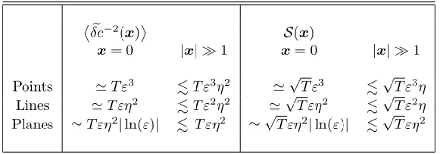
We also present a detailed analysis of the behavior of the two imaging functionals when trying to locate singular perturbations in the velocity of propagation and in the high fre-quency regime. Three different kinds of perturbations (points, lines and surfaces) are con-sidered to prove that the typical contrast seen in the image strongly depends on the type of perturbation. We perform a detailed resolution and stability analysis. Quantitative results show that point singularities are easily seen, and surface singularities are the hardest to locate.
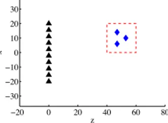
Finally, some possible applications of our approach with simultaneous random sources are investigated and we elaborate on the fascinating fact that imaging with simultaneous sources of the two types we have described gives a resolution that corresponds to the one obtained in the classical setting, where the recordings of the responses at all of the receivers are available for each experiment (corresponding each time to a new source emitting the signal). Simple numerical results are shown to support this fact.
The results concerning the high frequency analysis of the imaging functional are contained in the preprint [Fe12b]. The remaining sections, namely the description of the imaging algorithm using the simultaneous random sources described, its statistical stability and the results contained in the final section on applications and simulations are taken from the joint work [DFGS12] with M. De Hoop, J. Garnier and K. Sølna published in Contemporary Mathematics.
1.3
The stochastic linear transport equation:
regulariza-tion by noise.
The possibility that noise may prevent the emergence of singularities is an intriguing phe-nomenon that is under investigation for several systems. A number of equations have been studied with respect to this question, providing both positive and negative examples. In
general, regularization effects are more easily achieved with a multiplicative noise term, so that we shall restrict our analysis to this case.
In chapter 4 we provide a positive example showing that for the linear transport equa-tion under very weak assumpequa-tions on the drift coefficient (we only require some degree of integrability) and in the presence of a multiplicative noise term, some degree of regularity of the initial condition is maintained. In particular, discontinuities cannot appear. This fact follows from a representation formula which expresses the solution in terms of the initial condition composed with a stochastic flow. In previous works [FF11, FF12a] we had ana-lyzed the solution of the stochastic differential equation (SDE) that generates this flow and proved some important regularity properties. In particular, the flow is α-Hölder continuous for every α ∈ (0, 1), with probability one, and is differentiable in some weak sense. It follows that the solution starting from a regular initial condition remains at least Hölder continuous, so that no discontinuity can appear.
The description of the class of functions in which we look for solutions of the stochastic transport equation is quite technical, and is given by definition 4.6. We call a solution in this class a weakly differentiable solution. Existence of a weakly differentiable solution under our weak integrability assumptions on the drift coefficient is proved in theorem 4.10 by showing that the representation formula described above provides a solution. And by theorem 4.11 this fairly regular solution is also unique.
The results presented in this chapter are mainly contained in the preprint [FF12b], which is a joint work with F. Flandoli. Some necessary technical results from the previous joint works [FF11, FF12a] are also presented in appendix A.
Noise and solitons
A solution of a nonlinear dispersive equation modelling the propagation of waves may show two components with a very distinct behavior. The radiation component is the one whose amplitude decays in time as a power law due to dispersive effects, which refers to the fact that the speed of the waves can vary according to frequency. For many nonlinear systems, a delicate balance between the dispersive and nonlinear effects may occur, producing stable waves. They are referred to as the soliton component of the solution (solitons, in short). Soli-tons are stable, solitary waves with elastic interactions (the only effect of a collision between two solitons is a phase shift). Stable refers to the fact that they propagate over arbitrarily large distances with constant velocity and profile. The identification of the soliton compo-nents is therefore essential to characterize the long-time behavior of the solution of the PDE. Examples of exactly solvable models which can produce solitons are the Korteweg - de Vries (KdV) equation, the nonlinear Schrödinger (NLS) equation and the sine -Gordon equation, the Kadomtsev-Petviashvili equation, the Toda lattice equation, the Ishimori equation, the Dym equation, etc.
Historically, solitons were first observed by John Scott Russell during the first half of the 19th century [Ru1], [Ru2]. His observations dealt with stable water waves in a narrow
channel. A lot of research followed, until Diederik Korteweg and Gustav de Vries proposed in 1895 what is now known as the KdV equation to model the propagation of waves in shallow waters [KV1]. This model also explains mathematically the existence of stable solitary waves. But it was only much later, in 1967, that a new technique allowing to find analytical solutions of the KdV equation was discovered by Gardner, Greene, Kruskal and Miura [GG67]. It is the inverse scattering transform (IST), which thanks to the successive work of Lax [La68] allows to treat analytically many soliton-generating systems, including the NLS equation.
Today, solitons still attract a lot of research which has potentially substantial applica-tions in many fields. For example, in a fiber optic system one can exploit the solitons’ inherent stability to improve long-distance transmission and increase the performance of optical telecommunications. Another broad domain in which soliton solutions appear is in water waves propagation, for both surface and internal waves.
One important field of research regards the effects of noise on solitons. Noise can be introduced in different ways, to account for different physical effects. For example, one can add an additive or multiplicative noise term in the equation to model some random forcing or external potential. Soliton dynamics for the KdV equation under random forcing, modeled by the addition of an additive noise term in the equation, has been analyzed in [dBD07]
while the case of solitons of the KdV equation with a potential given by a multiplicative noise term is studied in [dBD09]. Numerical results for these two kinds of random perturbations are presented in [SRC98] and [DP99]. Corresponding numerical and analytical results for the random NLS equation are presented in [FKLT01, DdM02b].
Another way to introduce random perturbations using a deterministic equation is to use random initial conditions. In this chapter we shall consider this approach and study how the introduction of noise in the initial condition affects solitons. We focus on two examples of nonlinear PDEs, the NLS and the KdV equations. They are completely integrable sys-tems, widely employed in different fields to model nonlinear and dispersive effects in wave propagation. The (one - dimensional) NLS equation
∂U ∂t + i 2 ∂2U ∂x2 + i|U| 2U = 0 (2.0.1)
models in particular short pulse propagation in single -mode optical fibers (then, t is a propagation distance and x is a time) [MN]. The electromagnetic wave propagating in the fiber is the solution U(t, x), which is a complex function. The NLS equation is also used to model the profile of the amplitude of wave groups for surface water waves: envelope solitons in deep waters approximately solve this equation [Za68]. The NLS equation is also used in the context of Bose -Einstein condensate theory, as the general time dependent Gross -Pitaevskii equation producing the wavefunction of a single particle immersed in the Bose -Einstein condensate reduces to the NLS equation is the absence of an external potential [PS].
The KdV equation ∂U ∂t + 6 U ∂U ∂x + ∂3U ∂x3 = 0 (2.0.2)
has been used since 1895 to model shallow water waves propagation [Wh], and recently it has also found applications in many other physical contexts, such as plasma physics [ZK65], internal waves (both in water and air) [AS], [Mi79], and many others [AC].
An effective method to deal with both equations is the Inverse Scattering Transform (IST), a powerful tool to study solutions of completely integrable nonlinear equations, see [APT]. In this framework, the problem is transformed into a linear system of differential equations where the initial condition enters as a potential and soliton components corre-spond to discrete eigenvalues. Our approach to both examples relies on this machinery.
The first result we obtain is that for the NLS and KdV equations the study of soliton emergence from a localized, bounded initial condition perturbed by a wide class of rapidly oscillating random processes can be reduced to the study of a canonical system of stochastic differential equations (SDEs), formally corresponding to the white noise perturbation of the initial condition [Fe12a]. The integrated covariance is the only parameter of the perturbation process that influences the limit system of SDEs. This is the main result of section 2.1.
In section 2.2 we study this limit system to obtain quantitative information on the stability of solitons with respect to small random perturbations in different settings: one can consider real or complex random perturbations (for NLS), with or without a background deterministic initial condition (for KdV).
Finally, in the last section we collect a few examples of different random initial conditions for the nonlinear Schrödinger equation and present the different techniques needed to treat them. We can describe different effects on the soliton generation according to the nature of the random process used as initial condition. For rapidly oscillating real processes we study the threshold of the length of the support of the initial condition needed to create the first soliton and show that it is almost surely finite. For other examples with complex initial
conditions we can show that the probability of creating solitons with any given velocity is zero. We then turn our attention to the density of the distribution of the velocity and amplitude of solitons created by complex random initial conditions. A formula for the limit case of rapid oscillations has been recently obtained [KM08]; we will explicit the computation needed to obtain this formula and the correction terms for fast, but not infinitely rapid, oscillations, in the practical example of a Ornstein-Uhlenbeck process and detail the scheme to apply for a general class of rapidly oscillating Markov processes.
Notation
We introduce some general notation used throughout the chapter. Further specific notation used only in a single passage are introduced when needed.
If z ∈ C is a complex number, we denote �[z] its real part and �[z] its imaginary part. z∗
denotes the complex conjugate of z. In particular, ζ is used to denote the complex number which will be associated to each soliton; we shall write it as ζ = ξ + iη.
For a vector x ∈ Rd or x ∈ Cd, we will write xT to denote the transposed vector and
x = (x1, x2, ...) to indicate its coordinates. The vectors e1= (1, 0, ...), e2= (0, 1, ...) always
refer to the elements of the canonical basis of Rd (or Cd). We will use B
r(x) to denote the
ball of radius r centered in x. We will use |·| to denote either the absolute value or the norm in Rd or Cd. For norms defined on other spaces, and in particular on functional spaces, we
will use � · �.
We will use subscripts to denote the dependence of constants on the parameters of the problem, as in CR.
For functional spaces, we use the notation X(A; B), where X denotes the regularity of the functions, A indicates the domain and B the space in which the functions take values. For example, C0denotes a space of continuous functions, C1a space of continuously differentiable
functions, Lp the space of p-integrable functions and Wl,kis used to denote Sobolev spaces.
Finally, f � g denotes the convolution product between f and g.
2.1
Rapidly oscillating random perturbations
We consider in this section the case of initial conditions perturbed with a rapidly oscillating random process. We prove that for both the NLS and KdV equations the behavior of the soliton components of the solution actually shows very little dependence on the kind of perturbation, the limit behavior being controlled by a canonical system of SDEs where the only parameter of the original perturbation playing a role is its integrated covariance.
Explicit computations are presented in the case of a square (box-like) initial condition perturbed with a zero mean, stationary, rapidly oscillating process νε(x) := ν(x/ε2):
U0(x) = � q +σ ενε � [0,R](x) , (2.1.1)
but they can be extended to the case of perturbation of a more general initial condition defined by a bounded, compactly supported function q(x). The rapidly oscillating fluctua-tions of the initial condition can model the high-frequency additive noise of the light source generating the pulse in nonlinear fiber optics, for instance.
We will show in subsection 2.1.2 that for rapidly oscillating processes (small values of ε) the limit system governing the stability of the soliton components reads as a set of SDEs
and it is formally equivalent to the system where the initial condition contains a white noise ( ˙W ) perturbation U0(x) = � q +√2α σ ˙Wx � [0,R](x) , (2.1.2)
where α is the integrated covariance of the process ν. This shows that to study the soliton components in the limit of rapid oscillations, the only required parameter of the statis-tics of ν is its integrated covariance. Notice however that we cannot directly use a white noise to perturb the initial condition, as the IST requires some integrability conditions on the initial condition (for example, U0∈ L1for NLS), which are not satisfied by a white noise.
2.1.1
The Inverse Scattering Transform method
The essential technical instrument we will use to deal with the two nonlinear evolution equa-tions we analyze is the inverse scattering transform. This method is a non-linear analogue of the Fourier transform, which can be used to solve many linear partial differential equations. The basic principle is the same, and with both methods the calculation of the solution of the initial value problem proceeds in three steps, as follows:
1. the forward problem: the initial conditions in the original “physical” variables are transformed into some spectral coefficients. For the Fourier transform they are simply the Fourier coefficients, while for the IST they are called scattering data. These scattering data characterize a spectral problem in which the initial conditions play the role of a potential. The Jost coefficients (a, b) together with the set of the discrete eigenvalues (ζn) of the spectral problem and the associated norming constants ρn
compose the set of scattering data.
2. time dependence: the Fourier coefficients or the scattering data evolve according to simple, explicitly solvable ordinary differential equations. It is easy to obtain their value at any future time.
3. the inverse problem: the evolved solution in the original variables is recovered from the evolved solution in the transformed variables. This is done using the inverse Fourier transform or solving the Gelfand-Levitan-Marchenko equation (for the IST).
The direct transform (direct scattering problem) consists in the analysis of the spectrum of an associated operator L, where the initial condition U0enters as a potential. The explicit
form of the operator L(U0) for NLS and KdV together with its domain are given below. L
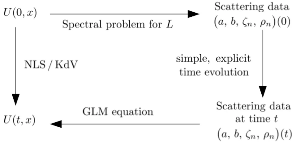
is known as the first operator of the Lax pair. From the eigenvalues and corresponding eigenfuctions of the operator L one can construct the Jost coefficients a(ζ, t) and b(ζ, t) at t = 0. The essential point is that the scattering data, which is to say the Jost coefficients together with the discrete spectrum and the norming constants associated to each discrete eigenvalue, contain enough information to completely characterize the function U. Moreover, the evolution of the Jost coefficients is very simple: it is governed by the second operator of the Lax pair, M, which is a linear differential operator. Finally, the inverse transform consist in the reconstruction of the solution U(t, x) from the scattering data at time t. This is done by solving an integro-differential equation known as the Gelfand-Levitan-Marchenko equation. The principle of this method is schematically illustrated in figure 2.1.
The IST is a very efficient method to solve the initial value problem for many nonlinear evolution equations, but it can be used for other purposes too. For example, one can construct special solutions by posing an elementary solution in the transformed variables and applying the inverse transformed to obtain the corresponding solution in the original variables. Or, and this is how we will use it, one can study the Jost coefficients to see if a special solution, namely a soliton, will appear from a given initial condition. This approach is particularly convenient as solitons have very easy representations in terms of the scattering data: they correspond the discrete eigenvalues, which can be found as the zeros of the function a in the upper complex half-plane. The continuous spectrum, which for KdV and NLS is the real line, corresponds instead to the radiative component of the solution.
IST for NLS
Let us now apply the IST machinery to our first example, the NLS equation. To obtain the scattering data, the Zakharov-Shabat spectral problem (ZSSP) is introduced
� ∂ψ1
∂x = i U0(x) ψ2− iζ ψ1 ∂ψ2
∂x = i U0∗(x) ψ1+ iζ ψ2
, (2.1.3)
where ψnare the components of a vector eigenfunction Ψ and ζ ∈ C is the spectral parameter.
This system is given by the operator
L(U0) = i � 1 0 0 −1 � ∂x+ � 0 U0 −U∗ 0 0 � acting on H1(R) = {Ψ | ψ
i∈ L2(R), ∂xψi∈ L2(R) , i = 1, 2}. When U0= 0, it is easy to see
that the continuous part of the spectrum is composed by the whole real line. The eigenspace associated to the eigenvalue ζ ∈ R has dimension 2 and the functions
Ψ ∼ � 1 0 � e−iζx , Φ ∼ � 0 1 � eiζx
define a basis of this space. In this case, the discrete spectrum of L(0) is empty, because the nontrivial solutions of ∂xf = iζf are not in L2(R).
for ζ ∈ R the solutions Ψ, �Ψ, Φ, �Φ defined by the boundary conditions Ψ ∼ � 1 0 � e−iζx Ψ ∼� � 0 1 � eiζx , x → −∞ (2.1.4) Φ ∼ � 0 1 � eiζx Φ ∼� � 1 0 � e−iζx, x → +∞ (2.1.5)
produce two sets {Ψ, �Ψ} and {Φ, �Φ} of linearly independent solutions. These functions are related through the system
� Ψ � Ψ � = � b(ζ) a(ζ) �a(ζ) �b(ζ) � � Φ � Φ � , (2.1.6)
where ζ ∈ R and a(ζ), b(ζ) are the Jost coefficients (at time zero). They satisfy |a|2+|b|2= 1.
The functions Ψ and Φ are called Jost functions. If U0∈ L1(R), the function a(ζ) can be
continuously extended to the upper complex half-plane in a unique way, and the extended function is analytical for �[ζ] > 0 (this extension is analytical if we require some additional fast-decay conditions on the initial condition, such as exponential decay), see [APT, Lemma 2.1]. Then, one can show that the extension of the Jost coefficient a(ζ) to the upper complex half-plane can only have a finite number of simple zeros. If ζn is a zero of a, then Ψ and
Φ are linearly dependent, so that there exists a coefficient ρn for which Ψ = ρnΦ. The
eigenfunction corresponding to this spectral value is bounded and decays exponentially, so that ζn turns out to be an element of the discrete spectrum.
The scattering data evolve according to very easy and uncoupled equations: ∂ta(ζ, t) = 0 , ∂tb(ζ, t) = −4iζ2b(ζ, t) , ∂tρn(t) = −4iζn2ρn(t) ,
and the discrete spectrum (ζn)n=1...N does not evolve.
The NLS equation presents an infinite number of quantities that are conserved (as soon as they are well defined) during the evolution [MNPZ]. We shall present here two of them which are of special physical interest.
Mass: The mass of a wave is defined as N =�R|U|
2dx. It can be obtained from the scattering
data using the formula
N =� n 4ηn− 1 π � R ln�|a(ζ)|2�dζ ,
where ηnis the imaginary part of a discrete eigenvalue ζn. From this expression one sees
how the total mass easily decomposes into the sum of two contributions, one coming from the soliton components of the solution, Ns = �n4ηn, the other (the integral
over the continuous spectrum, Nr) carried by the radiative part of the solution.
Energy: The energy (which is also twice the Hamiltonian) of a wave is given by the formula E =�R|∂xU |
2− |U|4dx. It can be obtained from the scattering data as follows:
E =� n 8i 3 � (ζn∗)3− (ζn)3�− 4 π � R ζ2ln�|a(ζ)|2�dζ .
Also the total energy decomposes into the sum of two contributions. Each soliton contributes with an energy of (8i)/3 ∗�(ζ∗
n)3− (ζn)3
�
part of the solution provides an energy of −4/π�Rζ
2ln�|a(ζ)|2�dζ.
Each discrete eigenvalue ζ = ξ + iη, η > 0 corresponds to a soliton component of the solution. A pure soliton solution of the NLS equation has the form
U (t, x) = 2iη
exp�− 2iξ(x − x0) − 4i(ξ2− η2)t
�
cosh�2η(x − x0+ 4ξt)
� . (2.1.7)
The amplitude of the soliton only depends on the imaginary part of the discrete eigenvalue associated, and is given by 2η. The mass of the soliton is 4η, according to the above definition. The speed of the soliton is determined by the real part of the eigenvalue, and is given by 4ξ. The energy of the soliton depends on both the real and imaginary part of the eigenvalue: Es= 16η � ξ2−1 3η 2�.
The pure soliton solution (2.1.7) is associated to the eigenvalue ξ + iη and the scattering data a(ζ, t) = ζ− ζn ζ− ζ∗ n , b(ζ, t) = 0 , ρ(t) = η ξ+ iη exp �
− 2i(ξ + iη + π/4) − 4i(ξ + iη)2t�.
IST for KdV
Let us now consider the KdV equation. If we assume some integrability of the initial condi-tion, namely U0∈ P1:= � f : R → R � � � � ∞ −∞ �1 + |x|���f(x)��dx < ∞� , (2.1.8) it is possible to introduce a direct scattering problem associated to the KdV equation [AC], which is given by the first operator of the Lax pair acting on H2(R) =�f ∈ L2(R) | ∂2
xf ∈
L2(R)�, and reads
∂2ϕ
∂x2 + (U0+ ζ
2)ϕ = 0 . (2.1.9)
The continuous part of the spectrum of equation (2.1.9) is again the real axis. For ζ ∈ R, there are two convenient complete sets of bounded functions associated to equation (2.1.9), defined by their asymptotic behavior:
φ∼ e−iζx φ�∼ eiζx , for x → −∞ ψ∼ eiζx ψ�∼ e−iζx, for x → +∞ . It follows from the above definitions that
φ(x, ζ) = �φ(x, −ζ) , ψ(x, ζ) = �ψ(x, −ζ) and � φ � φ � = � b(ζ) a(ζ) �a(ζ) �b(ζ) � � ψ � ψ � ,
where ζ ∈ R and a(ζ), b(ζ) are the Jost coefficients (at time zero). They satisfy |a|2−|b|2= 1.
The function a can be continuously extended to an analytical (for �[ζ > 0]) function in the upper complex half-plane, where it has only a finite number of simple zeros located on the imaginary axis ζ = iη, see [AC, Lemma 2.2.2]. Just as for the NLS equation, these zeros turn out to be the eigenvalues of the discrete spectrum, which correspond to the soliton components of the solution. The scattering data evolve according to the uncoupled system
∂ta(ζ, t) = 0 , ∂tb(ζ, t) = 8iζ3b(ζ, t) , ∂tρn(t) = 8iζn3ρn(t) ,
and the discrete spectrum (ζn= iηn)n=1...N does not evolve.
Also the KdV equation has an infinite number of conserved quantities. The first two of them are called the mass and energy of the solution and are defined below, [Ga01].
Mass: The mass of a wave is defined as N =�RU dx. It can be obtained from the scattering
data using the formula
N =� n 4ηn− 1 π � R ln�|a(ζ)|2�dζ ,
where ηn is the imaginary part of a discrete eigenvalue ζn. Each soliton component
of the solution contributes with a mass of 4ηn, while the term given by the integral
over the continuous spectrum in the above equation represents the contribution to the total mass due to the radiative part of the solution.
Energy: The energy is given by E =�RU
2dx, and it can be obtained from the scattering data
using the formula
E =� n 16 3 η 3 n+ 4 π � R ζ2ln�|a(ζ)|2�dζ .
The total energy decomposes into the sum of two terms, one taking into account the contribution of each soliton component (16η3
n/3), the other accounting for the energy
of the radiative part of the solution (the integral over the continuous spectrum). Each discrete eigenvalue ζ = iη, η > 0, corresponds to a soliton component of the solution. A pure soliton solution is given by
U (t, x) = 2η2sech2�
η(x − x(t))�, (2.1.10) where x(t) = x0+ 4η2t is the center of the soliton. As one can see from this equation, the
amplitude 2η2and speed 4η2 of the solitons of the KdV equation are linked. The mass of a
soliton is N = 4η and its energy E = 16η3/3. The soliton solution (2.1.10) is associated to
the eigenvalue iηn and the scattering data
a(ζ, t) = ζ− iη
ζ+ iη , b(ζ, t) = 0 , ρ(t) = 2ηe
2ηx0e8η3t.
2.1.2
Limit of rapidly oscillating processes
This subsection contains a rigorous justification for the use of the IST. We have already remarked that to be able to apply the IST the initial condition U0 needs to satisfy some
integrability condition, L1 for NLS and (2.1.8) for KdV. These hypotheses are satisfied by
initial conditions of the form (2.1.1) for any ε > 0 if ν is bounded. Our objective is to show that the IST applied to these random initial conditions gives a problem that reads as a
canonical system of SDEs in the limit ε → 0. Thanks to the convergence result of Theorem 2.2 below, this limit system can be used to study the behavior of rapidly oscillating initial conditions (0 < ε � 1), as we shall do in the following sections. We stress that our interest is in the study of rapidly oscillating initial conditions, which are physically more relevant than the limit case of infinitely rapid oscillations and for which the IST can be applied in a rigorous way. We make the following assumptions (standard in the diffusion approximation theory, [FGPS]) on the process ν:
Hypothesis 2.1. Let ν(x) be a real, homogeneous, ergodic, centered, bounded, Markov stochastic process, with finite integrated covariance�0∞E[ν(0)ν(x)] dx = α < ∞ and with generator Lν satisfying the Freedholm alternative.
Set Uε 0(x) := � q +σ εν(x/ε 2)� [0,R](x) (2.1.11)
and remark that for x ∈ [0, R] � x 0 U0ε(y) dy ε→0−→ � x 0 U0(y) dy = qx + √ 2α σWx
in the space of continuous functions C0�[0, R]; R�, in distribution, see [FGPS]. For every
ε > 0, we apply the first step of the IST to the NLS and KdV equations with the initial condition Uε
0, to obtain the associated spectral problem. Then we will investigate the passage
to the limit of this problem. We point out that this passage to the limit is quite delicate: if it is relatively easy to obtain a pointwise (in ζ) convergence of the spectral data, to obtain fine results for the limit case and for situations near the limit case (0 < ε � 1), a much stronger convergence will be needed.
NLS: pointwise convergence
We consider the ZSSP system associated to the NLS equation: our goal is to identify the points of the upper complex half-plane, ζ ∈ C+, for which there exists a solution Ψ of the
first order system (2.1.3) for x ∈ [0, R], satisfying the boundary conditions
Ψ(0) = � 1 0 � and ψ1(R) = 0
derived from the exponential decay conditions (2.1.4). These particular values of ζ are the discrete eigenvalues of the ZSSP and correspond to the soliton components of the solution. The strategy employed is to consider the flow Ψ(x, ζ), x ∈ [0, R], ζ ∈ C+, solution of (2.1.3)
with initial condition
Ψ(0) = � 1 0 � , (2.1.12)
and look for the values of ζ for which the final condition is satisfied.
For a fixed value of ζ, we consider the solution Ψε of the ZSSP obtained from the
application of the first step of the IST method: ∂ψε1 ∂x = −iζ ψ1ε+ i U0ε(x) ψε2 ∂ψε 2 ∂x = i � Uε 0(x) �∗ψε 1+ iζ ψ2ε , (2.1.13)
with initial condition Ψε(0) = � 1 0 � .
Now, [FGPS, Theorem 6.1] states that the process Ψεconverges in distribution in C0([0, R]; C2)
to the process Ψ solution of � dψ1=�(−iζ − ασ2) ψ1+ iq ψ2�dx + i √ 2α σψ2dWx dψ2= � i q ψ1+ (iζ − ασ2) ψ2 � dx + i√2α σψ1dWx (2.1.14)
with initial condition (2.1.12), which can be rewritten in Stratonovich form as
dΨ = i � −ζ q q ζ � Ψ dx + i√2α σ � 0 1 1 0 � Ψ ◦ dWx . (2.1.15)
For NLS we can also consider perturbations produced by a complex process: let ν1, ν2
be two independent copies of the process ν and set �ν := ν1+ iν2. One can define U0εusing �ν
instead of ν; proceeding as above, from the IST one obtains again the system (2.1.13), and from [FGPS, Theorem 6.1] one gets that in this case the limit process is the solution of
dΨ = i � −ζ q q ζ � Ψ dx + i√2α σ � 0 1 1 0 � Ψ ◦ dWx(1)− √ 2α σ � 0 1 −1 0 � Ψ ◦ dWx(2), (2.1.16)
where the W(i) are two independent Wiener processes, with the same initial condition
(2.1.12).
KdV: pointwise convergence
We apply the same strategy to the KdV equation: the goal is to obtain the values of ζ ∈ C+
for which there exists a solution ϕ of
ϕεxx+ (U0ε+ ζ2)ϕε= 0 (2.1.17)
with the boundary conditions
ϕε(0) = 1 , ϕεx(0) = −iζ , ϕεx(R) − iζϕε(R) = 0 .
These conditions correspond to imposing exponential decay of the solution at infinity. Set-ting Φ := (ϕ, ϕx)T this equation can be transformed into
dΦε= � 0 1 −Uε 0 − ζ2 0 � Φεdx (2.1.18) with boundary conditions
Φε(0) = � 1 −iζ � , φε2(R) − iζφε1(R) = 0 .
We consider the flow Φε(x, ζ), x ∈ [0, R], ζ ∈ C+, defined by the above equation with only
Again by [FGPS, Theorem 6.1], Φε converges in distribution to the solution of dΦ = � 0 1 −q − ζ2 0 � Φ dx +√2α σ � 0 0 1 0 � Φ dWx (2.1.19)
which, in terms of the function ϕ, can be rewritten as dϕx= −(q + ζ2) ϕ dx +
√
2α σϕ dWx. (2.1.20)
The initial condition is
Φ(0) = � 1 −iζ � , or equivalently ϕ(0) = 1 , ϕx(0) = −iζ . (2.1.21)
Remark that in the last two differential equations above the Stratonovich and Itô stochastic integrals coincide.
Convergence as C1 functions
The convergence obtained above is only for a (finite number of) fixed ζ and σ, but we can do much better. Indeed, in the next section we will need to differentiate the limit process with respect to the parameters (ζ, σ), so that we look for a convergence in C0�[0, R]; C1(R3)�. This
is the main result of this section; the exact formulation is given in the following theorem. We will focus on the problem of finding the values of ζ for which the limit flows Ψ and Φ match the final conditions in section 2.2.
Theorem 2.2. Assume hypothesis 2.1 and define Uε
0 as in (2.1.11). Let Ψε:= (ψε1, ψ2ε)T be
the solution of (2.1.13) with initial condition (2.1.12) and Ψ the solution of (2.1.15) with the same initial condition. Let also ϕεbe the solution of (2.1.17) with initial condition (2.1.21)
and ϕ be the solution of (2.1.20) with the same initial condition. Considering these as functions of the space variable x and the parameters ξ, η, σ, we have in the limit of ε → 0 that Ψε(x, ξ, η, σ) → Ψ(x, ξ, η, σ) weakly in C0�[0, R]; C1(R3; C2)�and ϕε(x, ξ, η, σ) → ϕ(x, ξ, η, σ)
weakly in C0�[0, R]; C1(R3; R)�.
To prove this theorem we need a standard tightness criteria, provided by the two following lemmas [Me]. We will use D�[0, R]; E�to denote the space of CadLag processes defined for x ∈ [0, R] and with values in the space E. The first lemma is due to Aldous, [Al78]. Lemma 2.3. Let (E, d) be a metric space, and Xεa process with paths in D�[0, R]; E�. If
for every x in a dense subset of [0, R] the family�Xε(x)�
ε∈(0,1] is tight in E and X
ε satisfy
the Aldous property:
A : For any κ > 0, λ > 0, there exists δ > 0 such that lim sup
ε→0 τ <Rsup
sup
0<θ<δ∧(R−τ )
P��Xε(τ + θ) − Xε(τ )� > λ�< κ ,
where τ is a stopping time; then the family�Xε�
ε∈(0,1] is tight in D
�
[0, R]; E�.
If H is a Hilbert space and Hna subspace of H, we shall use πHnto denote the projection
of H onto Hn. Also, dHis used to denote the distance on H introduced by the inner product.
Lemma 2.4. Let H be a Hilbert space and Hnbe an increasing sequence of
finite-dimensio-nal subspaces of H such that, for any h ∈ H, limn→∞πHnh = h. Let (Z
ε)
ε∈(0,1] be a family
of H-valued random variables. Then, the family (Zε)
ε∈(0,1] is tight if and only if for any
κ> 0 and λ > 0, there exist ρκ and a subspace Hκ,λsuch that
sup
ε∈(0,1]
P��Zε� ≥ ρκ�≤ κ and sup
ε∈(0,1]
P�dH(Zε, Hκ,λ) > λ�≤ κ . (2.1.22)
Proof of Theorem 2.2. To unify notation, we shall use Xεto denote both Ψεand Φε.
There-fore, Xεis the solution of what we shall call the approximated system, which is either system
(2.1.13) or (2.1.18), with ε > 0.
Since propositions 2.14 and 2.21 ensure that the limit equations for Ψ and Φ have a unique solution which is C0�[0, R]; C1(R3)�, it suffices to prove convergence in the space of
CadLag processes D�[0, R]; C1(R3)�. We will do so in three steps.
Steps 1 contains a technical result needed for the application in step 2 of lemma 2.4, namely the proof of the bound (2.1.23).
In step 2, using lemma 2.4, we will show that for every fixed x the sequences�Ψε(x)� εand � Φε(x)� ε, denoted � Xε(x)�
ε in the following, are tight in the Hilbert space H := W 3,2(G).
Note that, by Sobolev imbedding, H �→ C1(G). Here, G is an open, bounded subset of R3,
the space of parameters. For simplicity we take G = (−N, N)3for some real positive constant
N ; a justification of the fact that it is not restrictive to assume that the set of parameters G is bounded is given below in the proof of proposition 2.14, where the convergences we are proving here will be used.
In the last step we will use lemma 2.3, where we take E to be the Hilbert space H. This will provide the desired convergence of the family of processes (Xε)
ε∈(0,1] in
D�[0, R]; C1(R3)�.
Since Xε is the solution of a linear differential equation with coefficients smooth in the
parameters µ = (ξ, η, σ), from the explicit formula for the solution we get that Xε(x, µ) is
smooth in the parameters. We will soon use its derivatives in the parameters: the vector of Xε and its first derivatives in µ still satisfy a linear system of ODEs whose coefficients
depend linearly on the parameters and on the process ν(x/ε2), and the same result holds
adding higher order derivatives.
Step 1 (A preliminary estimate). The key point to show that �Xε(x, µ)�
µ∈G is tight in
H = W3,2(G) for every x ∈ [0, R] is the proof of the bound
lim sup ε→0 E���Xε(x, ·)�� W6,2(G) � ≤ C < ∞ (2.1.23)
uniformly in x ∈ [0, R]. This is the content of this step.
Define Yε as the vector process of Xε and all of its derivatives in the parameters µ =
(ξ, η, σ) up to order 6. As remarked above, this process is the solution of a linear system of ODEs with coefficients (the matrices M1 and M2) linear in the parameters:
d dxY ε= M 1Yε+ 1 εν(x/ε 2)M 2Yε.
Since G is bounded, we only need to check that the second moment of Yε(x, µ) is uniformly
bounded with respect to ε ∈ (0, 1], µ ∈ G and x ∈ [0, R]. Actually, we aim at a stronger result, which we will need later. We are going to show that (recall that Y0= Y0ε is
for x ≤ 0, which is deterministic, and the boundary condition at x → −∞) E� sup x∈[0,R] � �Yε(x)��2�≤ C R � 1 +��Y (0)��2�< ∞ . (2.1.24)
Following [FGPS, Section 6.3.5], we show this bound with the perturbed test function method. Let Lε be the infinitesimal generator of the process Yε and L the infinitesimal
generator of the process Y obtained from the process X solution of the limit system (2.1.15) or (2.1.19). Let m ∈ N be such that Yε(x) ∈ Cm and let K be a compact subset of R
containing the image of the bounded process ν. For every y ∈ Cm and z ∈ K, Lε has the
form Lεg(y, z) = 1 ε2Lνg(y, z) + z ε � M2y �T ∇yg(y, z) + � M1y �T ∇yg(y, z) ,
where Lν is the infinitesimal generator of the process ν, as defined in hypothesis 2.1. Let
f be the identity function on Cm and fε(y, z) = y + εf
1(y, z) be the associated perturbed
function, which is solution of the Poisson equation Lνf1(y, z) = −z�M2y� T
∇yf (y). In this
equation, y plays the role of a frozen parameter, so that f1has linear growth in y, uniformly
in z, and the same holds for
Lεfε(y, z) = z�M2y �T ∇yf1(y, z) + ε � M1y �T ∇yf1(y, z) . Since Yε(x) = Yε(0) − ε�f1�Yε(x), νε(x)�− f1�Yε(0), νε(0)�� + � x 0 L εfε�Yε(x�), νε(x�)�dx�+ Mε x, where Mε
x is a vector valued martingale, we get the bound
sup
x∈[0,R]
�
�Yε(x)�� ≤��Yε(0)�� + εC�1 + sup x∈[0,R] � �Yε(x)��� + C � R 0 1 + sup x�∈[0,x] � �Yε(x�)�� dx + C sup x∈[0,R] � �Mε x � � . For ε ≤ 1
2C, applying Gronwall’s inequality and renaming constants we get
sup x∈[0,R] � �Yε(x)�� ≤ C R � 1 +��Yε(0)�� + sup x∈[0,R] � �Mε x � ��. (2.1.25)
The quadratic variation of the martingale is given by
�Mε�x= � x 0 gε�Yε(x�), νε(x�)�dx�, where gε(y, z) =�Lεfε2− 2fεLεfε�(y, z) =�L νf12− 2f1Lνf1 � (y, z) + 2εz��M2y �T f1(y, z) − � M2y �T� (∇yf1)Tf1 � (y, z)� + 2ε2��M1y� T f1(y, z) −�M1y� T� (∇yf1)Tf1�(y, z) �
has quadratic growth in y uniformly in z ∈ K. Therefore, by Doob’s inequality, E� sup x∈[0,R] � �Mε x � �2� ≤ C E��Mε�R�≤ C � R 0 1 + E���Yε(x)��2� dx .
Substituting into the expected value of the square of (2.1.25) and using again Gronwall’s inequality, we get (2.1.24), which gives (2.1.23).
Step 2 (Tightness of Xε(x)). In this step we show how to obtain the tightness of the
family�Xε(x, µ)�
µ∈Gfrom (2.1.23) using lemma 2.4. Indeed, from this bound the first part
of condition (2.1.22) follows by the Markov inequality if we take ρκ = C/κ. This bound
also provides information on the regularity of Xε(x), which can be used to prove the second
part of condition (2.1.22) as follows. By the Sobolev imbedding W6,2(G) �→ C4(G) the
bound (2.1.23) implies that Xε ∈ C4(G). An appropriate sequence of subspaces (H n)n is
constructed in the appendix in lemma 2.48, and lemma 2.49 states that for any function g ∈ C4(G) there exists an arbitrarily good approximation g
n belonging to some Hn. The
control on the distance between g and the subspace Hn only depends on the norm �g�C4, so
that by (2.1.23) the approximation is uniform in ε. This provides the second part of condition (2.1.22). Finally, corollary 2.50 provides the last hypothesis of lemma 2.4, namely that for the sequence of subspaces Hn constructed in lemma 2.48, for any h ∈ H, limn→∞πHnh = h.
Then, lemma 2.4 gives that for every x, the family�Xε(x, µ)�
µ∈Gis tight in H = W 3,2(G).
Step 3 (Tightness of Xε). Thanks to lemma 2.3, the tightness of the family of processes
Xεin D�[0, R]; H�follows if we show that the Aldous property [A] holds. Since G is bounded,
we can prove the Aldous property showing that
lim
δ→0 lim supε→0 µ∈Gsup
sup
τ ≤R
sup
0<θ<δ
E���Yε(τ + θ, µ) − Yε(τ, µ)��2�= 0 , (2.1.26) where Yεis the vector process having as components Xεand its derivatives in µ up to the
third order only. We prove the above limit using again the perturbed test function method. With the notations introduced above, we have
� �Yε (τ + θ) − Yε(τ )��2≤ C � � �Mτ +θε − Mτε � � � 2 + C � τ +θ τ � � �Lεfε�Yε(x), νε(x)���� 2 dx + Cε�1 + sup x∈[τ,τ +θ] � �Yε(x)��2� ≤ C � � �Mτ +θε − Mτε � � � 2 + C � τ +θ τ � � �Lεfε�Yε, νε�− Lf(Yε) � � � 2 dx + C � τ +θ τ � �Lf(Yε)��2dx + Cε�1 + sup x∈[τ,τ +θ] � �Yε(x)��2�. We have that E���Mε τ +θ− Mτε � �2� = E��Mτ +θε �2 −�Mτε �2� = E� � τ +θ τ d�M ε �x � .
Since��Lεfε(y, z) − Lf(y)�� ≤ εC(1 + |y|) and |Lf(y)| ≤ C|y|, for θ ≤ δ
E���Yε(τ + θ) − Yε(τ )��2�≤ CR(δ + ε)�1 + E� sup
x∈[0,R]
�
The right-hand side is independent of τ and we can use estimate (2.1.24) to bound it uni-formly in ε and µ. Therefore, (2.1.26) follows and the proof of Theorem 2.2 is complete.
Remark 2.5. Using the notion of pseudo-generators, as introduced in [EK, Section 7.4], it is possible to relax the conditions imposed on the driving process ν(x) assuming that it is just a mixing process instead of Markov.
2.2
Stability of solitons
This section is devoted to the study of the stability of solitons with respect to rapidly os-cillating random perturbations of the initial condition. Our results state that solitons of both the NLS and KdV equation are stable under perturbations of the initial condition. Moreover, for small-amplitude random perturbations, we provide an easy way to compute first order correction terms for the parameters characterizing the solitons. However, if for both equations solitons are stable, a few interesting differences must be pointed out. For example, for NLS there is a thresholding effect for the creation of solitons from noise, so that unless the integral of the deterministic initial condition exceeds a certain threshold, the addition of a small random perturbation cannot generate a soliton. On the other hand, for KdV even a very small random initial condition can produce a soliton. Moreover, we will see that in the presence of a random perturbation KdV solitons are perturbed in both amplitude and velocity, while unless the perturbation is complex the velocity of NLS solitons is not substantially affected.
Thanks to the results of the previous section, we know that for rapidly oscillating initial conditions both the NLS and KdV systems can be investigated using the limit equations (2.1.15) and (2.1.20), which formally correspond to a real or complex white noise perturba-tion on the initial condiperturba-tion.
For NLS we have seen that every soliton is identified by a complex number ζ = ξ + iη such that the flow Ψ(x, ζ) solution of (2.1.15) with initial condition (2.1.12) satisfies also a given final condition. The real and imaginary parts of ζ define the velocity and amplitude of the soliton, respectively. For KdV, solitons are identified by an imaginary number ζ = iη, defining both the velocity and amplitude of the soliton, which are related.
We start analyzing the NLS equation, and leave KdV to the second part of this section. For each of the two equations we start by reporting, in subsections 2.2.1 and 2.2.4, some classical results on the background deterministic solution. Then we analyze how this solu-tion is modified by the introducsolu-tion of a real, small-amplitude, rapidly oscillating random perturbation of the initial condition. This is done in subsections 2.2.2 and 2.2.5. For NLS we can also consider the case of perturbations of the initial condition given by rapidly os-cillating complex processes; the stability of solitons in this case is investigated in subsection 2.2.3. We deal with the limit cases of “quiescent” solitons for NLS and KdV in corollary 2.10, remark 2.18 and proposition 2.20. Finally, for KdV one can also consider the case of a perturbation of the zero initial condition: this is done in subsection 2.2.6.
For simplicity of exposition, in this section we choose the value of the integrated cova-riance of the process ν to be α = 1/2.
2.2.1
NLS solitons – deterministic background solution
Let U0(x) = q [0,R](x). Burzlaff proved in [Bu88] that in this case the number of solitons
generated is the integer part of 1/2+qR/π (see also the relevant discussion and generalization of [Ki89]). They remark how physical intuition suggests that the first soliton created when increasing R corresponds to ζ = 0. This solution is obtained for qR = π/2 and contains a single “soliton” with zero amplitude that they called quiescent soliton. In this case, the velocity of this soliton is also zero. Remark that the quiescent soliton is not a physical soliton, since both its mass and energy are zero. But from a mathematical point of view it could be considered as a soliton, in the sense that it is a bounded solution of the spectral problem corresponding to a zero of the Jost coefficient a. We will also observe that this evanescent soliton is an interesting structure even from a physical point of view, since an infinitesimal random perturbation is sufficient to create (with positive probability) a “true” soliton with positive amplitude.
For values of qR just over the critical threshold of 1/2, the created soliton has zero velocity and nonzero amplitude 2η which can be computed explicitly solving (2.1.3) for pure imaginary values of ζ.
In the first part of this subsection we report some computations relative to this case, as the results and explicit formulas will be used below. We then conclude providing the sketch of an analytical proof of the claimed fact that generated solitons correspond to purely imaginary values of ζ.
For purely imaginary values of ζ = iη, from the decaying condition at −∞ one obtains the initial condition
Ψ(0) = � 1 0 � eηx��� x=0= � 1 0 � . (2.2.1)
The system (2.1.3) for x ∈ [0, R] reads � ∂ψ1
∂x = iq ψ2− iζ ψ1 ∂ψ2
∂x = iq ψ1+ iζ ψ2
and Ψ = (ψ1, ψ2) is a solution of the initial value problem for ζ �= iq if (ζ is imaginary pure)
ψ1(x) = −� iζ q2+ ζ2sin �� q2+ ζ2x�+ cos��q2+ ζ2x�; ψ2(x) = i q � q2+ ζ2sin �� q2+ ζ2x�. (2.2.2)
To be a soliton solution, Ψ needs to satisfy also the decaying condition at +∞, which is to say ψ1(R) = 0. The condition can be rewritten for ζ �= 0 as
f (ζ) = tan(�q2+ ζ2R) + i
� q2+ ζ2
ζ = 0 . (2.2.3) Since a(ζ) = ψ1(R, ζ)eiζR, the function f(ζ) is linked to the first Jost coefficient a(ζ) by the
relation f (ζ) = ia(ζ)e−iζR ζ � q2+ ζ2 cos��q2+ ζ2R� ,
from which we see that the zeros of f coincide with those of a, except for ζ = iq. However, for ζ = iq it is possible to compute explicitly the solution of (2.2.1) satisfying the initial
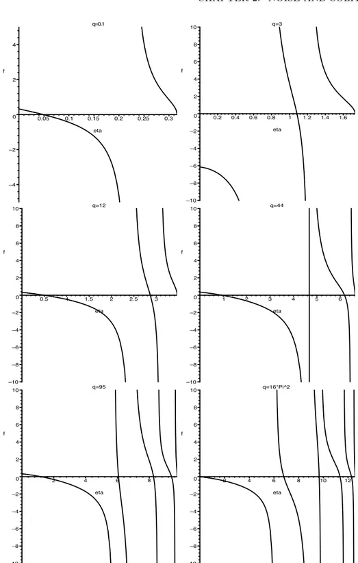
![Figure 3.2: Images given by Kirchhoff migration of the full MSR matrix (a); migration of the data vector obtained with simultaneous sources without random time delays (d); migration of the data vector obtained with blended sources (BS) with random time delays uniformly distributed over [−10, 10] for two realizations of the delays (b,e); migration of the data vector obtained with blended sources with random time delays uniformly distributed over [−100, 100] for two realizations of the delays (c,f).](https://thumb-eu.123doks.com/thumbv2/123doknet/2333931.32348/130.892.169.687.190.517/kirchhoff-simultaneous-uniformly-distributed-realizations-migration-distributed-realizations.webp)
