Dèpartement de Physique
de l’École Normale Supèrieure
Laboratoire de Physique Statistique
THÈSE DE DOCTORAT
DE L’UNIVERSITÉ PARIS 6 – PIERRE ET MARIE CURIE
Spècialitè: Physique des Liquides
prèsentèe par
Peder MØLLER
pour obtenir le grade de
DOCTEUR DE L’UNIVERSITÉ PARIS 6
Sujet de la thèse:
Bandes de cisaillement et la transition
solide/liquide dans les fluides à seuil
( Shear banding and the solid/liquid
transition in yield stress fluids )
Prèvue en 6 octobre 2008 devant le jury composè de :J-L. Barrat Rapporteur
M. van Hecke Rapporteur
M.A.J. Michels Examinateur
P. Coussot Examinateur
E. Clement Prèsident du jury
Acknowledgements
After three years of scientific training and discoveries, my thesis with all its ups and downs has come to an end. Numerous people have helped me achieve this goal and make the downs fewer, the ups more plentiful, and the general process more enjoyable. I owe them my gratitude.
First I would like to thank my supervisor Daniel Bonn for welcoming me into his team, and for letting me benefit from his scientific creativity, enthusiasm, and physical intuition. I have learned a lot from him! Numerous experimental techniques and procedures, but most notably how to leap haphazardly into a complex scientific problem with daring confidence rather than being paralyzed by the challenges.
Secondly I want to thank Sébastien Moulinet for many helpful discussions, showing me experimental techniques, and for running the practical side of the lab in S11 after Daniel moved to Amsterdam. Also the other permanent members of the team; Jacques Meunier, and Anne-Marie Cazabat are thanked for useful discussions.
In addition I wish to thank all the other people that have been part of of the Soft Matter Physics, Instabilities, and Phase Transitions group during my stay here. I have had interesting discussions with all of them, and have learned a lot. Notably I need to thank Nicolas Huang who introduced me to the rheometers and practical rheometrical techniques. In addition I’m especially grateful to Mehdi Habibi, Dirk Aarts, Abdoulaye Fall, Didi Derks, Christophe Chevallier, and Ulysse Delarbre, for countless useful and interesting discussions, exchange of experimental skills, and small experimental collabo-rations that I have enjoyed greatly.
In addition to the scientific acknowledgements I want to thank all those people from the group (and other groups) that I have come to count among my friends for exactly that.
I have also had collaborations and discussions with people from different institutions. I owe thanks to Thijs Michels from Eindhoven University of Technology for providing a model for the viscosity of colloidal aggregates, and for discussions about the modeling of carbopol-like materials. I am also grateful to Stéphane Rodts from the University of Eastern Paris for configuring the MRI setup for measurements on the colloid-salt wa-ter mixture. And I want to thank Jan Mewis from Katholieke Universiteit Leuven for collaboration on the thixotropy of yield stress fluids.
In addition to the people mentioned above, I have had numerous interesting and encouraging discussions with several people at various conferences, and even if I can’t mention all of them here I have enjoyed those discussions as well.
iv Chapter 0. Acknowledgements
I also would like to thank the scientists who have agreed to be members of the jury of my defense for taking their time to examine my work and to contribute with their comments and critique at the defense. I thank the rapporteurs Martin van Hecke and Jean-Louis Barrat, the examinateurs M.A.J. Michels and Philippe Coussot, and the president of the jury Eric Clement.
I am grateful to the EU Framework Programme 6 Marie Curie Research Training Networks scheme (under grant MRTN-CT-2004005728 (PATTERNS)), who have provided the funding for my thesis. I also owe thanks to the institutions that have made my stay here practically possible: Laboratoire de Physique Statistique and its directors during my stay here; Jacques Meunier and Eric Perez, and to Département de Physique de l’Ecole Normale Supérieure and its director Jean-Michel Raimond. And also the Centre National de Recherche Scientifique and Université Paris VI. I also owe thanks to certain people in the LPS for help with technical of administrative tasks. Notably the secretaries Nora, Annie, and Marie, and José and Olivier in the workshop.
Least but certainly not last I’m eternally grateful to a number of people who have not been directly involved in the scientific work during my thesis. Some of these people have helped me a lot along the way, and some of them have been outright essential for me even beginning my thesis, and also for much more important things. First and foremost I need to thank my wonderful and loving family for so many and essential things that I cannot even begin to mention them here. And secondly, I am lucky to have a truly fantastic girlfriend together with whom I came to Paris. Her wonderful company here have turned miserable times into agreeable ones, and agreeable times into happy ones. Finally I want to thank Sid Nagel and Lene Oddershede for being great inspirations as scientists as well as persons.
Contents
Acknowledgements iii
I Introduction to Rheology
1
1 Rheology: The study of non-Newtonian fluids 3
1.1 Introduction . . . 3
1.2 The response of simple materials to an external stress . . . 4
1.3 The flow properties of simple yield stress fluids . . . 4
1.3.1 Flow curves and phenomenological models for simple yield stress fluids . . . 6
1.4 The flow properties of thixotropic yield stress fluids . . . 9
1.4.1 The problems with the yield stress . . . 10
1.4.2 Viscosity bifurcation and avalanche behavior . . . 11
1.4.3 Aging and rejuvenation: A toy-model of a thixotropic fluid . . . 13
1.5 Micro- and mesoscopic models for complex fluids . . . 16
1.5.1 Molecular dynamics simulations . . . 16
1.5.2 Reptation, an example of polymer scaling concepts . . . 16
1.5.3 The SGR model, an example of a mesoscopic model . . . 17
1.6 Granular materials as a complex fluid . . . 18
1.7 This thesis . . . 19
2 Measurement techniques 21 2.1 Introduction . . . 21
2.2 Active rheological techniques . . . 22
2.2.1 The rheometer . . . 22
2.2.2 The Couette, double-gap, and vane-cup geometries . . . 23
2.2.3 Shear banding of simple yield stress fluids . . . 24
2.2.4 The cone-plate geometry . . . 26
2.3 Active rheological tests . . . 26
2.3.1 Shear stress/rate sweep tests . . . 27
2.3.2 Shear strain/stress-relaxation tests . . . 27
2.3.3 Oscillatory sweep tests . . . 27
vi CONTENTS
2.4 Passive measurement techniques . . . 28
2.4.1 Brownian motion . . . 29
2.4.2 Microrheology . . . 29
2.4.3 Dynamic Light Scattering and Diffusing Wave Spectroscopy . . . . 30
2.5 Magnetic Resonance Imaging (MRI) velocimetry . . . 31
II Simple yield stress fluids
35
3 The yielding behavior of simple yield stress fluids 37 3.1 Introduction . . . 373.2 Materials and Methods . . . 39
3.3 Experimental results . . . 39
3.4 A simple physical model for carbopol . . . 43
3.5 Simulation results and comparison to experiments . . . 46
3.6 Discussion of the model and results . . . 48
3.7 General discussion . . . 50
3.8 Conclusion . . . 52
III Thixotropic yield stress fluids
55
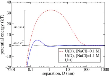
4 What makes a fluid thixotropic 57 4.1 Introduction . . . 574.2 Colloidal interactions: van der Waals forces and Debye lengths . . . 58
4.3 Ludox spheres and salt water . . . 59
5 The negative slope of the flow curve 63 5.1 Introduction . . . 63
5.2 Behavior of the λ-model away from the steady state . . . 64
5.2.1 The evolution of the λ-model under an imposed stress . . . 64
5.2.2 The yield stress measurement problems explained by the λ-model . 66 5.2.3 How to experimentally demonstrate the negative slope of the steady state flow curve . . . 68
5.3 Experimental results . . . 69
5.4 Conclusion . . . 71
6 Shear banding in thixotropic yield stress fluids 73 6.1 Introduction . . . 73
6.2 Some previous shear banding experiments . . . 74
6.3 Shear banding in the λ model . . . 74
6.3.1 Shear banding in heterogeneous stress fields . . . 75
6.3.2 Shear banding in homogeneous stress fields . . . 75
CONTENTS vii
6.4 MRI velocimetry experiments . . . 77
6.4.1 Experimental procedure . . . 77
6.4.2 MRI velocimetry results . . . 78
6.4.3 Experimental demonstration of the lever rule . . . 79
6.5 Comparing the MRI and rheometrical measurements . . . 80
6.5.1 A negative slope in the steady state flow curve can result in a stress plateau under imposed shear rate . . . 81
6.6 Measuring the local state of the material . . . 83
6.6.1 DWS measurements inside and outside the flowing band . . . 84
6.7 A serious limitation of the lever rule . . . 86
6.8 Practical handling of thixotropic yield stress fluids . . . 88
6.9 Conclusion . . . 89
7 A physical model for the rheology of colloids in salt water 91
IV Moist granular materials
95
8 The elastic modulus of moist granular matter 97 8.1 Introduction . . . 978.2 Materials and methods . . . 98
8.3 Experimental results . . . 100
8.4 Predicting the elastic shear modulus of moist granular materials . . . 100
8.5 Discussion . . . 103
8.6 Conclusion . . . 106
9 General conclusion 107
A Numerical code for simulating carbopol 111
B Publications 113
Part I
Introduction to Rheology
Chapter 1
Rheology: The study of non-Newtonian
fluids
Contents
1.1 Introduction . . . 3
1.2 The response of simple materials to an external stress . . . . 4
1.3 The flow properties of simple yield stress fluids . . . 4
1.3.1 Flow curves and phenomenological models for simple yield stress fluids . . . 6
1.4 The flow properties of thixotropic yield stress fluids . . . 9
1.4.1 The problems with the yield stress . . . 10
1.4.2 Viscosity bifurcation and avalanche behavior . . . 11
1.4.3 Aging and rejuvenation: A toy-model of a thixotropic fluid . . 13
1.5 Micro- and mesoscopic models for complex fluids . . . 16
1.5.1 Molecular dynamics simulations . . . 16
1.5.2 Reptation, an example of polymer scaling concepts . . . 16
1.5.3 The SGR model, an example of a mesoscopic model . . . 17
1.6 Granular materials as a complex fluid . . . 18
1.7 This thesis . . . 19
1.1
Introduction
In freshman classical mechanics a physics or engineering student will normally encounter two types of materials (apart from ideal particles and gases): Elastic solids, and Newtonian fluids. An elastic solid is a material that when subject to a force undergoes a total deformation that is proportional to the size of the force. At sufficiently low levels of deformation (and sufficiently short measurement times) all solids are elastic solids and
4 Chapter 1. Rheology: The study of non-Newtonian fluids
some materials (notably rubber) are elastic for large deformations and long times. A Newtonian fluid is a material where the rate of deformation is proportional to the forcing involved. Many of the materials that are ubiquitous in our everyday life are neither elastic solids nor Newtonian fluid however. This is especially true for many foodstuffs like mayonnaise, whipped cream, gels, whipped egg whites, custards etc., which will flow readily like a fluid when stirred with a spoon or savored in the mouth, but will nevertheless keep their shape like a solid if left under only the force of gravity. Rheology is the study of the wealth of such very different materials whose mechanic properties cannot be reduced to either an elastic constant or a viscosity. The behavior of these substances varies greatly, spanning from shear-thinning fluids where the viscosity decreases with the rate of deformation [1–11] over shear-thickening fluids where the viscosity increases abruptly and strongly at high shear rates [1, 2, 6, 7, 12–18], to shake-gels where a fluid is reversibly turned into a solid state when shaken and return to a liquid under rest [19, 20], and strongly thixotropic fluids that do exactly the opposite [21–32]. In this chapter I will present an fundamental introduction to the rheological materials and concepts that are relevant for understanding the subsequent chapters.
1.2
The response of simple materials to an external
stress
Consider the response of an infinite plate of an elastic solid of height, h, subject to a shear stress (the tangential force, F , per unit area, A) of σ ≡ F/A in opposite directions on the two opposing faces as in Fig. 1.1. The external force will deform the material - moving the upper plate some distance d with respect to the lower one - until it is balanced by the elastic response of the material. It is easily seen that if all other parameters are fixed d will be proportional to h, so in order to get a parameter independent of the height of the block the shear strain of the material is defined as γ ≡ d/h. For an elastic solid the shear strain is proportional to the shear stress - it follows Hooke’s law:
σ = G′γ (1.1)
where the constant of proportionality, G′, is the shear elastic modulus. If the infinite
plate was not an elastic solid but a Newtonian fluid no final shear strain exists. The material will keep deforming and it will do so at a constant rate the shear rate -defined as ˙γ ≡ dγ/dt. For a Newtonian fluid the shear rate is proportional to the shear stress, and the constant of proportionality is called the viscosity:
σ = ˙γη (1.2)
1.3
The flow properties of simple yield stress fluids
Many of the materials we encounter on a daily basis are neither elastic solids nor Newto-nian fluids, and attempts to describe these materials as either fluid or solid fail; try for
Chapter 1. Rheology: The study of non-Newtonian fluids 5
h
h
F/A
F/A
F/A
F/A
d
d
Figure 1.1: The finite response of an elastic solid confined between two infinite plates to a tangential force per unit area of F/A ≡ σ applied to the two plates in opposite directions. The material is strained by γ = σ/G′, causing the upper plate to move a distance d = hγ.
instance to determine which material has the higher “viscosity” whipped cream or thick syrup: When moving a spoon through the materials we clearly conclude that syrup is the more viscous fluid, but if we leave the fluids at rest the syrup will readily flatten and become horizontal under the force of gravity while whipped cream will keep its shape and we are forced to conclude that whipped cream is more viscous than syrup (Fig. 1.2). The problem is that while the syrup is a Newtonian fluid, whipped cream is not, and its flow properties cannot simply be reduced to a viscosity.
Figure 1.2: Comparing the flow properties of whipped cream and thick pancake syrup: While few people would hesitate to say that the syrup has the higher viscosity when stirring the two materials with a spoon, the situation is reversed when observing the flattening of two piles of the material. So which fluid does have the higher viscosity? The “answer” is that the question is ill posed; the flow properties of whipped cream cannot be reduced to a viscosity.
6 Chapter 1. Rheology: The study of non-Newtonian fluids
1.3.1 Flow curves and phenomenological models for simple yield
stress fluids
To quantify the steady state flow properties of non-Newtonian fluids, since the viscosity is not defined, one typically measures the flow curve which is a plot of the shear stress vs. the shear rate such as in Figs. 1.3A and 1.3B. There it can be seen that while syrup is Newtonian, whipped cream is not at all: It hardly flows if the imposed stress is below about 33 P a, but it flows at very high shear rates at stresses above this value. A material with this property is called a yield stress fluid and the stress value that marks this abrupt transition is called the yield stress. Yield stress fluids come in two distinct flavors: thixotropic and non-thixotropic (or simple) yield stress fluids. A simple yield stress fluid is one for which the shear stress (and hence the viscosity) depends only on the shear rate, while for thixotropic fluids the viscosity depends also on the shear history of the sample. While thixotropic materials are treated in section 1.4, the present section deals with simple yield stress fluids.
0 400 800 1200
shear rate (s
-1)
0 10 20 30 40 50she
ar s
tre
ss
(P
a)
Bingham model
whipped cream
0
2
4
6
8
10
shear rate (s
-1)
0
10
20
30
40
50
she
ar s
tre
ss
(P
a)
syrup
w. cream
Figure 1.3: A BA: The Bingham model gives an excellent fit to the flow curve of whipped cream in this figure and the yield stress is seen to be about 33 P a. B: The flow curves of syrup and whipped cream at low shear rates. Data points are connected by lines. It is seen that for stresses above about 33 P a whipped cream flows more easily while the opposite is true below 33 P a. In this close up on the flow curve of whipped cream at low shear rates it is also seen that the Bingham model no longer provides an equally good fit to the data.
Chapter 1. Rheology: The study of non-Newtonian fluids 7
Bingham model [33]:
σ < σy ⇒ ˙γ = 0 (1.3)
σ > σy ⇒ σ − σy = A ˙γ (1.4)
where σy the yield stress and A a model parameter designating the slope of the flow
curve in the fluid region. The Bingham model is seen to result in an effective viscosity which is asymptotically A at high stresses and diverges continuously as the stress drops towards the yield stress: ηef f = σ/ ˙γ = A + σy/ ˙γ. In Fig. 1.3A the flow curve of whipped
cream is shown and it can be seen that the Bingham model gives an excellent fit to the flow curve with a yield stress of about 33 P a. In Fig. 1.3B the flow curves of whipped cream and syrup are shown together and it can be seen that the answer to the question of which “fluid” has the higher viscosity depends on the relevant shear rates/stresses; for shear rates (stresses) above 4 s−1 (33 P a), syrup is clearly the more viscous material, but
for shear rates (stresses) below that value, whipped cream is by far the more "viscous" material. It is also evident that while the Bingham model gives an excellent fit to the flow curve of whipped cream when the shear rate resolution is above unity it fails once the resolution is improved, and from Fig. 1.3B one would conclude that the yield stress is about 10 P a rather than 33 P a. This is something very often encountered when working with complex fluids: Before a question about the flow properties of a complex material can be satisfactorily answered one needs to know what the relevant range and resolution of shear rates/stresses is.
Not all yield stress materials are well described to the desired resolution and over the desired range of shear rates by the Bingham model, and a large number of similar models exist (see [34, 35] and references therein). Probably the model used most often to fit the flow curve of yield stress fluids is the Herschel-Bulkley model [36] which is a modified Bingham model where the shear stress does not depend linearly on the shear rate, but on the shear rate to some power, B:
σ < σy ⇒ ˙γ = 0 (1.5)
σ > σy ⇒ σ − σy = A ˙γB (1.6)
Flow curves with different exponents of B can be seen in Fig. 1.4. Using the Herschel-Bulkley model in place of the Bingham model can to some degree solve the problems defining the proper yield stress for simple yield stress fluids (as that for the whipped cream in Fig. 1.3B) since an exponent B < 1 gives a more smooth transition between the flowing and solid state which is seen to be required for whipped cream. On the other hand, the yield stress becomes more diffuse since the optimal value of the yield stress will depend greatly on the exponent, B, and the resulting yield stress can sometimes be greatly different from the effective yield stress. In Fig. 1.4 the Herschel-Bulkley model provides a very good fit the the flow curve of an aqueous carbopol sample which is the material most often used by scientists as a ’model’ simple yield stress fluid (see [37] for a review on carbopol and [38] for a special issue of Journal of Non-Newtonian Fluid Mechanics dedicated to simulations of simple yield stress fluids that are almost exclusively compared
8 Chapter 1. Rheology: The study of non-Newtonian fluids
to measurements on carbopol). A detailed study of the compositional and flow properties of carbopol is presented in chapter 3.
0 1 2 shear rate 0 1 2 3 she ar s tre ss !y=1, A=1, B=0.5 ! y=1, A=1, B=1.0 ! y=1, A=1, B=1.5 10-3 10-2 10-1 100 101 102 103 shear rate (s-1) 0 50 100 150 200
shear stress (Pa)
flow curve of 0.2 %mass carbopol @ pH 7
fit by the Bingham model: σ=44+0.42.γ. Pa
fit by the H-B model: σ=29+10.γ.0.45Pa
Figure 1.4:
A B
A: Flow curves from the Herschel-Bulkley model (equations 1.5 and 1.6) with different values of the power law exponent B. When B = 1 the Herschel-Bulkley model reduces to the Bingham model. B: While the Bingham model (equations 1.3 and 1.4) gives a moderate fit to the flow curve of 0.2 % carbopol in water at pH = 7, the Herschel-Bulkley model gives an impressive fit over a very large range of shear rates (NB: Log scale).
Probably the most spectacular feature of yield stress fluids is observed also at the breakfast table: While stirring a teaspoon in a teacup readily sets the whole fluid in motion, stirring a teaspoon in the sugar bowl has not at all the same effect; only ma-terial relatively close to the spoon is sheared while the remainder of the mama-terial stays motionless. This phenomenon where one part of the material is being sheared at a high rate while the material behaves like a solid elsewhere is called shear banding and can be observed for all yield stress fluids - simple and thixotropic. While shear banding in thixotropic yield stress fluids is a slightly complicated affair to which I shall return in chapter 6, shear banding in simple yield stress fluids is not all that complicated and, as I will show in chapter 2, it can be understood fully as a consequence of having a yield stress fluid in a heterogeneous stress field.
Shear banding occurs in numerous industrial applications where yield stress fluids are handled, like mold filling and materials transport and processing. In such situations shear banding is mostly not desired since it can result in partially filled molds, spoilable materials left in transportation tubes, only partial mixing of materials, etc. In order to prevent such problems, engineers wish simulate the behavior of a material in a process-ing/transport system in order to design it for optimal performance. Such simulations are done almost exclusively on simple yield stress fluid models since the phenomenological understanding of simple yield stress fluids such as carbopol is very good indeed: Experi-mental measurements of the materials properties are easily performed. These quantitative
Chapter 1. Rheology: The study of non-Newtonian fluids 9
data are readily fit by the Herschel-Bulkley or similar models. Feeding these fitting pa-rameters and a flow geometry into a computer, the resulting flows can be simulated to an impressive precision that predict full scale, three dimensional flows very well (see for instance the special issue of Journal of Non-Newtonian Fluid Mechanics dedicated to this type of simulations, [38]). Using such simulations engineers can design their mold filling equipment, transportation systems, oil drilling facilities, mixing systems etc. to perform optimally. If the handled materials are indeed simple yield stress fluids like carbopol, that is. One of the difficulties in the field is that many yield stress materials such as oil drilling muds, crude oils, clayey soils etc. are not, because they are thixotropic.
1.4
The flow properties of thixotropic yield stress fluids
Actually, the simple yield stress behavior of carbopol is the exception rather than the rule. By far the majority of yield stress materials are not ’simple yield stress fluids’ and they do not behave like carbopol. They are thixotropic materials, which means that they have a viscosity that depends not only on the instantaneous shear rate (as is the case for simple yield stress fluids) but also on the shear history of the sample [21, 23, 31, 34, 35]: at high shear rates the viscosity is decreasing in time while it is restored with time at low shear rates. This shear history dependent viscosity is due to the microstructure of the fluid being built up at rest, and broken down under shear. For natural and synthetic clays (which constitute a large group of thixotropic yield stress fluids), this microstructure is composed of the clay platelets sticking together and forming a ’house of cards’ structure that resist flow. Since the microstructure is automatically built up at low and zero shear rates, and broken down at high shear rates, thixotropy is a completely reversible phenomenon. Since for yield stress fluids, it is the microstructure of the material that is resisting flow and giving rise to the yield stress, it is perhaps not surprising that the phenomena of thixotropy and yield stress are intimately linked, and only very rarely do the one show up without the other (indeed, I know of no other example for this than carbopol). Whether a material is thixotropic or not is measured by increasing the shear stress/rate and then decreasing it while continuously measuring the resulting shear rate/stress. If the viscosity is a function of the shear rate only, the two curves should coincide. If the viscosity depends also on the shear history of the sample, they should not - the increasing part of the curve should show a larger viscosity than the decreasing part. An example of thixotropic behavior is shown in Fig. 1.5. The material in that figure is 10 % bentonite clay suspended in water, and it is clearly very thixotropic - the viscosity at a shear stress of 15 P a varies five orders of magnitude! As is described in the following sections, while the phenomenological understanding of carbopol-like materials is very impressive, the same cannot be said for thixotropic materials: It is far from trivial to perform reproducible measurements on such materials. The obtained data are rarely described well by Herschel-Bulkley or similar models. Agreement between large scale flows and simulations based on rheological measurements is generally very poor. And finally, even qualitatively the simple yield stress picture that works so well for simple yield stress fluids often fails dramatically
10 Chapter 1. Rheology: The study of non-Newtonian fluids
for thixotropic materials.
10-4 10-3 10-2 10-1 100 101 102 103 shear rate (s-1) 0 10 20 30 40 50
shear stress (Pa)
10 % Bentonite
Figure 1.5: Thixotropy of a 10 %mass bentonite solution under an increasing and then
decreasing stress ramp. Since the data from the increasing and decreasing ramps do not coincide the sample is thixotropic, and the larger the area between the two curves the more thixotropic the sample is. Indeed, at a stress of 15 P a the difference in shear rates between the increasing and decreasing ramps is five orders of magnitude! The bentonite and water is mixed at a shear rate of 20 s−1 for 4 hours, and then left to rest for 20
minutes. Then the imposed stress is increased logarithmically from 5 P a to 50 P a in 20 steps and then decreased in the same way. Each stress is imposed for 15 seconds, and the data points are averages over the last 5 seconds.
1.4.1 The problems with the yield stress
Maybe the most ubiquitous problem encountered by scientists and engineers dealing with everyday materials such as food products, powders, cosmetics, crude oils, concrete etc. is that the yield stress of a given material has turned out to be very difficult to de-termine [28, 31, 39]. In the concrete industry the yield stress is very important since it determines whether air bubbles will rise to the surface or remain trapped in the wet ce-ment and weaken the resulting hardened material. Consequently a large number of tests have been developed to determine the yield stress of cement and similar materials [40–43]. However, the different tests often give very different results and even in controlled rheol-ogy experiments the same problem is well documented: Depending on the measurement geometry and the detailed experimental protocol, very different values of the yield stress can be found [23,39,44–46]. Indeed it has been demonstrated that a variation of the yield stress of more than one order of magnitude can be obtained depending on the way it is measured [44]. The huge variation in the value for the yield stress obtained cannot be
Chapter 1. Rheology: The study of non-Newtonian fluids 11
attributed to different resolution powers of different measurement techniques, but hinges on more fundamental problems with the applicability of the picture of simple yield stress fluids to many real-world yield stress fluids. This is of course well known to rheologists, but since no reasonable and easy way of introducing a variable yield stress is generally accepted, researchers and engineers often choose to work with the yield stress nonetheless and treat it as if it is a material constant which is just tricky to determine, or ass Nguyen and Boger put it [46]: “Despite the controversial concept of the yield stress as a true ma-terial property ..., there is generally acceptance of its practical usefulness in engineering design and operation of processes where handling and transport of industrial suspensions are involved.” One method that has been used for such applications is to work with two yield stresses - one static and one dynamic - or even a whole range of yield stresses (Mu-jumdar et al. [28] and references therein). The static yield stress is the stress above which the material turns from a solid state to a liquid one, while the dynamic yield stress is the stress where the material turns from a liquid state to a solid one. For example in Fig. 1.5, one would take the static yield stress to be about 35 P a, and the dynamic yield stress to be about 10 P a.
These difficulties have resulted in lengthy discussions of whether the concept of the yield stress is useful for thixotropic fluids and how it should be defined and subsequently determined experimentally if the model is to be as close to reality as possible. In Fig. 1.6A schematic time evolutions of the shear stress resulting from different constant shear rates being imposed on a typical yield stress fluid are shown [45]. As can be seen in that figure, the stress at the end of the linear elastic region, the maximum stress, and the stress at the plateau beyond the peak have all been suggested as possible definitions of the yield stress. This figure is idealized however, and determining the yield stress from actual data is even more difficult as can be seen from Fig. 1.6B. Perhaps even worse, almost unrelated to the exact definition and method used, yield stresses obtained from experiments generally are not adequate for determining the conditions under which a yield stress fluid will flow and how exactly it will flow, since generally the yield stress measured in one situation is different from the yield stress measured in a different situation [23, 29, 39, 45–48]. The problem is, that in spite of the fact that it is the microstructure that gives rise to both the yield stress and thixotropy, the two phenomena are never considered together. For instance, Barnes wrote two different reviews on the yield stress [39] and thixotropy [23], each without considering the other.
1.4.2 Viscosity bifurcation and avalanche behavior
A very striking demonstration of how the simple yield stress fluid picture often fails predicting even qualitatively the flow of actual yield stress fluids is the ’avalanche behavior’ which has recently been observed for thixotropic yield stress fluids [47]. One of the most simple tests to determine the yield stress of a given fluid is the so-called inclined plane test [50,51]. A large amount of the material is deposited on a plane which is subsequently slowly tilted to some angle, α, when the fluid starts flowing. According to the Herschel-Bulkley and Bingham models, the material will start flowing when an angle is reached
12 Chapter 1. Rheology: The study of non-Newtonian fluids
Figure 1.6:
A B
A: Schematic time evolution of the stress for imposed shear rate experiments at different imposed rates, and different attempts at defining a yield stress [45]. B: Time evolution of the stress from actual experiments - on a lamellar gel-structured cream - at different imposed shear rates and different instruments [49]. Choosing a value for the yield stress is far from obvious.
for which the tangential gravitational force per unit area at the bottom of the pile is larger than the yield stress; ρgh sin(α) > σy, with ρ the density of the material, g the
gravitational acceleration and h the height of the deposited material. In reality however, inclined plane tests on a clay suspension reveal that for a given pile height there is a critical slope above which the sample starts flowing, and once it does, the thixotropy leads to a decrease in viscosity which accelerates the flow since fixing the slope corresponds to fixing the stress [47]. This in turn leads to an even more pronounced viscosity decrease and so on; an avalanche results, transporting the fluid over large distances, where a simple yield stress fluid model predicts that the fluid moves only infinitesimally when the critical angle is slightly exceeded, since the pile needs only flatten a bit for the tangential gravitational stress at the bottom of the pile to drop below the yield stress. That indeed a constant, imposed stress can result in a strongly decreasing viscosity (and correspondingly dramatically increasing shear rates) can be seen in Fig. 1.7 where the viscosity of a 10 % bentonite suspension is seen to decrease more than four orders of magnitude during 500 seconds under an imposed stress of 60 P a. In Fig. 1.8 photos and quantitative data from an inclined plane experiment on a bentonite suspension are shown [47]. It is clearly seen that once the fluid gets going, it accelerates and flows to cover large distances rather than only spreading slightly as predicted by simple yield stress models. In the same figure the Herschel-Bulkley model is seen to provide a very poor fit to the data - it is clearly an inadequate description of the material. It is interesting to compare the results of the inclined plane tests with experiments showing avalanches in granular materials
Chapter 1. Rheology: The study of non-Newtonian fluids 13
- a situation for which there is a general agreement that avalanches exist. The exact same experiment had in fact been done earlier for a heap of dry sand, with results that are strikingly similar to those observed for the bentonite - notably identical horse-shoe shaped piles are seen to be left behind the avalanche in both experiments - see Fig. 1.9A.
0 100 200 300 400 500 time (s) 10-1 100 101 102 103 104 viscosity (Pa.s) 10 % Bentonite
Figure 1.7: Thixotropy of a 10 %mass bentonite solution under a constant shear stress.
The measurement is performed on the same sample as in Fig. 1.5 which has been allowed to age overnight. The viscosity is seen to decrease more than four orders of magnitude within 500 seconds. Since the shear stress is constant, this leads to a 10,000 fold increase in the shear rate within 500 seconds - avalanche behavior!
In the more quantitative experiment accompanying the inclined plane test [29], a sample of 4.5% bentonite solution, which is a thixotropic fluid as can be seen in Fig. 1.5, was brought to the same initial state by a controlled history of shear and rest. Starting from this identical initial condition, different levels of shear stress were imposed on the samples and the viscosity was measured as a function of time. The result is shown in Fig. 1.9B and deserves some discussion. For stresses smaller than a critical stress, σc, the
resulting shear rate is so low that build up of structure wins over the destruction of it, and the viscosity of the sample increases in time until the flow is halted altogether. On the other hand, for a stress only slightly above σc, destruction of the microstructure wins,
and the viscosity decreases with time towards a low steady state value η0 ≈ 0.1 P a.s.
The important point here is that the transition between these two states is discontinuous as a function of the stress. This phenomenon is now called viscosity bifurcation.
1.4.3 Aging and rejuvenation: A toy-model of a thixotropic fluid
Since the increase of viscosity with time is also seen in glasses where it is called aging, the same term is used to describe the same phenomenon in yield stress fluids, while the
oppo-14 Chapter 1. Rheology: The study of non-Newtonian fluids
Figure 1.8:
A B
A: Avalanche-like flow of a clay suspension over an inclined plane covered with sandpaper. The experiment was performed just above the critical angle below which the fluid behaves like a solid [47]. While any simple yield stress fluid model would predict only infinitesimal spreading of the pile when the yield stress is slightly exceeded, in reality an avalanche results. B: Distance covered by the fluid front in an inclined plane experiment [47]. The Herschel-Bulkley model is seen to provide a very poor fit (dashed line) to the experimental points that evolve in the “opposite” manner.
Figure 1.9:
A B
A: The inclined plane experiment with a heap of dry sand. The similarity of the resulting avalanche deposit with that of the clay avalanche is striking, especially the very characteristic ’horseshoe’ form at the top of the plane [52]. B: The time evolution of the viscosity of identical initial states with different applied stresses. A bifurcation in the steady state viscosity is seen to occur at a critical stress, σc, between 9 and 26 P a.s [29].
Chapter 1. Rheology: The study of non-Newtonian fluids 15
site phenomenon - that of the viscosity decreasing under high shear rates - is called shear rejuvenation. Thixotropy is the phenomena of reversible aging and shear rejuvenation. It is generally perceived that what causes thixotropic behavior is the individual particles in the material assembling into a flow-resisting microstructure when the fluid is at rest, and that the microstructure is torn apart to give a lower viscosity under shear [31]. A sim-ple toy-model based on this feature of a thixotropic fluid is used by the authors of [29,47] in order to qualitatively understand their avalanche and viscosity bifurcation data. The basic assumptions of the model are:
1. There exists a structural parameter, λ, that describes the local degree of intercon-nection of the microstructure.
2. The viscosity increases with increasing λ.
3. For an aging system at low or zero shear rate λ increases, while the flow at sufficiently high shear rates breaks down the structure and λ decreases to a low steady state value.
These assumptions are quantified into a toy-model for the evolution of the microstructure and the viscosity as [29]:
dλ dt =
1
τ − αλ ˙γ and η = η0· (1 + βλ
n) (1.7)
where τ is the characteristic aging time for build up of the microstructure, α determines the rate with which the microstructure is being broken down under shear, η0 is the
lim-iting viscosity at high shear rates, and β and n are parameters designating how strongly the microstructure influences the viscosity. Since the symbol λ is used to designate the structural parameter of the material, this model is called the λ-model [29, 31, 47]. In steady state, dλ/dt = 0 and the resulting steady state flow curve is easily found:
dλ dt = 0 ⇒ λss= 1 ατ ˙γ ⇒ (1.8) σss( ˙γ) = ˙γη(λss) = ˙γη0+ η0β (ατ )n˙γn−1 (1.9)
From the equation for steady state flow curve it is easily seen that when n > 1 the shear stress diverges both at zero and infinite shear rates so there exists a finite shear rate at which the shear stress has a minimum. Once the stress is dropped below this minimum the steady state shear rate drops abruptly from the value corresponding to the minimum in the flow curve to zero, so the steady state viscosity jumps discontinuously from some low value to infinity - a viscosity bifurcation. This is in contrast to a simple yield stress fluid where the viscosity diverges continuously when the stress is lowered towards the yield stress (a behavior that is also seen in the λ-model when 0 < n ≤ 1). So while the Herschel-Bulkley model and other simple yield stress models fail to describe qualitatively avalanche behavior and viscosity bifurcation, the λ-model can at least qualitatively capture the right
16 Chapter 1. Rheology: The study of non-Newtonian fluids
behavior when n > 1. In chapters 5 and 6 I examine what further qualitative predictions can be obtained from this toy model and how they can be successfully compared to experimental observations.
1.5
Micro- and mesoscopic models for complex fluids
Apart from numerous purely phenomenological descriptions of complex fluid rheology such as the Bingham model, the Herschel-Bulkley model, and (to some degree) the λ-model, there exists a very large number of models that take the micro- or mesoscopic physical properties of the material as a starting point for describing the fluid macroscopic properties. These range from doing molecular dynamics simulation on fluids composed of hard spheres (see for instance [53]), over the famous scaling theories for polymers in melts of solution [54] and mode-coupling theory for the glass transition [55, 56], to mesoscopic approaches such as the Soft Glassy Rheology (SGR) model for soft glassy materials [57,58]. A few examples of such models that give macroscopic predictions based on a fundamental understanding of the microscopic (or mesoscopic) physics will be given below.
1.5.1 Molecular dynamics simulations
The advantage of molecular dynamics simulations is that only very few and reasonable “assumptions” have to be made about the molecular interactions. Typically the only assumptions are that the simulated particles interact only via the Lennard-Jones potential, and (in order to avoid crystallization) that the fluid is a binary mixture of particles of two slightly different sizes (e.g. [53]). Some of the disadvantages of such a fundamental approach with so few simplifications are that analytical results are hard to come by, and that a simulation of any large number of particles is so immense that the simulation span only very short physical times. Maybe the most impressive molecular dynamics simulation to be performed so far was the simulation of the complete satellite tobacco mosaic virus composed of 1 million atoms [59]. The physical time simulated was 50 ns, and the simulation would have taken a 2006 desktop computer 35 years to complete! In addition to these complications, if a molecular dynamics simulation has successfully reproduced experimental behavior one can say that the simple assumptions that go into the simulation is sufficient to give the observed behavior, but how the observed behavior results from the assumptions is often not clear.
1.5.2 Reptation, an example of polymer scaling concepts
Single chain polymeric fluids are the most studied of all complex fluids [35], and even though this thesis do not deal with such systems at least one example of models for polymeric fluids should be given if only for the elegance of the underlying concepts. The most famous of all the concepts for concentrated polymer solutions and melts is probably that of “reptation”, a name coined by de Gennes to describe the snake-like motion of one polymer chain in between all the other chains [60]. De Gennes argued that for low
Chapter 1. Rheology: The study of non-Newtonian fluids 17
shear rates the main relaxation mechanism is this reptation, and that the individual chains perform a random walk to escape from the initial “tube” it was constrained into by neighboring chains. The diffusion coefficient is inversely proportional to the chain mass, M , and the square of the tube contour length is proportional to M2, so that the time
required for complete renewal of the chain conformation, τr, is proportional to M3. Thus
the limiting viscosity at low shear rates should scale as M3, which was in good agreement
with experiments, where a scaling law of η ∼ M3.4±0.1 had been found [61]. The picture
of reptating chains also allows one to define the dimensionless Deborah number for the system: De = τ ω. Generally, the Deborah number is the ration of the internal relaxation time scale of the system, in this case taur, to the time scale of experimental probing ω−1.
If the Deborah number is small, ω−1 >> τ
r and the elasticity of the polymer chains is
not felt since they relax on the timescale of probing and only the viscosity is probed. If the Deborah number is very large on the other hand, ω−1 >> τ
r and the situation is
completely reversed. More generally [35]:
G′(ω) =X i Gi ω2τ2 i 1 + ω2τ2 i (1.10) G′′(ω) =X i Gi ωτi 1 + ω2τ2 i (1.11)
where the sum is over different relaxation modes with characteristic relaxation time τi.
1.5.3 The SGR model, an example of a mesoscopic model
Where microscopic models such as molecular dynamics simulations and polymer reptation models use the well understood smallest elements of the material as building blocks of the system, mesoscopic models such as the Soft Glassy Rheology model use an intermediate mesoscopic scale to predict macroscopic rheology. This mesoscopic scale is taken to be so large that for an element of this size a strain, γ, can be defined, but yet so small that the strain is approximately uniform [57, 58]. The elastically stored energy of each element is given by Eelastic = 0.5kγ2, where k is the spring constant of an element. Each
element is assumed to have a maximum yield energy (reaction barrier), E taken from some distribution, and the evolution of element strain and yield energy distribution is taken to be: d dtP (γ, E, t) = − ˙γ d dγP (γ, E, t) − Γ0e −(E−0.5kγ2)/x P (γ, E, t) + Γ(t)ρ(E)δ(γ) (1.12)
where P (γ, E, t) is the distribution of elements with strain γ and reaction barrier E at time t, x the effective temperature an element experiences, Γ0e−(E−0.5kγ
2)/x
the probability for overcoming the energy barrier per unit time, Γ(t) the total number of elements relaxing per unit time, ρ(E) the density of reaction barriers that relaxing elements relax to, and δ is the delta function. Thus the SGR model simply assumes that elements are strained with the macroscopic strain until the element relaxes to an unstrained state with some
18 Chapter 1. Rheology: The study of non-Newtonian fluids
new reaction barrier. After this the element is again strained with the macroscopic strain etc. Of special interest in the SGR model is the distribution of reaction barriers, ρ(E), and the effective temperature, x. For an unstrained material at high effective temperatures, the equilibrium distribution of reaction barriers is given by the Boltzmann distribution ρ(E)eE/x. If ρ(E) ∼ e−E, then the equilibrium is given by eE(1/x−1), which is clearly not
normalizable for x ≤ 1, so that x = 1 signifies a glass transition below which no steady state exists and where the material is aging. Such a behavior is especially interesting since many complex fluids show such non-equilibrium and aging behavior, and this is the reason why ρ(E) ∼ e−E is chosen [57, 58].
An attractive feature of the SGR model is that many results can be obtained analyt-ically, such as the elastic moduli as function of x:
G′ = ω2 for 3 < x, ∼ ωx−1 for 1 < x < 3, (1.13)
G′′ = ω for 2 < x, ∼ ωx−1 for 1 < x < 2. (1.14)
Also the steady state of P (γ, E, t) under an imposed shear rate can be found analytically as function of x, and from it the steady state flow curve as function of x. It was found that for 1 < x the material has no yield stress, but when x is lowered below the glass transition at x = 1 a yield stress develops linearly σy ∼ 1 − x.
1.6
Granular materials as a complex fluid
Physicists have for quite some time been fascinated by the far from equilibrium properties of granular systems and the phenomena they give rise to. Tremendous activity within the field of granular research gives proof of this [62–64]. Furthermore, the properties of granular materials are of huge importance to engineers and it is estimated that about 10 % of all energy consumption on earth is spent on the handling of granular materials [65]. In spite of the huge interest of both scientists and engineers the properties of granular systems are still imperfectly understood [66].
Granular materials such as sand, grains, etc. have traditionally not been considered as fluids since they evidently have many properties that set them apart from Newtonian liquids; a sand pile on a horizontal surface does not flatten as would a fluid, and walking on the beach does not cause one to sink halfway into the sand until the buoyancy force of the sand (density about 2 g/cm3) balances the gravitational pull in a human (density
about 1 g/cm3). Sand also has some properties that sets it apart from many traditional
complex fluids; notably sand does not have any surface tension [67], and the forces inside the medium can be more strongly anisotropic that for most complex fluids - squeezing two horizontal plates with sand in between together will result in huge resisting forces, but if the plates are tilted 90 degrees the sand grains will readily “drip” out of the gap by the small force of gravity (at least if the sand is dry - wet sand will actually stay in place if the gap between the plates is not very large). In recent years however, there has been a growing consensus that granular materials can be considered as being complex fluids, and
Chapter 1. Rheology: The study of non-Newtonian fluids 19
considerable progress into the understanding of granular materials as a fluid in certain flow regimes has been made [67–74].
One of the most spectacular and fascinating properties of granular materials is how the addition of a small amount of fluid dramatically changes the macroscopic properties of the material. While any child in a sandbox can tell you that you need a bit of water to turn a boring pile of dry sand into a spectacular sandcastle [75–77], too much water will destabilize the material as observed in landslides [78]. Somewhere in between the ex-tremes of a completely dry and a completely wet materials, an optimum for the composite material strength as function of volume fraction is found. But where this optimum is and why is presently not understood.
1.7
This thesis
In view of what precedes and after presenting some basic rheological measurement tech-niques (Chapter 2), I will aim in this thesis at answering the following questions:
• Why is carbopol a yield stress fluid, and how does the yield stress behavior come about? (Chapter 3)
• What actually happens below the yield stress? Does carbopol flow or not? (Chapter 3)
• Why is the yield stress of so many yield stress fluids so difficult to measure and use to predict flows? (Chapters 4 and 5)
• Can shear banding of yield stress fluids occur also in homogeneous stress fields? (Chapters 6 and 7)
• How much liquid should be added to a dry, granular material for the resulting mixture to be strongest, and why? And how does the strength of the mixture depend on the material composition apart from the liquid volume fraction? (Chapter 8)
Chapter 2
Measurement techniques
Contents
2.1 Introduction . . . 21 2.2 Active rheological techniques . . . 22 2.2.1 The rheometer . . . 22 2.2.2 The Couette, double-gap, and vane-cup geometries . . . 23 2.2.3 Shear banding of simple yield stress fluids . . . 24 2.2.4 The cone-plate geometry . . . 26 2.3 Active rheological tests . . . 26 2.3.1 Shear stress/rate sweep tests . . . 27 2.3.2 Shear strain/stress-relaxation tests . . . 27 2.3.3 Oscillatory sweep tests . . . 27 2.4 Passive measurement techniques . . . 28 2.4.1 Brownian motion . . . 29 2.4.2 Microrheology . . . 29 2.4.3 Dynamic Light Scattering and Diffusing Wave Spectroscopy . . 30
2.5 Magnetic Resonance Imaging (MRI) velocimetry . . . 31
2.1
Introduction
While the previous chapter dealt with the viscosity, elasticity, yield stress, and other flow properties of Newtonian and complex fluids, this chapter is an introduction to how these properties are determined experimentally. Measurements of the rheological properties of a material can be either active or passive. In active rheological measurements an external forcing is imposed on the material and its rheological properties are deduced from its response. In passive measurements the thermal agitation of the constituents
22 Chapter 2. Measurement techniques
of the material plays the role of forcing, and the motion of particles in the material in response to the thermal agitation is used to determine the rheological properties of the sample. Just as is the case for most practical applications active rheology is normally performed on macroscopic samples and, as described in the previous chapter, complex fluids in macroscopic flow situations often do not flow homogeneously. For this reason it is often desirable to be able to determine the full flow field of a fluid in macroscopic flows. Methods that allow for such a mapping of the velocities inside a fluid are called velocimetry techniques. Since a basic understanding of these experimental methods and their applicability is needed to understand the work presented in this thesis, the basic principles and methods of these techniques will be presented in this chapter.
2.2
Active rheological techniques
In contrast with what is the case for passive rheological techniques, the forcing of a mate-rial is externally controlled in active rheological techniques. One of the main advantages with this is that it is possible to determine how the response of the material changes with the amplitude of the forcing rather than being stuck with the forces of thermal agitation. While passive rheological techniques can determine G′(ω) and G′′(ω) (see
sec-tion 2.4), such techniques cannot determine η( ˙γ) which is non-linear for non-Newtonian fluids. Another advantage of active techniques is that it is possible to control the shear history of the sample which is needed to get reproducible results with thixotropic fluids. It is possible to do passive measurements on samples with a controlled shear history by combining passive techniques with active control techniques, but it is still not possible to determine the response on the material to different forcing ranges. For materials that respond linearly to the forcing this is not a problem at all, but most complex fluids to not respond linearly to the forcing and for those materials active rheological techniques are needed to determine the full flow properties of the material.
2.2.1 The rheometer
By far the most widely used device for active rheological tests is the rheometer, which in principle is a device that functions in one of two ways; either it controls the torque along the axis of a rod that is free to rotate and measures the resulting angular motion, or it does precisely the opposite (i.e. controlling the angular motion and measuring the resulting torque) [34, 35]. Apart from controlling the shear history of a material, this allows for determining all of η( ˙γ), G′(ω), and G′′(ω) as well as other properties of the
material such as the degree of thixotropy, and the yield stress etc. On the rotating rod of a rheometer one can install different types of measurement geometries that convert the torque and angular motion into shear stress and strain (rate) evolution respectively. For this reason one normally says that the rheometer imposes the shear stress or the shear rate in place of the torque and angular motion respectively. To be able to impose the shear stress and measure the resulting shear rate or vice versa (which are actually quite
Chapter 2. Measurement techniques 23
demanding tasks in themselves); since the material response is computed from comparing the torque on the rod and its angular motion it is necessary that the rod rotates in frictionless bearings in the rheometer. To allow for performing both controlled stress and controlled rate measurements, the rheometer must have a control loop that allows an inherent shear stress controlled rheometer to effectively control the shear rate. In addition to this, some geometries (notably the cone-plate which is presented below) demand that the rheometer can control very accurately the vertical displacement of the rotating rod. If the rheometer is to be able to measure the frequency and stress/strain dependency of the storage and loss moduli G′ and G′′(see subsection 2.3.3) it must also be able to control the
forcing accordingly. The viscosities of the fluids typically measured in a rheometer range from 10−3 P a.s to 107 P a.s, and the shear rates from 10−4 s−1 to 104 s−1, requiring an
impressive dynamical shear stress range from 10−7 P a to 1011 P a! For these reasons, and
because of the high accuracy required, rheometers are in practice often quite sophisticated and complicated machines. This can be appreciated in Fig. 2.1A where the rheometer used in this work - a Stresstech from Rheologica Instruments - has been partially opened to expose the mechanics inside.
2.2.2 The Couette, double-gap, and vane-cup geometries
Measurements of a materials’ viscosity, elastic shear modulus and most other rheological quantities are normally done on a rheometer using an adapted measurement geometry. A measurement geometry is installed on the rheometer and converts the torque to a shear stress and the angular motion to a shear strain. For the experimental data presented in this work I have used three different types of measurement geometries: Couette geometries, vane-cup geometries, and cone-plate geometries. In a Couette geometry, which is also called a Couette cell or a bob-cup geometry, the material to be measured on is placed in the annulus between two concentric cylinder shells, where in our case the inner cylinder moves with respect to the outer one as illustrated in Fig. 2.1B [34, 35]. In steady state the shear stress in the material in our Couette geometry can be easily computed since the total torque on a co-axial annulus of material is zero since the annulus does not accelerate. Hence, the torque, τ = 2πRhσR, must be independent of radius, R (h is the height of the geometry). Rearranging gives the shear stress as function of radius in a Couette cell:
σ = τ
2πhR2 (2.1)
Thus the stress is highest at the inner cylinder and decreases with radius as R−2. The
average shear rate in the geometry is roughly given by the relative speed of the two cylinder shells divided by the gap between them:
˙γ ≈ ω(Ri+ Ro)/2 Ro− Ri
(2.2)
where ω is the angular velocity and Ri and Ro are the inner and outer radii respectively.
24 Chapter 2. Measurement techniques
geometry becomes identical to the infinite, parallel plates shown in Fig. 1.1. For real systems however, Ro/Ri > 1 and equation 2.2 is approximate. Also, equation 2.1 shows
that the shear stress is not the same everywhere in the fluid but varies with radius. Typically Ro/Ri ≈ 1.1 which results in a stress variation of about 20 % inside the material.
The double-gap geometry is displayed in Fig. 2.1. It consists of a stationary inner and outer wall, and a rotating cylinder shell in between the two. The stress variation is σ ∼ R−2 like the Couette geometry. The double-gap geometry has the advantage that
the surface in contact with the material is large, allowing for measuring low viscosities. The vane-cup geometry is identical to the Couette geometry except that the inner cylinder is replaced by a vane of the same radius (Fig. 2.2A). A vane-cup geometry is used when one wants to insert a measurement geometry with minimal disturbance of the material (because of thixotropy) or in order to avoid wall-slip, where the geometry wall moves without dragging the material at the wall at the same speed - it slips. The material between the vanes moves as a solid block - effectively making the vane-cup geometry identical to the Couette geometry but without any wall slip on the inner cylinder. Putting sandpaper on the wall of the outer cylinder and replacing the inner cylinder by a vane (or putting sandpaper on it) effectively counters the problem of wall slip while retaining the properties of the Couette geometry [45].
2.2.3 Shear banding of simple yield stress fluids
As already mentioned, stirring a teaspoon in a cup of tea readily sets the whole fluid in motion. The shear rate is slightly higher near the spoon than further away, but everything is sheared and at roughly the same shear rate. Stirring a teaspoon in the sugar bowl has not at all the same effect; only material relatively close to the spoon is sheared while the remainder of the material stays motionless. This phenomenon of concentration of shear in a highly sheared zone while the material behaves like a solid elsewhere is called shear banding and is observed for all yield stress fluids - simple and thixotropic [31, 79–89]. While shear banding in thixotropic yield stress fluids is a slightly complicated affair to which I shall return in chapter 6, shear banding in simple yield stress fluids is not all that complicated: Replacing the tea spoon and cup with a Couette geometry, we know that the shear stress decreases as R−2. For a Newtonian fluid the decrease in the shear rate
is proportional to the decrease in the shear stress and not very dramatic, but this is not the case for a simple yield stress fluid for which there exists a critical radius, Rc, beyond
which the stress is lower than the yield stress, σy, and the material does not flow at all:
Rc =
τ1/2
(2πhσy)1/2
(2.3)
In a Couette geometry, shear banding therefore happens when the yield stress is below the stress on the inner wall and above the stress on the outer wall. Since the stress variation in a Couette geometry is typically about 20 % one might expect shear banding to happen rarely, but in fact it is very often observed in Couette geometries and other flow situations.
Chapter 2. Measurement techniques 25 Figure 2.1: A B C R4 R3 R2 R1
A:The Stresstech rheometer by Rheologica. The whole upper section can be translated horizontally to make the vane descend into the cup (other geometries can be inserted as well). Some shielding of the upper part of the rheometer has been removed to expose the sophisticated mechanics that control the torque on the vane, measure its angular motion, and make sure there is no friction inside the rheometer. B: The Couette geometry. The material is confined in the annulus between the interior and exterior cylin-der shells of radii Ri and Re respectively. C: The double-gap geometry. The innermost
and outermost walls are stationary and the wall in the middle of that gap is rotating.
The reason is that even if the range of shear stresses where shear banding occurs is narrow, the shear rate range is not. Taking the whipped cream in Fig. 1.3A in a Couette cell with a 20 % stress variation as an example, it can be seen that if the stress on the outer wall is 33 P a so that the material there just flows, the shear stress on the inner wall is about 40 P a and the material flows with a shear rate of about 1, 200 s−1 there, giving an average
shear rate of about 1, 000 s−1. This means that the material will shear band if a shear rate
below 1, 000 s−1 (which is a very high value for typical measurements) is imposed on the
sample. Since it is often not the shear stress that is imposed but rather the shear rate, the flow speed, or the pressure gradient (and since often the stress variation is much bigger than 20 %), shear banding occurs in many industrial applications where yield stress fluids are handled, like mold filling, materials transport and processing, etc. In such situations shear banding is most of the time not desired since it can result in partially filled molds, spoilable materials left in transportation tubes and partial mixing of materials, etc. In order to prevent such problems, engineers wish to simulate the behavior of a material in a processing/transport system in order to design it for optimal performance.
26 Chapter 2. Measurement techniques Figure 2.2: A B
2Ri
α
R
A: The inner cylinder in a Couette geometry can be replaced by a vane to make a vane-cup geometry. The vane typically has four to six blades of the same radius, Ri, and the same height as the cylinder it replaces. B: In a cone-plate geometry the
material is confined in the gap between a plate and a cone with a radius R and an angle α to the plate.
2.2.4 The cone-plate geometry
A geometry which has a more well defined shear rate than the Couette geometry and an essentially homogeneous shear stress field is the cone-plate geometry illustrated in Fig. 2.2B. The shear rate of a concentric annulus of material confined between the cone and the plate is given by the relative speed of the top and bottom of the shell divided by its height: ˙γ = v h = ωR sin(αc)R = ω sin(αc) (2.4)
where αc is the angle between the cone and the plate. Expressing the requirement that
in steady state the torque must be constant everywhere in the material in spherical coor-dinates, an equation for the shear stress inside the material is easily obtained [34, 35]:
σ = 3τ
2πR3
ccos2(α)
(2.5)
Typically the angle in a cone-plate is 4° or less which gives a stress variation below 0.5 % which is much lower than the typical variation in a Couette geometry and effective negligible.
2.3
Active rheological tests
For a Newtonian fluid or an elastic solid it does not matter much which kind of test one chooses to measure its properties - one will always be able to determine the viscos-ity/elastic modulus of the material. Not surprisingly the situation is more complicated
Chapter 2. Measurement techniques 27
for complex fluids and for this reason a wealth of different ways of probing non-Newtonian fluids exists. The most important of these are presented below.
2.3.1 Shear stress/rate sweep tests
While one might be content by imposing a single shear stress on a material if it is New-tonian (or if it is thixotropic and one want to study the viscosity evolution in time) it is often most interesting to probe the material over a range of different shear stresses. A measurement where different stresses are subsequently imposed on the sample for some time and the resulting shear rate measured is called a shear stress sweep. It is partic-ularly useful for finding the yield stress and/or the flow curve of a material. Shear rate sweeps work in exactly the same way except that the shear rate rather than the shear stress is imposed.
2.3.2 Shear strain/stress-relaxation tests
In a shear strain-relaxation test a shear strain (typically a few to several percent) is imposed on the material at time t = 0, and the stress evolution is followed in time. For a typical complex fluid the stress initially jumps abruptly according to σ = γG′ and
then slowly decreases as the material relaxes viscously. The rate with which the material relaxes and the final stress level it relaxes to say something about the yielding behavior of the material. In shear stress-relaxation tests a shear stress (typically just around the yield stress) is imposed on the material between times t1 and t2, and the strain evolution
is recorded both during and after the stress. The rate with which the material deforms ( ˙γ > 0 during the stress and ˙γ < 0 after the stress), and the intermediary and final strain levels give information about the yielding properties of the sample. Examples of strain-relaxation tests can be seen in Fig.3.12.
2.3.3 Oscillatory sweep tests
The data obtained from shear strain/stress relaxation tests are not easily quantified into more general material parameters. Oscillatory sweep tests are a more easily quantifiable way of testing the yielding behavior of a material. Here a sinusoidal forcing is imposed on the sample and the response recorded. For an elastic solid the response is in phase with the forcing: σ(t) = G′γ(t) = γ
0G′sin(ωt), where ω is the forcing frequency and γ0
the amplitude the the strain. For a Newtonian fluid the response is in phase with the forcing rate: σ(t) = η ˙γ(t) = ηωγ0cos(ωt). For a complex fluid the response is generally
a mixture of a component in phase with the forcing and a component in phase with the forcing rate, and the response is written [34, 35]:
σ(t) = γ0[G′sin(ωt) + G′′cos(ωt)] (2.6)
where G′′ is the loss modulus. In addition to being called the elastic shear modulus,
28 Chapter 2. Measurement techniques
values of the storage and loss moduli vary with the amplitude of the shear stress (or conversely, the strain amplitude) being imposed and/or the forcing frequency, ω. For this reason one often measures the storage and loss moduli in a range of shear stress amplitudes (oscillatory stress sweep), a range of shear strain amplitudes (oscillatory strain sweep), or frequencies (oscillatory frequency sweep). An example of a material which has storage and loss moduli that vary with the forcing is a simple yield stress fluid; at stresses below the yield stress the response is mainly elastic, while the response is mostly viscous at stresses significantly above the yield stress. Such measurements can be seen in Fig. 2.3. An example of materials that have frequency-dependent moduli is a polymer melt, where the long polymers are entangled, but reorganize themselves due to thermal fluctuations with some characteristic time, τ [35]. If probed with a frequency much higher than 1/τ the response of such a material is elastic since the polymers have no time to reorganize but simply stretch elastically. If a frequency much lower than 1/τ is imposed on the other hand, the response is entirely viscous since the polymers reorganize before elastic energy is stored in them. Another example of frequency-dependence of G′
and G′′ is given in the section below.
10-4 10-3 10-2 10-1 100 101 102
strain
0 100 200
shear modulus (Pa)
storage modulus, G' loss modulus, G'' 10-4 10-3 10-2 10-1 100 101 102 strain 0 100 200 300 400
shear modulus (Pa)
storage modulus, G' loss modulus, G''
Figure 2.3:
A B
Oscillatory measurements of the storage modulus, G′, and the loss modulus,
G′′, as function of strain at a measurement frequency of 1 Hz. A: 0.2 % carbopol,
G′ ≈ 190 P a, yield strain ≈ 10 %. B: Hair gel, G′ ≈ 320 P a, yield strain ≈ 30 %. Notice
the difference of scales of the y-axis.
2.4
Passive measurement techniques
Passive rheological measurement techniques either directly or indirectly measure the ease with which small particles move around in a material and deduces rheological properties from this motion: In Microrheology the thermal motion of introduced test particles (typically about a micron in size) is detected directly using a microscope and recorded for data treatment . In Dynamic Light Scattering (DLS) the motion of scattering centers


![Figure 3.1: A viscosity vs. shear stress curve from [39] of an aqueous Carbopol sample (0.2 % mass at pH = 7) apparently demonstrating the existence of a nice viscosity plateau](https://thumb-eu.123doks.com/thumbv2/123doknet/2328991.31198/46.892.241.653.482.745/figure-viscosity-carbopol-apparently-demonstrating-existence-viscosity-plateau.webp)