UNIVERSITÉ DE MONTRÉAL
DESIGN AND CONSTRUCTION OF A HIGHLY SENSITIVE COIL FOR MRI OF THE SPINAL CORD
ALEXANDRU FOIAS
INSTITUT DE GÉNIE BIOMÉDICAL ÉCOLE POLYTECHNIQUE DE MONTRÉAL
MÉMOIRE PRÉSENTÉ EN VUE DE L’OBTENTION DU DIPLÔME DE MAÎTRISE ÈS SCIENCES APPLIQUÉES
(GÉNIE BIOMÉDICAL) DÉCEMBRE 2015
UNIVERSITÉ DE MONTRÉAL
ÉCOLE POLYTECHNIQUE DE MONTRÉAL
Ce mémoire intitulé :
DESIGN AND CONSTRUCTION OF A HIGHLY SENSITIVE COIL FOR MRI OF THE SPINAL CORD
présenté par : FOIAS Alexandru
en vue de l’obtention du diplôme de : Maîtrise ès sciences appliquées a été dûment accepté par le jury d’examen constitué de :
M. STIKOV Nikola, Ph. D., président
M. COHEN-ADAD Julien, Ph. D., membre et directeur de recherche M. LAURIN Jean-Jacques, Ph. D., membre et codirecteur de recherche M. NEAR Jamie, Ph. D., membre
DEDICATION
ACKNOWLEDGEMENTS
Firstly, I would like to express my sincere gratitude to my advisor Prof. Julien Cohen-Adad and my co-advisor Prof. Jean-Jacques Laurin for their continuous support during my graduate study and related research, for their patience, motivation, and immense knowledge. In addition, I would like to thank Julien Cohen-Adad for giving me the opportunity to join his laboratory and for providing me with an excellent atmosphere for doing research.
Besides my advisors, I would like to thank the rest of my thesis committee: Prof. Nikola Stikov, and Dr. Jamie Near, for their insightful comments and encouragement, which incented me to widen my research from various perspectives.
I thank my fellow hardware labmate Nibardo for the stimulating discussions and guidance throughout my research. Moreover, I would like to thank Sara, Benjamin, Gabriel and Tanguy for providing my constant support and feedback during my project.
Last but not the least, I would like to thank my family: my mother, my sister and to my grandmother for supporting me spiritually throughout writing this thesis and my life in general.
RÉSUMÉ
Un grand nombre de pathologies (sclérose en plaque, lésions, etc.) peuvent toucher la moelle épinière, des techniques non invasives de diagnostic tel que l’imagerie par résonance magnétique (IRM) sont généralement utilisées pour les dépister. Les antennes commerciales pour l’IRM sont conçues pour accommoder une large population, mais elles ne sont pas optimisées pour le rapport signal sur bruit (S/B).
L'objectif principal de ce mémoire a été de concevoir et de construire une antenne radiofréquence (RF) en réseau phasé avec six bobines en réception pour l’IRM de la moelle épinière cervicale chez des sujets humains. La configuration optimale de l’antenne avec six canaux a été déterminée à l'aide de simulations électromagnétiques pour modéliser l’antenne en réception. L’antenne a été conçue et construite pour s’ajuster au plus près du sujet humain tout en étant compatible avec l'interface du scanner IRM. Les performances de l’antenne ont été évaluées sur le banc à l'aide d'un fantôme, ainsi que dans l'IRM sur des sujets humains. Les résultats montrent une amélioration moyenne du rapport S/B par un facteur 2 par rapport à l’antenne commerciale. Cette amélioration permet d’avoir une haute résolution qui facilite la représentation des fins détails comme les petites lésions présentes dans la sclérose en plaques. De plus, la géométrie optimisée de l’antenne permet d'utiliser de hauts facteurs d'accélération (par exemple 3), réduisant considérablement le temps d'acquisition.
Pour conclure, l’antenne en réseau phasé avec six bobines pourrait servir à l'imagerie anatomique de haute résolution (0,3 mm dans le plan), l'IRM fonctionnelle (IRMf), IRM de diffusion et dans études par spectroscopie pour caractériser le métabolisme des tissus présents dans la moelle épinière et les sections inférieures du cerveau.
ABSTRACT
Spinal cord injuries affect a large number of people, therefore a non-invasive technique such as magnetic resonance imaging (MRI) can be used for diagnosis purposes. While current commercial coils are designed to fit a diverse population, they are not optimized for signal-to-noise ratio (SNR).
The major objective of this thesis was to design and construct a six-channel radio-frequency (RF) receive-only phased array coil for MRI of the cervical spinal cord in human subjects. The optimal configuration of the six-channel coil array was determined using electromagnetic simulations framework for modelling the array behavior in the receiving mode. The design and construction of the coil array were focused on offering a tight fit of the human subject, while being compatible with the scanner interface. The RF coil performances were evaluated at the bench using a phantom. Furthermore, it was validated in the MRI on human subjects. The results show an average improvement in SNR by a factor of two compared to the commercial coil. This enhancement enables higher resolution and therefore better depiction of small pathologies such as small lesions in multiple sclerosis. Moreover, the optimized geometry of the RF coil enables the use of aggressive acceleration factors (e.g., 3), which reduces significantly the acquisition time. In conclusion, the six-channel coil array could be used in high resolution anatomical imaging (0.3mm in-plane), functional MRI (fMRI), diffusion tensor imaging (DTI) and spectroscopy studies for characterizing the metabolism of different tissues present in the spinal cord and lower brain sections.
TABLE OF CONTENTS
DEDICATION ... III ACKNOWLEDGEMENTS ... IV RÉSUMÉ ... V ABSTRACT ... VI TABLE OF CONTENTS ...VII LIST OF TABLES ... X LIST OF FIGURES ... XI LIST OF SYMBOLS AND ABBREVIATIONS... XVI
CHAPTER 1 INTRODUCTION ... 1
1.1 MRI technology review ... 1
1.1.1 Basic principle ... 1
1.1.2 MRI system architecture ... 4
1.1.3 MRI acquisition ... 5 1.1.4 Parallel imaging ... 7 1.2 Rationale ... 9 1.3 Research objectives ... 10 1.4 Literature review ... 11 1.4.1 RF coils ... 11
1.4.2 Coils for spinal cord ... 18
1.4.3 Synthesis of literature review ... 21
CHAPTER 2 MATERIALS AND METHODS ... 23
2.1 Electromagnetic simulations ... 23
2.1.2 FEKO ... 29
2.2 Coil design ... 33
2.2.1 Mechanical design ... 33
2.2.2 Electronic circuit design ... 37
2.2.3 Water phantom ... 55
2.2.4 Coil Performance on Bench ... 56
2.2.5 Coil Performance in MRI ... 62
CHAPTER 3 RESULTS ... 65 3.1 Simulations ... 65 3.1.1 Matlab ... 65 3.1.2 FEKO ... 68 3.2 Bench measurements ... 75 3.2.1 Coil assembly ... 75 3.2.2 Tuning ... 76 3.2.3 Q ratio ... 79 3.2.4 Active detuning ... 80 3.2.5 Geometrical decoupling ... 84 3.2.6 Preamplifier decoupling ... 87 3.3 MRI measurements ... 91 3.3.1 Phantom validation ... 91
3.3.2 Human subject validation ... 92
3.3.3 FLASH images ... 93
CHAPTER 4 DISCUSSION ... 96
LIST OF TABLES
Table 2.1- Maxwell equations used in magnetostatics. ... 24
Table 2.2- Phantom characteristics for FEKO. ... 31
Table 2.3- Preamplifier specifications. Source: Preamplifier datasheet. ... 43
Table 2.4- Phantom recipe and characteristics. ... 55
Table 2.5 - Discrete components of the implemented loops. ... 56
LIST OF FIGURES
Figure 1.1- Illustration of magnetic resonance imaging principles. ... 3 Figure 1.2- MRI system architecture. Source: (Prince & Links, 2006) ... 4 Figure 1.3- Illustration of simplified pulse sequence. Inspired from (Ballinger, 1996) ... 7 Figure 1.4- Pictures of spine array coils for 3 T (top) and 7 T (bottom). Source: (Cohen-Adad &
Wheeler-Kingshott, 2014) ... 18 Figure 2.1- Geometry of the magnetic field of a current circulating a small element of wire. ... 25 Figure 2.2- The magnetic field generated by a current loop segment on an arbitrary point on the
center axis. ... 26 Figure 2.3- Distribution of coils around the former (blue circle). (a) Single channel coil array. (b)
2-channel coil array. (c) 4-channel coil array. (d) 6-channel coil array. ... 29 Figure 2.4- Configurations implemented for script validation. (a) Matlab configuration a. (b)
FEKO configuration a. (c) Matlab configuration b. (d) FEKO configuration b. (e) Matlab configuration c. (f) FEKO configuration c. ... 30 Figure 2.5- Loop definition FEKO. (a) Rectangular loop (width 50mm, height 56mm). (b)
Zoomed view of the tuning circuit (Ctune) and matching network (Cmatch) powered by a DC voltage source. ... 32 Figure 2.6- FEKO coil configurations. (a) Single rectangular coil. (b) Two - channel array. (c)
Four-channel array. (d) Six-channel array. ... 32 Figure 2.7- Human head and neck model obtained from MRI images. Source : (Cohen-Adad,
Mareyam, Keil, Polimeni, & Wald, 2011a). ... 34 Figure 2.8– 3D model of coil housing. (a) Detailed view of the neck holder. (b) Detailed frontal
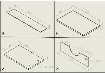
view of the coil holder. ... 35 Figure 2.9- Isometric view of the coil housing parts. (a) Bottom panel. (b) Side panel. (c) Top
panel. (d) Front panel. Dimensions given in mm. ... 35 Figure 2.10- 3D model of the cable support. (a) Isometric view of the cable support for the
Figure 2.11- Side fixing system. Dimensions given in mm. ... 36
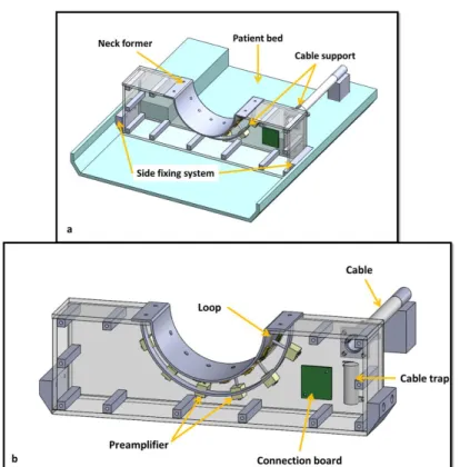
Figure 2.12- Illustration of coil assembly. (a) 3D model of the coil holder and electronics mounted on the patient table. (b) Detailed view of neck coil including housing and electronics. ... 37
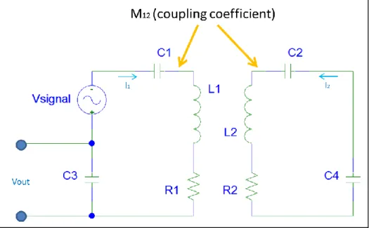
Figure 2.13 - Illustration of the elliptical loop and the equivalent lumped element model. ... 38
Figure 2.14– Screen caption impedance approximation using ADS. ... 38
Figure 2.15- Impedance of the elliptical loop. (a) Loaded coil. (b) Unloaded coil. ... 39
Figure 2.16- PSPICE circuit model for tuning frequency. ... 39
Figure 2.17- Transmission line terminated with a load impedance. Source : Pozar, 2009 ... 40
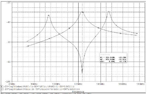
Figure 2.18- PSPICE screen shot of S21 measurement for the tuning frequency. ... 41
Figure 2.19- ADS model of tuning circuit. ... 41
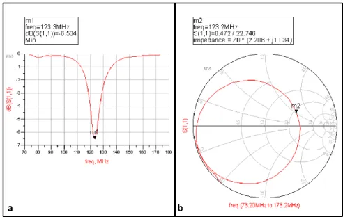
Figure 2.20- ADS screen shot of frequency response. (a) S11 linear plot. (b) S11 polar plot. ... 42
Figure 2.21- Block diagram illustrating impedance matching. ... 42
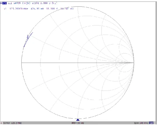
Figure 2.22- Coaxial cable S11 measurement for center frequency - 123.2MHz, span-100MHz. . 44
Figure 2.23- Lumped matching network for Zcoil inside the 1+jX circle of the impedance Smith chart. Source : (Pozar, 2009) ... 44
Figure 2.24- Coil with impedance matching network. ... 45
Figure 2.25- ADS model of tuning and matching circuits. ... 45
Figure 2.26- ADS screen shot for frequency response of the matching circuit. ... 46
Figure 2.27- Active detuning circuit. ... 46
Figure 2.28- PSPICE model of active detuning circuit. ... 47
Figure 2.29- PSPICE screen shot of S21 measurement of active detuning response. ... 48
Figure 2.30- Illustration of inductive coupling between neighboring loops. ... 49
Figure 2.31- Critical overlapping for reducing the mutual inductance. (a) Circular loops configuration. (b) Square loops configuration. Source : (Roemer et al., 1990) ... 50
Figure 2.32- Illustration of inductive coupling. ... 50
Figure 2.33- Preamplifier decoupling - impedance matching. ... 51
Figure 2.34- PSPICE model of preamplifier decoupling circuit. ... 52
Figure 2.35- PSPICE screen shot of S21 measurement for preamplifier decoupling. ... 52
Figure 2.36- PCB design. (a) The PCB used for matching and active detuning circuit. (b) Preamplifier socket board. ... 53
Figure 2.37- PCB design for the connection board. ... 54
Figure 2.38- Schematics of the patient table with the plug disposition. ... 54
Figure 2.39- Double loop probes. (a) 30mm. (b) 15mm. ... 57
Figure 2.40- Custom built calibration kit. O - open termination. S - short termination. L - 50Ω load termination. ... 58
Figure 2.41- Experimental setup: test rig, double loop probe, network analyzer. ... 59
Figure 2.42– Active detuning procedure using double loop probe (all elements detuned) ... 61
Figure 3.1- B1 field sensitivity profile simulations for one loop (a), two loops (b), four loops (c) and six loops (d). ... 66
Figure 3.2- B1 field sensitivity profile for Z=50mm. ... 67
Figure 3.3- Relative SNR simulations for one loop (a), two loops (b), four loops (c) and six loops (d). ... 67
Figure 3.4- Relative SNR for Z=50mm. ... 68
Figure 3.5- MATLAB script validation ... 68
Figure 3.6- Magnetic field intensity profile for a single rectangular loop. ... 69
Figure 3.7- Frequency response for a single rectangular loop. ... 70
Figure 3.8- Magnetic field intensity profile for a two rectangular loops array. ... 70
Figure 3.9- Frequency response for a two rectangular loops array. ... 71
Figure 3.11- Magnetic field intensity profile for a four rectangular loops array. ... 72
Figure 3.12- Frequency response for a four rectangular loops array. ... 72
Figure 3.13- Frequency response of decoupling for a four rectangular loops array. ... 73
Figure 3.14- Magnetic field intensity profile for a six rectangular loops array. ... 73
Figure 3.15- Frequency response for a six rectangular loops array. ... 74
Figure 3.16- Frequency response of decoupling for a six rectangular loops array. ... 74
Figure 3.17- Top view of the coil assembly. ... 75
Figure 3.18- Zoomed view of the coil electronics. ... 75
Figure 3.19- Resonant frequency of channel 1. ... 76
Figure 3.20- Resonant frequency of channel 2. ... 77
Figure 3.21- Resonant frequency of channel 3. ... 77
Figure 3.22- Resonant frequency of channel 4. ... 78
Figure 3.23- Resonant frequency of channel 5. ... 78
Figure 3.24- Resonant frequency of channel 6. ... 79
Figure 3.25- Q ratio. (a) Loaded. (b) Unloaded. ... 80
Figure 3.26- Active detuning of channel 1 - 54.03dB. ... 81
Figure 3.27- Active detuning of channel 2 - 47.31dB. ... 81
Figure 3.28- Active detuning of channel 3 - 44.69dB. ... 82
Figure 3.29- Active detuning of channel 4 - 41.89dB. ... 82
Figure 3.30- Active detuning of channel 5 - 40.28dB. ... 83
Figure 3.31- Active detuning of channel 6 - 46.79dB. ... 83
Figure 3.32- Inductive decoupling between CH 1-2. ... 84
Figure 3.33- Inductive decoupling between CH 2-3. ... 85
Figure 3.35- Inductive decoupling between CH 4-5. ... 86
Figure 3.36- Inductive decoupling between CH 5-6. ... 86
Figure 3.37- Preamplifier decoupling of channel 1 - 45.9dB. ... 87
Figure 3.38- Preamplifier decoupling of channel 2 - 33.71dB. ... 88
Figure 3.39- Preamplifier decoupling of channel 3 - 27.3dB. ... 88
Figure 3.40- Preamplifier decoupling of channel 4 - 39.97dB. ... 89
Figure 3.41- Preamplifier decoupling of channel 5 - 38.02dB. ... 89
Figure 3.42- Preamplifier decoupling of channel 6 - 35.47dB. ... 90
Figure 3.43- SNR maps of the water phantom obtained using the custom-built coil (a) and the commercial coil (b). ... 91
Figure 3.44- Noise covariance matrix. ... 92
Figure 3.45- SNR map of the human subject phantom obtained using the custom-built coil (a) and the commercial coil (b). ... 92
Figure 3.46- FLASH image of the spinal cord obtained using the custom built coil with acceleration 2. ... 93
Figure 3.47- FLASH image of the spinal cord obtained using the commercial coil with acceleration 2. ... 93
Figure 3.48- FLASH image of the spinal cord obtained using the custom built coil with acceleration 3. ... 94
Figure 3.49- FLASH image of the spinal cord obtained using the commercial coil with acceleration 3. ... 94
LIST OF SYMBOLS AND ABBREVIATIONS
The list of symbols and abbreviations presents the symbols and abbreviations used in the thesis or dissertation in alphabetical order, along with their meanings.
EPI Echo-Planar Imaging FOV Field-of-view
GE General Electric
GRAPPA GeneRalized Auto-calibrating Partially Parallel Acquisition
MR Magnetic resonance
MRI Magnetic resonance imaging MRS Magnetic resonance spectoscropy
NF Noise figure
NMR Nuclear magnetic resonance
PILS Partially parallel Imaging with Localized Sensitivities PLA Polylactide RF Radio frequency RL Return loss ROI Region-of-interest Rx Receive SE Spin Echo
SENSE SENSitivity Encoding
SMASH SiMultaneous Acquisition of Spatial Harmonics SNR Signal-to-noise ratio T1 Longitudinal relaxation T2 Transverse relaxation TE Echo time TR Repetition time Tx Transmit Tx/Rx Transmit/Receive
CHAPTER 1
INTRODUCTION
The technology of magnetic resonance imaging (MRI) is based on the development of the unified theory of magnetism by James Clerk Maxwell in the 1960s. This discovery demonstrated that electromagnetic waves can penetrate matter and empty space. The physicists Felix Bloch and Edward Purcell discovered the nuclear magnetic resonance phenomenon in 1945, a discovery which led to winning the Nobel Prize in Physics in 1952 (Sherrow, 2007). The magnetic field applied to the human body induces resonance of the hydrogen atoms due to radio energy. Hydrogen is one of the most common elements of the human body, being present in various amounts in body cells and tissues. In 1970, MRI was first used as a medical diagnostic tool by Raymond Damadian, a medical doctor and research scientist. In 1972, Paul Lauterbur acquired the first MRI image and Damadian patented the first MRI machine (Damadian, 1972).
MRI has the advantage of not using ionizing radiation, while having a good spatial resolution. The imaging can be acquired in every direction or section with a high contrast, which offers a good distinction between the tissues. The information provided is specific to physiology such as vascularization, temperature, cardiac function. The disadvantages are the long acquisition time, the low signal-to-noise ratio (SNR) level, and the movement artifacts. Moreover, claustrophobia encountered by some patients can be mentioned as one of the limitations (Cohen-Adad, 2014).
1.1 MRI technology review
1.1.1 Basic principle
MRI is based on the nuclear magnetic resonance (NMR) phenomenon of atom nuclei, most commonly the hydrogen atoms (H1) which are present in the tissue that needs to be imaged. The hydrogen atom has a nucleus with a single proton and an electron orbiting the nucleus. The proton has an intrinsic propriety called spin, which means that it rotates around its axis. Due to the combination of spin and electric charge, the proton is characterized by an angular momentum and a magnetic moment. The magnetic moment makes the proton behave like a small magnet, being affected by electromagnetic waves and external magnetic fields.
When an external magnetic field, B0, is applied the spins align along the direction of the magnetic field lines (z-axis). In addition, the spins begin to wobble around their axis also known as
precession. The precession frequency is called Larmor frequency and is proportional to the applied magnetic field strength. The Larmor frequency is given by the following equation:
𝜔0 = 𝛾0∙ 𝐵0 (1.1)
Where 𝜔0 is the Larmor frequency [MHz], 𝛾0 is the gyromagnetic ratio particular to the nucleus ( 𝛾𝐻1 = 42.58 𝑀𝐻𝑧/𝑇), 𝐵0 is the magnetic field strength [T].
One can excite the spins that precess around 𝐵0 by sending an electromagnetic wave using an RF coil at the Larmor frequency, also known as the resonance condition. The spins will be tipped from the z-axis to the transverse plane, resulting in a net magnetization in the transverse plane. After the RF waves are turned off, the spins will tend to come back to the initial state (relaxation), thus emitting RF waves or MR signal (Weishaupt, Kochli, & Marincek, 2006). Two types of relaxation of the protons occur: longitudinal relaxation (T1) and transverse relaxation (T2). Figure 1.1 illustrates the MRI principle. Differences in hydrogen protons binding with the surrounding molecules result in T1 and T2 relaxation times significantly different between tissues.
Figure 1.1- Illustration of magnetic resonance imaging principles.
(a) Spins rotate in random directions without any external magnetic field. (b) Spins align along the B0 field inducing a longitudinal magnetization Mz and rotate at the Larmor frequency (e.g. 127 MHz for 3T). (c) An RF wave of 90 ° is applied, which has the effect of (d) phasing the spins
of the proton and inducing transverse magnetization Mxy which precesses at the Larmor frequency. When the RF wave stops, the spins of protons will regain their stability by two relaxation processes (e) longitudinal relaxation, when the spins realign themselves to the field B0
and which is characterized by the relaxation time T1, and (f) the transverse relaxation, that corresponds to the phase shift of the spins in the XY plane and which is characterized by the time
1.1.2 MRI system architecture
Figure 1.2- MRI system architecture. Source: (Prince & Links, 2006) The main components of an MRI system are (Prince & Links, 2006):
- Main magnet – The magnet provides high stability field strength. Typical field strength in clinical scanners as of 2015 is 1.5T (~63MHz for 1H protons) or 3T (~125MHz for 1H protons). The generated magnetic field is known as the B0 field. The most important characteristic of the main magnet is the homogeneous field distribution within the center of the magnet (bore) with a tolerance of ±5 𝑝𝑝𝑚. The homogeneity of the field is controlled through the process of shimming which uses shim coils to correct the field distribution when necessary. Depending on the method of field generation a series of magnets can be distinguished: resistive magnets, permanent magnets and superconducting magnets (Prince & Links, 2006).
- Gradient coils – The gradient coils are notably used for slice selection and spatial encoding. The gradient coils alter the B0 field along the x, y, z axes by adding or subtracting magnetic fields. This added magnetic field varies linearly as a function of distance along a given axis. Gradient coils are usually characterized by the maximum gradient strength [mT/m], rise time – time to maximum gradient amplitude and slew rate
– maximum gradient amplitude/rise time (Weishaupt et al., 2006). Note that gradient coils can also be used to encode water diffusion in diffusion-weighted imaging (Hagmann et al., 2006).
- RF coils – These coils are used for transmitting and/or receiving RF waves at (or close to) the Larmor frequency. They are categorized as transmit coils (Tx), receive coils (Rx) or transmit-receive coils (Tx/Rx). In addition, depending on the covered area the RF coils can be divided in volume coils and surface coils. The RF excitation is produced using the transmit coil usually applied over the entire volume using volume coils. The magnetic field produced by the RF coil is defined as B1 field. The magnetic field generated by the transmit coils is noted B1+ , while the receive coil generates B1- field. In the reception part of the magnetic resonance (MR) signal, the SNR has to be improved. The disadvantage of the volume coils is that they pick up more noise resulting in a SNR decrease. Therefore, surface coils are preferred in the receive mode due to the closer positioning with respect to the region-of-interest (ROI). The interactions between the transmit coil and the receive coil have to be limited due to the fact that both coils are tuned to the same frequency, otherwise the B0 field profile can be altered.
- Shim coils – These coils are used to ensure homogeneous B0 field within the region of interest through a procedure called “active shimming”.
- Electronic systems for controlling the transmission and reception of RF signals – These systems consist of gradient amplifiers, RF electronics including receivers and transmitter control units, the pulse sequence computer and image reconstruction computer.
- Control console – Used for manipulating and controlling the system by the MRI operator. For example, the Siemens console is called “Syngo”.
1.1.3 MRI acquisition
We distinguish two types of MR applications: (i) MR imaging (MRI), which consists of obtaining a detailed representation of the anatomy and (ii) MR spectroscopy (MRS), which consists of obtaining information about metabolic content within a specified ROI.
The spatial encoding and acquisition of an MR signal is achieved using gradient coils and RF coils, respectively. Let’s look at an example of acquisition in the axial plane using a Spin Echo (SE) sequence. Firstly, the slice selection is made using a magnetic gradient along the z-axis. As it was mentioned before the magnetic field lines are oriented along the z-axis. Due to the change in the resultant magnetic field, the Larmor frequencies linearly changes along the z-axis. Therefore each slice perpendicular to the z axis will have its unique frequency. Moreover, if the frequency of the RF pulse excites only the protons within the desired slice, the other slices remain unaffected. The thickness of the slice is determined by the strength of the gradient and the bandwidth of the RF pulse. A thin slice is characterized by a strong gradient and a thick slice by a weak gradient. The position of the slice can be changed by changing the central frequency of the RF pulse (Weishaupt et al., 2006).
For MRI, after the slice has been selected, it has to be spatially encoded in order to obtain an image. The spatial encoding consists of two phases: phase encoding and frequency encoding. The spatial encoding is achieved by using additional gradients for x and y axis. The phase encoding is realized by applying a magnetic gradient along the y axis. The applied gradient will cause a phase shift linearly as a function of position along the y axis. The amplitude and duration of the phase encoding gradient will determine the resultant phase shift. Each line along the y axis will have a unique phase. The second stage of the spatial encoding is realized using the frequency encoding gradient. If the magnetic gradient is applied along the x axis, it will result in a change of Larmor frequencies along the axis. The received MR signal is a frequency spectrum. Each unique frequency will correspond to a column of the slice. Consequently, using the phase and frequency information for every point in the slice one can spatially localize every volume element also known as voxel (Weishaupt et al., 2006).
The temporal delay between repeated measurements is called repetition time (TR). The image quality depends also on the phase-encoding gradient. The acquisition time for SE sequences varies depending on repetition time, phase encoding steps, and number of averages. (Schoenberg, Dietrich, & Reiser, 2007).
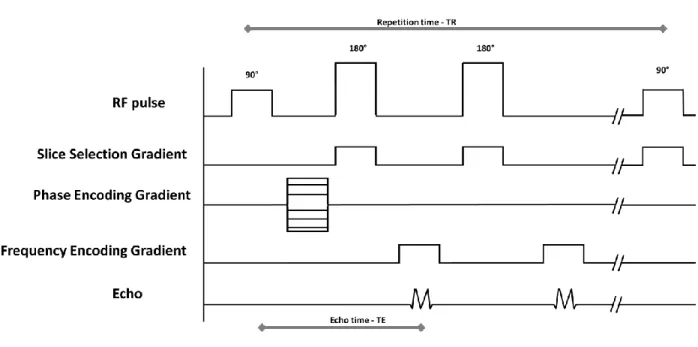
Figure 1.3- Illustration of simplified pulse sequence. Inspired from (Ballinger, 1996) The MRI raw data is stored in a matrix also called “k-space”, which represents the frequency distribution of the MRI data. The center of the k-space corresponds to low frequencies (contrast of the image) while the edge of the k-space corresponds to high frequencies (spatial resolution of the image). The image can be obtained by applying a 2D Fourier transform.
A basic pulse sequence including RF excitation, phase encoding and the frequency encoding of the slice is illustrated in Figure 1.3 .The amount of time between two consecutive RF excitation pulses is called repetition time (TR). Moreover, the echo time (TE) is defined as the time between the RF excitation pulse and the MRI signal sampling.
1.1.4 Parallel imaging
One limitation of the traditional pulse sequence is the acquisition time. A solution to reduce acquisition time is to use parallel imaging techniques.
Parallel imaging takes advantage of high density surface coil arrays. Since the acquisition time is dependent to the acquired number of phase-encoded echoes, it can be reduced if the k-space is under-sampled. A common problem in image reconstruction process is the aliasing. Aliasing is a common MRI artifact which occurs when the FOV is smaller than the imaged body part. In case of aliasing, the body part being imaged which is located outside the FOV will be project to the
other side of the image. A solution is to use the sensitivity profiles of the coils to mathematically reconstruct the image and remove aliasing. Consequently, the coil performance regarding the coil acceleration is related to the coil geometry also called the g-factor. From the parallel acquisition perspective, a lower factor offers better coil performances. The lowest factor is 1. A high g-factor is associated with reconstruction artifacts and lower SNR. Another characteristic of the parallel imaging techniques is the acceleration factor which is represented by the number of lines that are under-sampled with respect to the k-space.
A series of reconstruction methods that use the spatial information provided by the sensitivity profile of the receive coil array to substitute part of the phase encoding generated by the magnetic field gradients have been proposed. They include: SiMultaneous Acquisition of Spatial Harmonics (SMASH) (Sodickson & Manning, 1997), SENSitivity Encoding (SENSE) (Pruessmann, Weiger, Scheidegger, & Boesiger, 1999), Partially parallel Imaging with Localized Sensitivities (PILS) (Griswold, Jakob, Nittka, Goldfarb, & Haase, 2000) and GeneRalized Auto-calibrating Partially Parallel Acquisition (GRAPPA) (Griswold et al., 2002).
1.2 Rationale
The RF coil is an important component of the MRI system. It is used to transmit and receive MRI signal. The coil design has to be properly adapted to the ROI that needs to be imaged and the desired imaging protocol. Therefore, mechanical aspects such as coil element dimension and positioning or electronic aspects such as electronic component performances have an important impact on the coil performance (Keil, 2013).
The current thesis is focused on developing a RF coil for imaging the human cervical spinal cord. The spinal cord is an important component of the central nervous system and it occupies the upper two-thirds of the vertebral column (Gray, Goss, & Alvarado, 1973). The spinal cord assures the transmission of neural signal from the brain to the rest of the body, being responsible for three important functions: body sensation, automatic and motor control. These functions can be compromised (e.g., paralysis) in pathologies such as traumatic spinal cord injury, multiple sclerosis or cancer. This brings the rationale for imaging the spinal cord non-invasively with MRI. Having a coil that provides high SNR and low g-factor will enable higher spatial resolution and acceleration factors, which will in turn improve diagnosis.
1.3 Research objectives
The main objective was to design and construct a highly sensitive coil for proton imaging of the human cervical spinal cord at 3 Tesla (Larmor frequency: 123.2 MHz). The principal objective can be divided into specific objectives:
To develop an electromagnetic simulation framework for the assessment of the magnetic field sensitivity profile for comparing different coil array geometries in order to determine the optimal configuration;
To design and construct a receive-only coil including ergonomic support of the neck compatible with the Siemens Trio scanner infrastructure available at our research center; To evaluate the performance of the RF coil array at the bench using a water phantom;
security recommendations will also be evaluated;
1.4 Literature review
1.4.1 RF coils
1.4.1.1 Phased array coils
The design of high-density surface RF coils is an important research subject for many groups around the world since the beginning of the 1990s. The current literature review will be focused on a series of important aspects that have to be taken into consideration by the coil designer such as theoretical modelling of SNR, electromagnetic simulations of the sensitivity profile of the RF coil and finishing with different implementations of multi-channel phased arrays.
One of the most important principles used in the development of receive coils is the reciprocity theorem. This theorem which was initially formulated in antenna theory is stating that the characteristics of an antenna in the receiving mode can be obtained from the same antenna used in the transmitting mode (Neiman, 1943). Hoult and his associates (D.I Hoult & Richards, 1976) demonstrated that the magnetic field produced at a point in space by a unit current in a RF coil is proportional to the electromotive force induced in the coil by a magnetic dipole at the same point. Another research based on a series of bench experiments has provided the mathematical basis to derive the equations for the B1 field generated by the RF coils. The purpose of knowing the field sensitivity profile is to correctly approximate the received signal in an NMR experiment (D. I. Hoult, 2000). Another group developed the reciprocity theorem for NMR which states that the sensitivity of NMR signal from a sample is proportional to the intensity of the magnetic field generated by the current circulation in the coil (D. I. Hoult & Richards, 2011). The experiment of Ackerman demonstrated that SNR can be improved by a surface coil close to the ROI of the sample (Ackerman, Grove, Wong, Gadian, & Radda, 1980). Consequently, SNR is influenced by the magnetic field intensity received by the coil. The key parameters for defining the quality of a MRI acquisition are the SNR and the acquisition time. The time of acquisition of a MRI image dataset can be reduced either by using faster gradients or by optimizing the receiving RF technique. The initial proposed optimization of the RF coil consisted of connecting multiple coils to form an array structure. The acquisition time decreased due to better spatial localization of the MRI signal.
To begin with, an initial optimization of the RF coils was the introduction of phased-arrays (Roemer, Edelstein, Hayes, Souza, & Mueller, 1990). Since then, the development of new arrays has pushed forward with an increased number of channels improving the sensitivity of the scanners. The advantages of having an array of coils are the increase of SNR and increased field-of-view (FOV) comparable with body imaging. In addition, the required scan time is reduced due to the number of channels and the optimized method of phase encoding. The approach used by Roemer et al. to optimize the SNR in a 3D volume consisted of comparing three different surface coil configurations: an 8-cm square coil, a single large 30x15-cm rectangular coil and a four element phased array made of 8-cm square coils. The computed SNR for the 4-channel linear spine array provided a SNR 2 to 3 times higher than a single channel rectangular coil for the same FOV at the same level of depth. Moreover, in the case of circular loop coils, the optimal SNR was achieved at a depth equal to diameter of the coil. High resolution spin-echo images of the thoracic and lumbar spine were acquired to demonstrate the phased array imaging viability. Another aspect discussed in the article was the problem of interactions among neighboring coils which can be limited by overlapping adjacent coil in order to reduce mutual inductance or by using low impedance preamplifiers decoupling technique. The distance between the centers of two co-planar circular loops for cancelling their mutual inductance was found to be 0.75 times their diameter, compared to 0.9 times for square coils. In addition, the authors proposed various image reconstruction techniques for determining weights for combining images or spectroscopic data such as sum-of-squares combination.
Using the framework developed by Roemer, in 1991 Hayes et al. (Hayes, Hattes, & Roemer, 1991) built a volume 4-channel phased array having two coils placed anterior and two coils posterior to the human pelvis. An SNR improvement of 80% was obtained for a single image using the array when compared with the body coil. Additional comparisons with two-channel phased array and a Helmholtz pair revealed similar results. Thus, the SNR improvement can be used to reduce the slice thickness and to reduce the number of excitations. Future research (Hayes, Dietz, King, & Ehman, 1992) was focused on the quantitative assessment of SNR in pelvic imaging conducted on water-filled phantom that simulated RF loading effects. The SNR produced by the longitudinal array was 2.3 to 3.1 times higher than the SNR offered by the body coil.
Depending on the ROI, a custom built RF coil can provide better performances than the commercial body arrays. For example, a two and four channel phased arrays for 1.5T General Electric (GE) scanner have been proposed by Wald (Wald et al., 1995) to increase the sensitivity and resolution of human brain cortex imaging. The main motivation for developing phased arrays is the lack of signal intensity uniformity over a larger area such as the human brain. The sensitivity of the coils at the surface of the cortex was 600% higher than the commercial head coil. In addition, the signal decrease with the depth which is characteristic to the size of the component coils can be problematic when an optimal view of different regions of the image is required. A solution to this problem is low pass filtering of the anatomical image by a phantom image. For SNR measurements, the method is similar to the one proposed by Hayes (Hayes et al., 1991) and implies the acquisition of two successive images of the phantom. The resultant SNR was calculated by the sum of the two images and the noise at the same given pixel in the image. Another application of the phased arrays was a prototype cardiac 4-channel phased array receiver coil for 1.5T GE Sigma scanner. The array comprised of a 2-channel cylindrical array positioned on the chest and a separate 2-channel planar array positioned at the back (Constantinides, Westgate, O'Dell, Zerhouni, & McVeigh, 1995). The computed SNR over the heart region was 1.1 to 2.85 times higher than a commercial flexible coil. Another phased array developped on a 1.5T GE scanner for the assessment of atherosclerotic plaques in the carotid artery was implemented for obtaining high resolution images (Hayes, Mathis, & Yuan, 1996). The 2-channel silver-braid carotid phased array provided improved FOV, an enhanced adaptability to wide variations in patient anatomy and reduced susceptibility to motion artifacts better than the single channel circular commercial coil. The maximum array improvement compared to the 3-inch commercial coil was 37 %. The SNR of the image acquired with the carotid phased array was 93, being higher than the SNR of 80 generated by the commercial coil.
1.4.1.2 Simulations
A large number of research groups have focused their studies on developing an approach to numerically model the ultimate SNR. A series of experiments conducted on different body coil combinations at different intensities of the static magnetic field revealed that the intrinsic SNR is proportional to the B0 field (Edelstein, Glover, Hardy, & Redington, 1986). The conventional approach to measure the SNR uses line integrals over the electric currents in the coils. A novel
method based on surface integrals over magnetic dipoles which cover the area enclosed by the coil offered newer perspectives (Jianmin, Reykowski, & Dickas, 1995). This method was used to derive the maximum SNR for an ideal receive array coil. The calculated SNR of the array was 35.8% higher than for single circular loop size-optimized and linearly polarized coil. When the sample noise is dominant, the intrinsic SNR for gradient-encoded imaging can be improved by minimizing the power deposition in the sample while maintaining a proper circularly polarized magnetic field at the ROI (Ocali & Atalar, 1998). The electromagnetic field optimization and intrinsic SNR maps obtained from simulations were compared to phantom image acquisitions. The results showed that overall performance can be improved if the electromagnetic field is focused on the ROI to compensate the skin effect which produces signal loss.
More electromagnetic field considerations related to the optimal intrinsic SNR were made by Ohliger et al. (Michael A Ohliger, Grant, & Sodickson, 2003). Their aim was to optimize the spatial encoding proprieties of the RF coil sensitivity profile instead of changing the geometry of the conductors. They proposed a protocol for obtaining an optimal coil sensitivity profile using plane waves simulations over an elliptic phantom for a given acceleration. The disadvantage of using higher accelerations for increased field strengths was the drop in SNR. The results show considerable advantages in terms of acceleration for high static magnetic field strengths when using 2D under-sampling of k-space. Another useful insight was the impact of the electrical conductivity of the sample on the use of surface coils for spatial encoding. The optimum achievable SNR profile was higher on the edges of the sample and lower in the center of it for 1.5T and 5T static field strengths.
Using a different approach, an important paper (Wright & Wald, 1997) is focused on the optimization of SNR of the receive coil by taking into account the efficiency of the phased array transmit coil. The benefit of using this approach is that the developed theory can be used also for developping transmit array coils. Using numerical simulations, multiple geometries of planar arrays of 2x2, 4x4 and 8x8 elements were compared to a single coil with similar size. Results show that the sensitivity profile is improved in the region near the array coil. In order to optimize the ratio of transmitted power, one can optimize the SNR in the receiver case and use the resultant weighting coefficients based on the reciprocity theorem.
The acceleration limit and its relation with the SNR was studied by Wiesinger et al. (Wiesinger, Boesiger, & Pruessmann, 2004). From SENSE parallel sensitivity encoding it is known that the SNR is inversely proportional to the geometry factor. One of the limitations of the SNR model is that it cannot be used for in vivo applications. The results show that the SNR performance was almost optimal when using low to moderate acceleration of geometry factors near 1. For higher acceleration, the exponential increase of the geometric factor decreased the achieved SNR. The behavior of the critical reduction factor was different depending on near and far field regimes. The critical reduction factor is independent of the static magnetic field and object size in the near field regime. In the case of far field, the factor is dependent on the object size and the B0. For B0 field higher than 7T the far field regime could be used for parallel imaging.
Furthermore, the same author proposes a method for approaching the ultimate SNR using finite coil arrays (F. Wiesinger, 2005). In order to evaluate the parallel imaging performance of finite arrays, the circular current distributions and theoretical SNR were compared. To render the calculations more realistic, coil sensitivity profile and noise receiver noise were taken into account in the SNR computations. The electrodynamic dependencies of SNR were the static field strength and the sensitivity profile of the coils. Multiple coil arrangements with various elements distributed around a spherical object which approximates the human head were compared. For the case of a static field of 1.5T, the configuration with 32 coils offered 4.6 times higher SNR than the 8 coil configuration.
Having a powerful tool for the electromagnetic simulations can help the developer to achieve the best coil configuration for its application. Full-wave numerical MoM analyses for evaluating the intrinsic SNR were purposed (Kumar & Bottomley, 2006; Kumar, Edelstein, & Bottomley, 2009). The experiments conducted using a circular loop coil configuration revealed that the noise related to the loop increases relative to the sample noise when the loop radius decreases. The noise figure (NF) of a 3cm diameter coil for a 3T static field was 0.8dB compared to 0.2dB for a 7T static field. In addition, strip detectors with length about 1.3 (+/- 0.2) times the depth of interest offered comparable results to loop coils with similar dimensions, the only difference was the characteristically different spatial distribution of the field from a loop.
1.4.1.3 Coil design
The parallelization of the receiver proved to enhance the SNR with the increased number of coil elements when compared to volume coils or single coils with the same covering area. In order to achieve the optimum SNR, the configuration of the coil array is important. Multiple papers focused on the coil design illustrate different approaches depending on the application. The next section will be focusing on the coil design for surface arrays. Depending on the region of interest and the desired scanning protocol, the designer has to decide the number of channel used in a receive phased array.
An article focused on the general design considerations of coil arrays for parallel MRI made a qualitative analysis from the theoretical and the practical point of view (Michael A. Ohliger & Sodickson, 2006). The qualitative analysis made on the spatial encoding using coil arrays offered a model for the emulation of the spatial harmonics and a solution for unfolding the aliased data. The numerical models were developed using SENSE and SMASH image reconstruction techniques. Depending on the particular image plane orientation, FOV and acceleration factor, the coil design has to be optimized in order to achieve the maximum SNR. For the cervical region, the authors suggest using an adaptive combination of coil array elements due to the degree of freedom in imaging multiple anatomical regions with the same coil array.
Another paper addresses the problem of maximum number of elements that is required to achieve high quality images and reduced acquisition time (Fujita, 2007). The emphasis on preamplifiers is made due to the fact that they play an important role beyond signal amplification. The preamplifiers are used for achieving the optimal SNR and to improve the performance of parallel imaging techniques in terms of proper decoupling between coil array elements. Important considerations have to be taken into account when designing the coil array to properly balance the spatial resolution (SNR) and the temporal resolution or the speed of acquisition for the desired clinical application.
In order to achieve a greater degree of flexibility of the coil design, a modular design of receive only arrays was proposed (De Zanche, Massner, Leussler, & Pruessmann, 2008). The difference of this approach is that the preamplifier board, matching and active detuning circuits are built in a circuit board for each coil. This type of configuration offers robustness to geometrical variations of coil loop arrangements being able to achieve reconfigurable coil arrays. The results illustrated
that the independent distribution of coils without overlap provides a reduced noise correlation between elements over the configuration with overlapped coils.
A 32-channel 3T receive-only phased-array head coil was developed for human brain imaging compatible with SENSE reconstruction technique (Wiggins et al., 2006). The coil elements were arranged in a helmet shaped having a soccer ball pattern of hexagonal and pentagonal symmetry. The quantitative evaluation of the SNR showed a 3.5 times improvement in the cortex compared to the 8-channel head coil. The array was able to achieve acceleration of four and five while providing high resolution brain images. Moreover, the coil array offered reduced g-factors for x and y accelerations.
In addition, a size optimized for five age groups for pediatric brain imagining consisting of 32 channels tight fitted to the former was proposed (Keil, Alagappan, et al., 2011). The coil-former was designed using 3D MRI images for each group. The commercial coil used for brain imaging of infants is a birdcage coil. The highest SNR increase was observed in the neonate coil with up to 3.6 more within the brain cortex compared to the 32-channel coil for adults. The conclusion of the study was that the size and the fitting of the coil around the ROI is very important making possible sensitivity gains for accelerated brain imaging in infants.
The previously presented 32-channel coil for adults was compared with a 64-channel 3T receive-only coil placed in a similar holder (Keil et al., 2013). The split-former design of the holder makes the coil very ergonomic for the patient being suitable for every-day clinical use. The unaccelerated images offered 1.3 times more signal in the brain cortex for the 64-channel array. An acceleration of 4 times was achieved using the new coil, while maintaining a low noise amplification compared to the previous coil.
The high parallelization of the receive arrays was analyzed and reviewed in a recent paper (Keil & Wald, 2013). The aim was to present the theoretical and practical aspects for developing high density arrays based on the information obtained from theoretical modelling and experiments of the ultimate SNR. In order to build highly parallel arrays, the interactions between neighboring elements have to be reduced, thus circuits for achieving the proper level of preamplifier decoupling, taking into account the fact that the coil impedance needs to be matched to the required noise figure matching of the preamplifier. The suggested initial phase of the construction of a RF coil consisted of the complete 3D design of the coil housing and electronics, including
the cable routing and preamplifier mounting supports. The mass production of elements and the population of the coil former with all elements was found to be impractical .It is recommended to add individual loops and to assess their performance before adding additional loops. The next neighboring elements optimization was found to be the most consuming coil procedure, a test rig being necessary in order to detune all the other elements. Current parallel imaging techniques use higher numbers of detectors driven by sensitivity arguments. The individual sensitivity profile of each coil is used for spatial information during signal encoding step.
1.4.2 Coils for spinal cord
Figure 1.4- Pictures of spine array coils for 3 T (top) and 7 T (bottom). Source: (Cohen-Adad & Wheeler-Kingshott, 2014)
The following sections will review different coil configuration proposed for imaging the spinal cord in humans.
A head/neck coil with 16 independent channels combined to clusters was proposed for Siemens scanners (Reykowski, Hemmerlein, & Fischer, 2005). The design offered improved g-factors in different directions such as anterior-posterior, left-right and head-feet. Due to the modular design
of the channel combination, the coil can be combined with other matrix coils for extending the coverage area. The head area was covered by 12 elements with independent preamplifiers combined into 3 modes combiners. The neck region has 2 elements posterior and 2 anterior. The signals are combined in 2 modes matrices.
An optimized 16-channel receive-only array for cervical spinal cord imaging was proposed for a 3T General Electric scanner (Bodurka, Ledden, & Bandettini, 2008). The coil had a 4x4 arrangement of elements fixed on a rigid curved former. The loops had an elliptical shape of 8x6cm copper trace printed on a flexible substrate. The spacing between adjacent columns was adjusted to a ratio of 30% to improve the axial g-factors. Each element had an active detuning circuit and a passive detuning one, with additional baluns to cancel the common mode currents. The coil was initially validated using gradient echo imaging for phantom. Further validations were performed for human subject imaging using fast spin echo sequence with flow compensation and fat suppression and single shot echo-planar imaging (EPI) with SENSE. The results illustrate that the coil offered a large coverage from the brain visual cortex as low as the tenth cervical segment. The high resolution SENSE EPI capabilities offer the possibility of further fMRI investigation of the spinal cord.
An 8-channel Tx/Rx phased array coil composed of surface loop coils with a dimension of 12cm x 12cm was developed for spine imaging at 7T (Kraff et al., 2009). The coil was validated on 3 subjects by using 3D-FLASH sequence with an isotropic resolution of 0.57mm. The high spatial resolution illustrated the longitudinal ligaments or the venous drainage through the vertebral bodies. The g-factor for head-feet direction was reported 2.7 with an extended FOV of 40cm. A high field application of the RF Tx/Rx coils for the spine imaging on a 7T GE scanner proposed using adjustable inductive decoupling between adjacent elements (Bing et al., 2010). Three Tx/Rx coils (12cm x 12cm with four channels, 12cm x 8cm with six channels and 12cm x 6cm with eight channels) were built and compared. The novelty was the adjustable inductive decoupling which offered -25dB decoupling between nonadjacent elements in different loading conditions. The four-channel array achieved g-factor of 2, 3 and 4 without important artifacts in the reconstructed image. The proposed coil was not fully optimized for the spinal cord imaging, therefore better shimming and the reduction of motion artifacts could provide better performances.
Another coil design was proposed for brain and cervical spinal cord imaging (Cohen-Adad, Mareyam, Keil, Polimeni, & Wald, 2011b). The 32-channel receive coil was optimized for a 3T Siemens scanner: 4 of the channel were used to image the neck region, 3 of them for the spine and the remaining were distributed in a soccer ball pattern to cover the brain. The temporal SNR obtained by the custom built coil was 2 times higher for the brain region and 1.8 times for the cervical spinal cord when compared to the commercial coil. In addition, the authors reported high resolution diffusion imaging of the spinal cord at 0.6x0.6x5 mm3 using GRAPPA reconstruction without noticeable distortion.
A custom coil built for 3T Head/Neck/C-spine imaging was integrated with the spine coil to offer a large coverage and better accelerations (Keil, Biber, et al., 2011). The coil had 60 channels distributed in a hexagonal and pentagonal pattern. The coils were combined using low noise converters for multiplexing two channels onto a single output. The coil performances were compared with a 20 channels and a 32 channels coils. The 64-channel coil provided an improved SNR in the cervical region of 1.8 times than the 20-channel head/neck array. The sensitivity profile was slightly improved when compared with the 32 channel brain coil, especially in the cortex.
A 4-channel coil array for ultrahigh field was prototyped and compared with a standard 3T coil (Sigmund et al., 2012). The 7T array had an improved SNR by a factor of 3.5 in the cervical region than the 3T coil. The increased SNR made possible depiction of internal structures such as the nerve roots and rostral-caudal blood vessels. The SNR and the magnetic field distribution provided by the coil were estimated using the Kellman method (Kellman & McVeigh, 2005). The cross-sectional areas of gray/white matter obtained using 7T images were similar to reports from histology.
An 1H MRS in the human spinal cord was developed and tested on healthy volunteers for a 7T field strength using RF shimming and travelling wave transmit approach (Anke Henning, 2012). The RF shimming was used due to the important susceptibility changes caused by the flow of cerebrospinal fluid and the respiratory motion of the patient. The transmit coil consisted of two radiative antennas fixed around the neck using a pillow filled with D2O. A custom built 30-channel sensitivity optimized array was used for signal reception. Inner volume saturation, VAPOR water suppression and 3rd order FASTERMAP shimming were applied to improve the
spectra. The final spectra for the C2/3 levels of the spinal cord had limited artifacts such as lipid contamination, ghosting, baseline or phase distortions.
Another dedicated cervical spinal cord with 4-channel transmit and 19-channel receive was implemented for 7T scanner (Zhao et al., 2014). The elements were placed on a close-fitting coil former. The transmission performances efficiency and absorption rate were evaluated using B1 field mapping and electromagnetic simulations. The SNR performances were compared with a 19 channels receive 3T neck array and 4-channel spine for 7T. The SNR was 4.2 times higher for the 7T array when compared to the 3T commercial coil. A higher acceleration was achieved using the 7T coil. Moreover, when compared to the 4-channel spine receive array for 7T, the SNR increased 1.5 times in the spinal cord. A spatial resolution of 0.3 mm was achieved in spinal cord imaging.
1.4.3 Synthesis of literature review
After reviewing the solutions proposed in the literature review, one can make some remarks and conclusions:
- There is a limited number of RF receive coils dedicated to the cervical region of the spinal cord, most of the available coils are covering the brain and the neck regions. These coils have a higher density for the brain, than for the neck region.
- The design of a RF receive-only coil has to be adapted to the anatomy to be imaged. Firstly, the coil former has to offer a high degree of comfort for the patient. Moreover, the distribution of the elements of the array has to be optimized in order to provide a large coverage, while producing uniform sensitivity profile.
- The recommended procedure for constructing an RF coil begins with electromagnetic simulations for determining the adequate loop geometry and alignment for the targeted area of imaging. Once the optimal configuration is found, one can start building the array using non-magnetic materials and low loss electronic components. Moreover, one can define the expected performance indicators for the bench measurements :
o Tuning frequency: Considering the magnetic field generated by the scanner for 3T is 123.2 MHz.
o Q factor ratio should be as high as possible; consequently the coil losses should have smaller in the power losses (Keil, 2013; Kyle M. Gilbert & Menon, 2015). o Active detuning: The amplitude difference between the maximum S21 when tuned
and the minimum S21 when detuned should to be less -35dB (Keil, 2013; Kyle M. Gilbert & Menon, 2015).
o Geometric decoupling: the decoupling level between neighboring loops should be less than -12dB (Keil, 2013; Kyle M. Gilbert & Menon, 2015).
o Preamplifier decoupling: The amplitude difference between the maximum S21 when the preamplifier is replaced by a conjugate impedance and the minimum S21 when the preamplifier is connected should be less than -15dB (Kyle M. Gilbert & Menon, 2015).
CHAPTER 2
MATERIALS AND METHODS
2.1 Electromagnetic simulations
The first step in the construction of the RF coil was the development of electromagnetic simulations of various configurations in order to determine the optimal element configuration in terms of loop geometry and positioning.
2.1.1 MATLAB
The electromagnetic simulations were developed for the assessment of the magnetic field sensitivity profile and the SNR maps. For the robustness of computation, the proposed numerical simulations are based on the Biot-Savart law. The numerical simulations consider quasistatic electromagnetic conditions, integrating the Biot-Savart law along the path of a loop circulated by a steady current. The quasi-static conditions use static assumptions for computing the magnetic flux density and the magnetic vector potential. The electric field is computed assuming a time-varying field. Using the electric field of the coil, one can approximate the losses generated in the sample. The simplified estimation neglects the mutual coupling between the elements, thus considering ideal preamplifier decoupling conditions and wavelength effects. The proposed model does not enforce all boundary conditions on the fields, while providing proper results for applications in MRI and MRS (Wright & Wald, 1997). The resultant B1 field for the combined array was determined using the sum-of-squares of individual field profiles of the elements.
2.1.1.1 Magnetic field sensitivity profile
The basis of the magnetostatics is a particular case of the Maxwell equations. The electric and magnetic fields can be generated and influenced by each other and by charges and currents (Lehner, 2008). The Maxwell equations for describing the magnetostatic conditions are listed below.
Table 2.1- Maxwell equations used in magnetostatics.
Name Differential form Integral form
Gauss’s law for magnetism ∇ ∙ 𝑩 = 0
∮ 𝑩 ∙ 𝑑𝑺 = 0 𝑆
Ampere’s law ∇ × 𝑯 = 𝑱
∮ 𝑯 ∙ 𝑑𝒍 = 𝐼𝐶 𝐶
Where ∇ is the divergence operator, B is the magnetic field density, the integral over a surface S with the surface element dS, H is the magnetic field intensity, J is the current density and the integral over a closed contour C with a segment element dl, Ic represents the current circulating through the loop.
Furthermore, one can establish a relation between B and H for vacuum conditions:
𝑩 = 𝜇0𝑯 (2.1)
Where 𝜇0 = 4𝜋 × 10−7𝐻/𝑚 representing the permeability of free space.
The objective of using the magnetostatic conditions is to characterize the magnetic field generated by different coil configurations. A formal method of calculating the magnetic field is using the vector potential A. Using the property that the divergence of the curl is equal to zero:
∇ ∙ (∇ × 𝒂) = 0 (2.2)
The Gauss’s law for magnetism in differential form can be written as:
𝐁 = ∇ × 𝑨 (2.3)
If the current density J(r) has a complete description then the magnetic vector potential can be determined from the current:
𝑨 = 𝜇0 4𝜋∫
𝑱(𝒓) 𝒓 𝑑
Where J(r) is the current density, r is the pointing vector from the coil to the observation point and the integral is over the whole volume of observation.
On the other hand, if we apply (2.3) to (2.4) we can write the Biot-Savart law. The Biot-Savart law describes the magnetic field generated by a steady current.
If one analyses the case of a small length element of wire, the resultant magnetic field is defined by: 𝑑𝑩 =𝜇0𝐼 4𝜋 𝑑𝒍 × 𝒓̂ 𝒓𝟐 (2.5)
Where I is the steady current, 𝜇0 is the permeability of the vacuum, 𝑑𝒍 is the length element of the wire, 𝒓̂ is the unit vector between the wire and the observation point.
Figure 2.1- Geometry of the magnetic field of a current circulating a small element of wire. Furthermore, the analysis of the magnetic field can be extended for a closed circular loop with the radius R. Figure 2.2 illustrates the magnetic field components (𝑑𝐵⃗⃗⃗⃗⃗⃗⃗ , 𝑑𝐵𝑥 ⃗⃗⃗⃗⃗⃗⃗ , 𝑑𝐵𝑦 ⃗⃗⃗⃗⃗⃗⃗ ) for a small wire 𝑧 element 𝑑𝑙 computed at the observation position defined by 𝑟 on the axis of the loop is the pointing vector between the wire and the observation point.
Figure 2.2- The magnetic field generated by a current loop segment on an arbitrary point on the center axis.
Using Biot-Savart law over a closed contour, it results:
𝑩 = ∫ 𝑑𝑩 =𝜇0𝐼 4𝜋∫
𝑑𝒍 × 𝒓̂ 𝒓𝟐
(2.6)
This integral can be approximated by the summation:
𝑩 ≈ 𝜇0𝐼
4𝜋∑
𝑑𝒍 × 𝒓̂ 𝒓𝟐
(2.7)
The approximation is valid when 𝑑𝒍 is small enough.
If we generalize the problem for a 3D Euclidian space, the components of 𝑑𝒍 and 𝒓̂ can be defined for each direction:
𝑑𝒍 = 𝑑𝑙𝑥𝒊̂ + 𝑑𝑙𝑦𝒋̂ + 𝑑𝑙𝑧𝒌̂ (2.8)
𝒓̂ = 1
𝑟[𝑟𝑥𝒊̂ + 𝑟𝑦𝒋̂ + 𝑟𝑧𝒌̂]
(2.9)
Where 𝑟 = √𝑟𝑥2+ 𝑟𝑦2+ 𝑟𝑧2.
𝑑𝒍 × 𝒓̂ = | 𝒊̂ 𝒋̂ 𝒌̂ 𝑑𝑙𝑥 𝑑𝑙𝑦 𝑑𝑙𝑧 𝑟𝑥 𝑟𝑦 𝑟𝑧 | = 1 𝑟[(𝑑𝑙𝑦𝑟𝑧− 𝑑𝑙𝑧𝑟𝑦)𝒊̂ + (𝑑𝑙𝑧𝑟𝑥− 𝑑𝑙𝑥𝑟𝑧)𝒋̂ + (𝑑𝑙𝑥𝑟𝑦− 𝑑𝑙𝑦𝑟𝑥)𝒌̂] (2.10) If we replace (2.10) in (2.7): 𝑩 ≈𝜇0𝐼 4𝜋∑ 𝑑𝒍 × 𝒓̂ 𝒓𝟐 = 𝜇0𝐼 4𝜋∑ 1 𝒓𝟑[(𝑑𝑙𝑦𝑟𝑧− 𝑑𝑙𝑧𝑟𝑦)𝒊̂ + (𝑑𝑙𝑧𝑟𝑥− 𝑑𝑙𝑥𝑟𝑧)𝒋̂ + (𝑑𝑙𝑥𝑟𝑦− 𝑑𝑙𝑦𝑟𝑥)𝒌̂] (2.11)
Since 𝑩 = 𝐵𝑥𝒊̂ + 𝐵𝑦𝒋̂ + 𝐵𝑧𝒌̂, the solution for each direction is :
𝐵𝑥 ≈𝜇0𝐼 4𝜋∑ 1 𝑟3(𝑑𝑙𝑦𝑟𝑧− 𝑑𝑙𝑧𝑟𝑦) = ∑ 𝑑𝐵𝑥 (2.12) 𝐵𝑦 ≈𝜇0𝐼 4𝜋 ∑ 1 𝑟3(𝑑𝑙𝑧𝑟𝑥− 𝑑𝑙𝑥𝑟𝑧) = ∑ 𝑑𝐵𝑦 (2.13) 𝐵𝑧 ≈ 𝜇0𝐼 4𝜋∑ 1 𝑟3(𝑑𝑙𝑥𝑟𝑦− 𝑑𝑙𝑦𝑟𝑥) = ∑ 𝑑𝐵𝑧 (2.14)
The magnitude of 𝑩 is given by:
|𝑩| = √𝐵𝑥2+ 𝐵𝑦2+ 𝐵𝑧2 (2.15)
2.1.1.2 SNR
The magnetic field sensitivity profile provides important information about the magnetic field distribution of the RF coil. For a quantitative evaluation of the RF coil, SNR simulations provide useful insights regarding the mutual noise between the elements of the array. The SNR was computed using the method proposed by Roemer (Roemer et al., 1990). Aiming to construct a uniform sensitivity image, the SNR can be calculated as:
𝑆𝑁𝑅 = √𝑩𝑻𝑹−𝟏𝑩∗ (2.16)
Since we have computed the magnetic vector potential and assuming a constant frequency, we can compute the mutual noise resistance matrix within a sample as (Roemer et al., 1990):
𝑹𝒊𝒌= 𝜔2𝜎 ∫ 𝑨
𝒊∙ 𝑨𝒋 𝑑3𝑉 (2.17)
Where Rik is the mutual noise resistance between coil i and coil k, ω is the angular frequency, σ is the conductivity of the sample, the magnetic vector potentials Ai of coil i, respectively Aj of coil j and the integral is computed over the volume V.
2.1.1.3 Proposed configurations
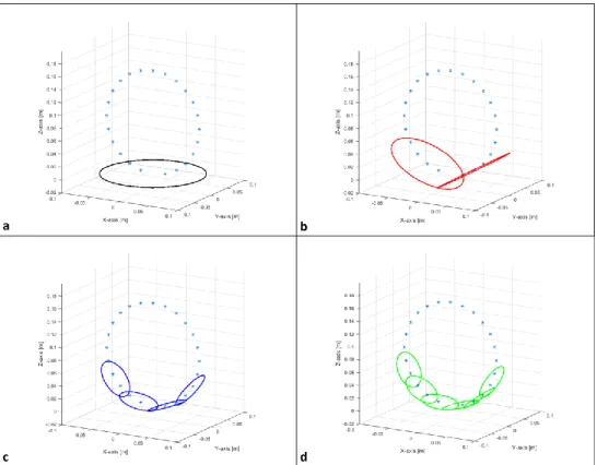
The simulations were run for 4 distinct configurations:
- Configuration a: single channel circular loop with 6cm radius - Configuration b: 2-channel array circular loop with 6cm radius - Configuration c: 4-channel array with circular loop with 3cm radius - Configuration d: 6-channel array with elliptical loop with 2.75cm x 3cm
These configurations were based on preliminary work, and account for the geometry of the neck. The elements were uniformly distributed in the lower half of 8cm cylinder. The radius of the cylinder is similar to the radius of the neck former (Figure 2.3). The suggested simulations are made in order to determine the optimal configuration for B1 field penetration and SNR.
Figure 2.3- Distribution of coils around the former (blue circle). (a) Single channel coil array. (b) 2-channel coil array. (c) 4-channel coil array. (d) 6-channel coil array.
The request for the B1 field sensitivity profile and the SNR maps were computed for space defined by:
- X axis – inferior limit: -20cm; superior limit: 20 cm; step size: 0.1cm; - Y axis – inferior limit: 0cm; superior limit: 0 cm; step size: 0.1cm; - Z axis – inferior limit: 0cm; superior limit: 40 cm; step size: 0.1cm.
2.1.2 FEKO
2.1.2.1 Validation of MATLAB simulations
We propose a validation of the scripts developed in Matlab using commercial software for electromagnetic simulations based on the Method of Moments (MoM) (FEKO, Altair Development S.A. (Pty) Ltd, South Africa). Inspired from the configurations proposed by Roemer (Roemer et al., 1990) we evaluated the B1 field sensitivity profile at 80mm depth for three different coil arrangements (Figure 2.4):