HAL Id: hal-01820499
https://hal.insa-toulouse.fr/hal-01820499
Submitted on 21 Jun 2018
HAL is a multi-disciplinary open access
archive for the deposit and dissemination of
sci-entific research documents, whether they are
pub-lished or not. The documents may come from
teaching and research institutions in France or
abroad, or from public or private research centers.
L’archive ouverte pluridisciplinaire HAL, est
destinée au dépôt et à la diffusion de documents
scientifiques de niveau recherche, publiés ou non,
émanant des établissements d’enseignement et de
recherche français ou étrangers, des laboratoires
publics ou privés.
Assessment of Electric Drive for Fuel Pump using
Hardware in the Loop Simulation
Batoul Attar, Jean-Charles Maré
To cite this version:
Batoul Attar, Jean-Charles Maré. Assessment of Electric Drive for Fuel Pump using Hardware in the
Loop Simulation. The 15th Scandinavian International Conference on Fluid Power (SICFP’17), Jun
2017, Linköping, Sweden. pp.320-331, �10.3384/ecp17144320�. �hal-01820499�
The 15th Scandinavian International Conference on Fluid Power, SICFP’17, June 7-9, 2017, Linköping, Sweden
Assessment of Electric Drive for Fuel Pump
using Hardware in the Loop Simulation
Batoul ATTAR, Jean-Charles MARE Institut Clément Ader (ICA), INSA
135 avenue de Rangueil, 31077 Toulouse Cedex 4, France E-mail: [email protected], [email protected]
Abstract
The present communication deals with the evaluation of electric drives used in fuel system by using Hardware In the Loop (HIL) methodology. At the designing stage of electric drive, there are a lot of choices concerning electric motor technology (DC motors, AC motors, BLDC motors, PMSP motors) while there may be a lot of uncertainty in working environment, mission profile and control strategy at fuel pump level. For these reasons, HIL is suggested as solution that permits to test different motor technologies regardless the applied load. The outcome of HIL will be the most effective motor for studied application. Thermal model and power supply model are presented in this paper to be integrated in real-time model with tested electric motor model, to get virtual prototype closer to the real system. As a result, observations and restrictions of HIL methodology are presented, which point up the impact of the selection of the real motor and its drive.
Keywords: Electric drive, Fuel system, Hardware in the loop (HIL), Matlab/Simulink, Power
by wire (PBW), Real-time simulation
1 Introduction
Hybrid Electric Vehicles (HEV) or totally Electric Vehicles (EV) are the new tendency in transport vehicles industry for many reasons. The first one is to protect the environment by reducing fuel consumption, e.g. CO2 emission by 35% that
is equivalent to more than a 50% increase in fuel economy1 [1]. Furthermore, more electric vehicles will get desirable characteristics of electrical systems, such as controllability, re-configurability, and advanced diagnostics and prognostics which assure more intelligent maintenance. So, better performance and long life time for transport vehicles will be achieved.
In the field of power transmission and control, more electric vehicles involve more electrical signaling and powering of drives that still employ internally hydraulic and mechanic devices: air conditioning compressor, fuel systems (pumps, injection, air intake geometry,…) [2]. Electrically signaled (Signal-By-Wire) systems use electrical transmission of commands, sensors data, mode selection, diagnostic etc. Electrically powered (Power-By-Wire) systems supply drives with electric power, e.g. inlet guide vane actuator for engines or electro-hydrostatic actuators (EHA) for flight controls. Combining SbW, PbW and local hydraulic system can therefore take the best of all technologies for power transmission systems [3].
1 Inverse of fuel consumption
In this communication more electrical drives will refer to (Power-By-Wire). A closer look will be taken on engines fuel systems. Using electrical drive for the low pressure fuel pump will insure better start/priming of the engine whatever environment conditions or the topology of the system, where in some application the pump is far away from the tank, e.g. for helicopters.
In fact, during priming stage, the pump has to get off the existing air in fuel system pipes, and then deliver the fuel to the fuel metering unit. Dealing with different fluids (air and fuel) during suction phase needs different amount of driving power. Nevertheless, choosing an adequate electrical drive to the fuel pump requires knowing the exact needed power, in order to size the drive properly. This is difficult to calculate because of mixed flow at priming stage. So, drive sizing remains inaccurate at the beginning of design stage of electric derive system. Furthermore, there is a large variety of electric drive technologies that can be used in transport industry which makes the selection sometimes difficult when all aspects are to be considered (thermal balance, command and control strategy, consumed energy, natural dynamics, etc.).
The main types of electric motors used in motion control are, according to [4] [5]:
Brushed Direct Current motors (DC) Brushless DC motors (BLDC)
Asynchronous Motors or Induction Motors (AC) Synchronous Reluctance Motors (SRM)
They are different in their operating principle as well as their weight, size, costs and even in the power drive electronics (PDE) that they require. When there is uncertainty in power which is needed to drive the fuel pump, a definitive motor cannot be chosen. Moreover, there is also a high level of uncertainty in stage of electric drive design, concerning drive technology, working environment, mission profile and control strategy.
This uncertainty requires a new methodology to deal with it in the early phases of a project. This paper presents the Hardware In the Loop (HIL) simulation as a methodology to figure out the appropriate electrical drive for the low pressure pump of an helicopter fuel system. HIL will combine a virtual drive (simulation) with the real fuel pump and fuel metering unit (hardware). In that manner, it will enable changing by simulation the type, command and control strategy while keeping realism by using the real drive load.
The main interest of using HIL comes from the support it provides for the selection of drive technology, its sizing, the assessment of command strategies, including for different operating, and even the capability to virtually inject faults in the simulated components to assess response to failure at overall system level.
2 Methodology of HIL
HIL is a vital step in design V cycle, for rapid prototyping, testing, evaluation and validation of components as well as during the design stage to get the best of new systems. It has numerous advantages, among them [6] [7]:
Possibility/Ability of testing critical scenarios without any risk on operators or tested materials Possibility of simulating harsh ambient conditions,
like high or low temperature, through easy modification of the virtual environment parameters Possibility of replacing a complicated model of any
simulated component by its real hardware
Possibility of repeating immediately the test which leads to test a component failure and its associated emergency scenarios
Possibility of testing the hardware and software of Electric Control Unit (ECU) at an early stage of design and development
2.1 State of the art
Developing electric drives for innovative hybrid systems requires numerous tests, which are sometimes difficult, costly or even impossible to arrange [8]. HIL can facilitate and speed up the testing of new configurations of hybrid systems and gets benefit and advantages of virtual testing combined with real physical plants characteristics [7] [9].
General configuration of HIL that used in electric or hybrid vehicles is well discussed in literature [10] [7]. Two kinds of studies have been identified. The first one focusses on the testing of electric drives to assess the merits of different control strategies under various operating conditions and fault conditions, as in [11] [12]. The second one deals with the simulation of the load to be driven electrically which is often the hydraulic pump for fluid power applications. Concerning electrically-driven pumps, HIL was used to get more information about hydraulic system performance at different working conditions (normal operation, under loading or overloading), as in [13]. It was also employed to facilitate the selection and testing of components for innovative hydraulic systems through the support of real time simulation instead of adding or removing real hydraulic and mechanical components [8]. For example, it was used to show the possibility of replacing conventional hydraulic supply and control of power (e.g. involving proportional valves) by and electro-hydrostatic module (speed-controlled electric motor and fixed displacement pump) to control rod position of this cylinder [8]. Moreover, in literature of HIL for electrically-driven pumps, a special interest is payed to define an optimum electric motor that loads the electric drive under test in order emulate the mechanical power required by the pump, as in [14] [15] regardless the electric drive to be employed in the final product. Contrary, there are not similar studies to support the definition and the assessment of the electric drive. The present communication addresses this need that can be found when there are different candidates for electric motor and drive architectures and technologies. Real-time simulation of the candidate solutions can efficiently support decision making, in particular when the mechanical characteristic of driven load is badly known and cannot be simulated. In this case, the test bench combines the real load and an electric drive that is controlled in order to behave like the candidate electric drive.
There are already some recommendations for HIL that can be found in literature as [8] [10], either for general use or for electrically-driven pumps. Unfortunately, these recommendations are vast, too much general and do not emphasize on the choice of electric drive, given the existing load to be driven. This type of HIL is addressed in this communication.
Table 1 summarizes a part of work that is presented in literature concerning HIL for electrically-driven pump in addition to what is considered in this paper.
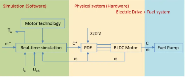
2.2 Actual need of HIL
The physical plant of HIL, which is presented on the Figure 1, contains the electric motor with its power drive electronics (PDE), the fuel pump and the fuel metering unit (the fuel system components are kept to reuse a mature technology). On the other hand, the real electric motor is taken commercially-off-the-shelf and is chosen without any constraints of airworthiness. In the present study, the real electric motor has been chosen among 60 suppliers datasheets to display high performance (low inertia,
torque/power capability suited to the estimated need with sufficient margin).
The main interest of the proposed HIL comes from the possibility to force the real electric motor to operate like a given motor, the virtual motor that is representative of the effective motor that would be specified, designed, manufactured and installed on the engine. The model of the virtual motor is developed in order to be consistent with real-time simulation constraints (e.g. sampling period between 1 and 5 ms). The provided torque is calculated by real-time simulation as a function of its rotor velocity and of the command signal. It is then sent to the real motor drive as a torque setpoint (torque bandwidth greater than e.g. 1000 Hz). The real motor speed is measured to feed the simulation model.
Figure 1: HIL structure
The virtual motor model is developed in order to simulate the following effects:
Power capability (torque vs. velocity) Dynamics (of drive, effect of motor inertia) Energy consumption
Temperature of the windings and motor frame, vs environment conditions, with impact
Response to fault (e.g. short circuit of windings or open leg of inverter)
Impact to the drive architecture and control (brushed/brushless motor, 6-step or field oriented control, sensorless speed control, etc.)
Impact of the engine starting strategy (e-pump, starter, igniter, etc.).
3 Selection of electric motor
One of the most important driver to use HIL methodology here is the uncertainty that affects the selection of appropriate electric motor for the intended application. As mentioned before, there are at least five electric motor technologies that can be used in our application. Figure 2 summarizes most used electric motor in Hybrid and Electric Vehicles and their appropriate PDE:
Figure 2: PDE versus motor type
Indeed, the most important factors in choosing a motor according to [16] are weight, efficiency and cost. These factors can be combined with application requirements. For example, AC motor which the best motor for Hybrid and Electric Vehicles is no more a good choice for aeronautics application because of its mass, which can be twice that of PMSMs or BLDCs motors, without their PDE, [16].
Concerning the present application, the required motor has to supply a continuous nominal torque typically 0.5 N.m and its maximum speed is 10000 rpm. Electric power supply is imposed by aerospace standards. A wide search has been done for different types of electric motors, among 60 off-the-shelf references (25 BLDC, including 5 pancake hollow shaft, 17 DC, 12 AC), there were only 5 as potential candidates even though they did not meet all required criteria. Furthermore, some suppliers of potential motors needed a business plan to accept delivering a few samples, which was not available at this stage of the project.
For these reasons, HIL was selected as a methodology to test different motor designs and help to facilitate the development of the electrically-driven pump.
Ref Real part Virtual (simulated) Part Objective of HIL [8] Electric drive + Motor emulating
the hydraulic pump with PDEs
Hydraulic system (components of hydraulic mobile machine, ex. Industrial forklift)
To simplify the components choosing and testing for new hydraulic system
[14] and [15]
Electric drive + Motor emulating the hydraulic pump with PDEs
Hydraulic and mechanical components of hybrid drive of off-road mobile machinery
To choose the optimum electric motor that emulates the hydraulic pump. According to required refresh rate of electric motor’s torque control loop, motor parameter limit values are suggested for required motor
[13] Electric drive + Motor emulating the hydraulic pump with PDEs
Hydraulic Pump To get more information about system performance at different working conditions
This paper
High performance electric drive + Real hydraulic pump
Virtual drive (supply, motor, and PDE) to be used in the final product
To test different electric motor technologies, observe limitation and give recommendations to get optimum electric drive
4 HIL configuration
As it is described previously, HIL contains two parts; the first one is the software part which contains a real-time model representing a tested virtual electric motor and its drive. Moreover, many submodels can be developed to predict performance at different operation conditions. As addressed later, this can help to test the effect of supply voltage and thermal equilibrium of the simulated motor. The second one is the hardware part. The real motor is used to drive the load under test according to the simulated motor characteristic. A second real motor is used in the present case in order to load the first motor without waiting the real fuel pump and fuel metering to be available for testing. The test bench hardware includes the two motors and their PDE, additional torque/speed/temperature sensors, displays, two computers (PC for configuration and data analysis and PC to run real-time submodels) and real-time target machine which interfaces with PDEs and sensors and runs the real-time simulation.
Figure 3 shows a simple representation of HIL configuration:
Figure 3: Simple representation of HIL configuration
5 Software (Modelling of different submodels)
The real-time model contains essentially a model of simulated electric motor. The complexity of this model can be increased step-by-step (as far as real-time constraints are met) by integrating other sub models, in order to reproduce different aspect that affects motor performance. In this paper, a thermal model is presented to take into account the effect of temperature on the motor performance, including its impact on windings resistance or heat exchange with surrounding environment. Second presented submodel is used to assess the effect of power supply variations. Figure 4 displays how these models interface through power variables: voltage and current delivered by electric supply (Uob, I), heat power and motor temperature (Plosses, Tw).Figure 4: Different submodels developed for real-time simulation
5.1 Modelling of electric motor
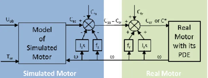
As the main interest of the proposed HIL approach is to force the real electric driving motor on the test bench to operate like any given motor, named the simulated or the virtual motor. Therefore, the shaft torque of the two motors is identical, as far as friction and inertia of the coupling element are negligible with respect to the rated torque. The approach is illustrated for two motor technologies, DC motor and AC motor as virtual motor. The shaft torque of the simulated motor will be transmitted to the driving motor of the test bench as torque setpoint, as presented in Figure 1. Thus, shaft torque of the simulated and real motors shall be identical at any time, as illustrated in Figure 5 and eq. (1):
𝐶𝑠𝑠= 𝐶𝑠𝑟 (1)
with Css, Csr are shaft torque of simulated motor and real motor (N.m), respectively.
On a motor, the shaft torque equals to the electromagnetic torque minus the dissipative torque due to friction and the inertial torque due to the rotor inertia. Assuming the speed to not reverse in the present pump drive application and friction to be made of pure Coulomb and viscous effects brings, as presented in (2):
C𝑠𝑠 = 𝐶𝑒𝑠− 𝑓𝑠𝜔 − 𝐶𝑓𝑠− 𝐽𝑠𝜔̇
C𝑠𝑟= 𝐶𝑒𝑟− 𝑓𝑟𝜔 − 𝐶𝑓𝑟− 𝐽𝑟𝜔̇
(2)
with Ce electromagnetic torque produced by the motor (N.m), f coefficient of viscous friction (N.m.s/rad), Cf Coulomb friction torque (N.m), J inertia of the motor rotor (Kg.m2), rotary speed of the motor shaft (rad/s), 𝜔̇ motor shaft angular acceleration (rad/s2). Subscripts r and s are associated with the real and the simulated motors, respectively.
Thus, according to (1) and (2), the electromagnetic torque setpoint which will be sent to the real motor drive is:
𝐶∗= 𝐶
𝑒𝑟= 𝐶𝑒𝑠− (𝐶𝑓𝑠− 𝐶𝑓𝑟) − (𝑓𝑠− 𝑓𝑟)𝜔 − (𝐽𝑠
− 𝐽𝑟)𝜔̇
(3)
with C* electromagnetic torque setpoint (N.m)
Figure 5 represents a simplified torque calculation for two motors:
Figure 5: Simplified representation of the torque calculation for the simulated and real motors
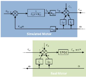
5.1.1 Simulation of a DC Motor
The electromagnetic torque of the simulated permanent magnets DC motor is:
C𝑒𝑠= 𝐾𝑚𝑠𝐼𝑠 (4)
with Kms torque constant of simulated motor (N.m/A), Is current supplied to the simulated motor (A). This current can be calculated from eq. (5):
𝑈𝑜𝑏 = 𝐾𝑚𝑠𝜔 + 𝑅𝑠𝐼𝑠+ 𝐿𝑠
𝑑𝐼𝑠
𝑑𝑡 (5)
with Uob voltage supplied to simulated motor (V), Rs and Ls rotor windings electrical resistance () and inductance (H) of simulated motor, respectively.
From equations (3) (4) and (5), the electromagnetic torque setpoint becomes: 𝐶∗= 1 𝐻(𝑠)[𝐾𝑚𝑠 1 𝑅𝑚𝑠+ 𝐿𝑚𝑠𝑠(𝑈𝑜𝑏− 𝐾𝑚𝑠𝜔) − −(𝐶𝑓𝑠− 𝐶𝑓𝑟) − (𝑓𝑠− 𝑓𝑟)𝜔 − (𝐽𝑠− 𝐽𝑟)𝜔̇] (6)
with H(s) dynamics of the real motor PDE torque loop. Eq. (6) can be presented in block diagram as in Figure 6:
Figure 6: Calculation of the electromagnetic torque setpoint for the simulation of a DC motor
5.1.2 Simulation of an AC Motor (Induction type)
The next virtual motor to be tested as virtual motor is a three phase induction motor.
First of all, a static model is used to reproduce the motor torque-speed characteristics. Then, a dynamic model is tested to induce an electromagnetic torque as a function of motor current and parameters.
In the first model, the motor torque is extracted from characteristics curve presented in motor datasheet as a
function of motor speed. These data can be implanted as a data table in the real-time model.
Concerning the second model, the motor torque is calculated as a function of current in Park’s coordinates. According to [17] [18] the electromagnetic torque in squirrel cage AC motor is given by:
𝐶𝑒𝑠=
3 2 𝑃
2𝐿𝑚(𝑖𝑞𝑠𝑖𝑑𝑟− 𝑖𝑑𝑠𝑖𝑞𝑟) (7)
with P number of poles, Lm mutual or magnetizing inductance (H), i motor current (subscript s is for stator current, r for rotor, d for direct axis and q for quadrature axis in Park’s coordinates).
These currents can be calculated as a function of motor design parameters, such as rotor inductance, stator inductance, mutual inductance, flux linkage in the motor and electrical speed of the rotor, as it is presented in [17] [18].
5.2 Thermal model
5.2.1 Importance of thermal analysis
Thermal performance analysis of electric motors is a crucial step during design phase to insure long lifetime and reliable performance of the motor. Indeed, electric machines lifetime is specified by temperature at which their winding electrical insulations are exposed, which is for example (85°C, 100°C, 125°C, 155°C) [19]. So, higher temperature means shorter motor lifetime, and vice versa, where motor lifetime is reduced to half each time the temperature increases 10°C above its value at which the lifetime is calculated. For instance, if a motor has a normal lifespan of 8 years at an average temperature of 105 °C, it becomes 4 years at 115 °C, 2 years at 125 °C and one year only at 135 °C [20]. Not only motor lifetime is affected by temperature, but also its performance fluctuates with motor electromagnetic parameters variation versus temperature. For instance, the permanent magnets induction decreases by 4% for SmCo5
and by 12% for sintered NdFeB when their temperature increases about 100°C. Similarly, the resistance of copper winding increases by 42% when its temperature increases by 100°C. The convective heat exchange coefficient for horizontal exchange surface at 20°C ambient increases by 38% as the exchange surface temperature rises from 50°C to 150°C, and finally the voltage drop at rated current and commutation energy for one IGBT, a widely used power transistor in PDE, rises by 25% as its temperature changes from 25°C to 125°C [21] [22].
In fact, thermal analysis is a quite complex phenomena because electromagnetic losses increase motor temperature, so motor parameters such as electric resistance R and induction B (density of flux magnetic) will change with temperature, as eq. (11) illustrates. As a result, copper losses will increase with the increasing of electric resistance and also iron losses with induction rise, which leads to more heating, and the loop continues, making a snowball effect.
At last and not least, thermal analysis is helpful to detect fault in the motor, which occurs if the temperature exceed its estimated value in normal operation, as in [23].
5.2.2 Electric motor losses
Losses are the main sources of heating in the electric machines. Generally in electric motors, the main losses are cooper losses, also known as Joule power losses, which depends on coil current and ohmic resistance, it can reach 30% of input power [19]. In second place are iron losses, which contain eddy current losses and hysteresis losses and depend on motor rotational speed. They can reach about 10-20% of the rated torque [19]. In third place, mechanical losses present as friction losses in bearings and at graphite brushes for DC motors, which is proportional to motor rotational speed, and viscous friction of rotor in the air-gap which is proportional to square of motor speed [24]. Brushes friction losses of graphite brushes are about 5% of rated torque but they are less that value for precious metal brushes [19].
Furthermore, stray losses which regroup electromagnetic losses that cannot be classified in previous losses. They occur for different raisons, for example because of a non-uniform current distribution in copper winding or because of the magnetic flux which is produced by the load current and which leads to additional iron losses. Generally, it is considered as a percentage of output power (3 to 5%) for small electric machine (less than 10kW) [25].
Brush losses disappear in permanent magnet BLDC motor where the dominant losses are electromagnetic losses, which combine copper and iron losses. For example, it is about 80% of total losses whereas bearing losses are about 12%, going up with increasing motor speed or load [26]. However, friction losses are neglected in most of studies of permanent magnet synchronous machines (PMSM), like in [27][28].
In this paper, motor total losses are divided into two parts, the first on is copper losses and the second one is stator iron losses which integrated frictional losses. Heat generated in permanent magnets from viscous friction losses are supposed small in comparison with iron losses. Next equations present PMSM losses [29] :
𝑃𝐶𝑢= 3 𝑅∅𝐼∅ 𝑟𝑚𝑠2 𝑃𝐹𝑒= 𝑃ℎ𝑦𝑠+ 𝑃𝑒𝑑 𝑃ℎ𝑦𝑠= 𝑘ℎ𝑦𝑠𝐵𝑚𝑎𝑥2 𝑓 𝑃𝑒𝑑 = 𝑘𝑒𝑑𝐵𝑚𝑎𝑥2 𝑓2 𝑃𝑙𝑜𝑠𝑠𝑒𝑠= 𝑃𝐶𝑢+ 𝑃𝐹𝑒 (8)
with Plosses total losses in electric motor (W), PCu copper losses (W), PFe iron losses (W), Phys magnetic hysteresis losses (W), Ped eddy current losses (W), R electrical resistance of one phase (), I current of one phase (A), Bmax
maximum flux density (T), f frequency flux variation (Hz),
khys hysteresis constant and ked eddy current constant.
khys, ked are constants determined by the manufacturer provided loss data (khys is a constant whose value depends on the ferromagnetic material and the volume of the core. ked is a constant whose value depends on the type of material and its lamination thickness [30]).
5.2.3 Thermal model with constant electrical resistance
The objective here is to show the ability to integrate the thermal model in the HIL real-time model. Considering the selected environment, the thermal model will be presented in form of block diagram which facilitates its integration with the global real-time model in Matlab/Simulink.
A simple thermal model is given by: 𝑃𝑙𝑜𝑠𝑠𝑒𝑠= 𝑃𝑅+ 𝑃𝐶 𝑃𝑙𝑜𝑠𝑠𝑒𝑠= ∆𝑇 𝑅𝑡ℎ+ 𝐶𝑡ℎ 𝑑 𝑑𝑡(∆𝑇) (9)
with PR exchanged heat power with surrounding environment and PC (W) stored heat power in thermal capacitance, Rth thermal resistance (°K/W), Cth thermal capacity (J/°K) and T temperature difference between domain and environment (°K).
The heat power exchange is split in 2 parts; with the ambient
Pa and with the hydraulic pump Pp. It is assumed at first that the first exchange occurs by natural convection and the second one is by conduction.
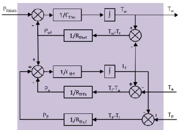
The simplest thermal model is to consider the whole motor as a single body. Nevertheless, the presented thermal model studies the winding separately from the motor frame. So, it has two thermal capacitances, Cthw for winding and Cthf for frame. The propagation of heat flow in the motor is from hot winding, towards the frame by conduction then to ambient through natural convection. So, the two bodies thermal model is presented in (10) and Figure 7:
𝑃𝑙𝑜𝑠𝑠𝑒𝑠− 𝑃𝑤𝑓 = 𝐶𝑡ℎ𝑤 𝑑𝑇𝑤 𝑑𝑡 𝑃𝑤𝑓+ 𝑃𝑝− 𝑃𝑎= 𝐶𝑡ℎ𝑓 𝑑𝑇𝑓 𝑑𝑡 𝑃𝑤𝑓 = 1 𝑅𝑡ℎ𝑤𝑓(𝑇𝑤− 𝑇𝑓) 𝑃𝑓𝑎= 1 𝑅𝑡ℎ𝑓𝑎(𝑇𝑓− 𝑇𝑎) 𝑃𝑝𝑓= 1 𝑅𝑡ℎ𝑝𝑓(𝑇𝑝− 𝑇𝑓) (10)
with Rthwf, Rthfa, Rthpf thermal resistances between windings and motor frame, between motor frame and ambient, between the pump and the motor frame (°K/W),
respectively. Cthw, Cthf are thermal capacitance of motor winding and motor frame (J/°K), respectively. Tf, Tw, Ta, Tp are temperatures of motor frame, motor winding, ambient and pump (°K), respectively.
Two bodies thermal model of an electric motor is presented in Figure 7:
Figure 7: Block diagram of two bodies thermal model of an electric motor
The PDE losses are beyond the objective of the reported work.
5.2.4 Thermal model with varied electrical resistance
The electrical resistance and all electric motor parameters mentioned in the datasheet are measured at a constant temperature, named catalog temperature TC which usually
equals 25°C. Nevertheless, as mentioned before, electric resistance, as many other motor parameters, varies with motor operating temperature. It can be calculated as a function of its reference value R(TC), at reference TC and
winding temperature TW as in eq. (11).
𝑅(𝑇𝑤)= 𝑅(𝑇𝑐)[1 + 𝛼𝑐𝑜𝑝𝑝𝑒𝑟 (𝑇𝑤− 𝑇𝐶)] (11)
with R(Tw) and R(TC) electrical resistance at actual temperature Tw and catalog temperature TC in (), respectively. copper is
temperature coefficient of winding, which is equal to 0.0039 (°K-1) for copper.
Figure 8 represents thermal model of electric motor with temperature sensitive windings resistance:
Figure 8: Block diagram of thermal model with temperature sensitive windings resistance
There is no special issue to consider the influence of temperature on magnetic induction. The process to modify the original model is Figure 7 remaining unchanged.
5.3 Model of power supply of on-board network
Another objective of the present work was to assess the impact of supply power. In the considered application, the on-board power supply is continuous DC voltage delivered by battery, according to the MIL_STD_704F and RTCA-DO160F standards [31], [32].
The supplied voltage is not constant, in particular if other consumers (e.g. starter) draw high power during the operation of the motor under study. This dynamic change of supply voltage is particularly important, especially if the electric motor is to be simulated is supplied directly without PDE.
The following intends to illustrate with a simple example how the supply conditions can be introduced in the simulated drive. Generally, the power supply of electrical on-board network depends on battery voltage, its internal resistance and the consumed current, as mentioned in (12):
𝑈𝑜𝑏= 𝑈𝑏𝑎𝑡− 𝑅𝑖 𝐼 (12)
with Uob power supply of the on-board electrical network (VDC), Ri internal resistance of the battery () and I consumed current in the electrical circuit (A). This current represents the sum of electrical currents consumed by different electrical devices supplied.
This can be implemented extending the model of Figure 7 as given in Figure 9:
Figure 9: Simple model of on-board power supply
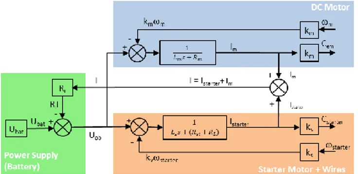
A major power consumer is the engine DC starter that is simple starter DC motor, which turns-on when the studied electric pump motor is running. The consumed current is:
𝐼 =𝑈𝑏𝑎𝑡− 𝑘𝑠𝜔𝑠𝑡𝑎𝑟𝑡𝑒𝑟
𝑅𝑖+ 𝑅𝐿+ 𝑅𝑠 (13)
with RL, Rs electrical resistance of network cables and of starter motor (), respectively, starter and ks the rotary speed (rad/s) and motor constant (V.s/rad) of the starter motor. Thus, the block diagram model of the effective supply conditions of the motor under study can be added as illustrated by Figure 10:
Figure 10: Model of power supply including battery, wires and starter motor (as an example)
5.4 Hardware configuration
A specific test bench has been designed to support the assessment of the proposed HIL approach. Its architecture has been introduced in Figure 11 and Figure 12. It consists of :
A mechanical assembly with the frame that supports the driving and loading motors. The two motors are connected face to face by means of mechanical couplings and torque transducer, Figure 12.
The rack with two motors PDEs and the electric supply unit (ESU).
The real-time simulator, which consists of a personal computer for configuration and data analysis and a real-time board which interfaces with the PDE and the sensor and runs the real-time model.
Figure 11: Test bench hardware
Used motors are off-the-shelf commercial BLDC motors from ABB. Rated torques are 0.9 N.m and 1.36 N.m for the driving and loading motors, respectively. The motors were chosen for their low rotor inertia (0.124 Kg.cm2 and 0.18 Kg.cm2) in order to facilitate the emulation of other motors (see equation 6).
Figure 12: Two electric motors assembly
The two PDE are identical, “Microflex e150” with rated of current of 6A. Interfaces with the real-time board are either analogue or through EtherCAT bus.
The torque transducer was selected from “Magtrol” with rated torque of 5 N.m and maximum speed of 20000 rpm. Suitable couplings were picked from the same supplier “Magtrol” to protect against the effects of misalignment. The real-time target machine is “Speedgoat” which has IntelCore2Duo 2.26 GHz processor, 2048 MB RAM and with an analog input and output I/O module 102 and EtherCAT interface. The real-time models were developed and uploaded on the target machine within the Matlab-Simulink simulation environment.
6 Test results and lessons learned
6.1 Experiments
The first simulated drive was brushed DC motor that was directly connected to the simulated DC supply without any PDE. The motor was Maxon 353295 (rated output power 250 W, nominal voltage 24V, nominal speed is 3810 rpm, nominal torque 0.501 N.m and inertia 1.29 Kg.cm2). The simulated drive was implemented as presented on Figure 6. An AC motor was also simulated as a Woodward AC motor (4 poles, frequency 400 Hz, synchronous speed 12000 rpm, and inertia 9.8 Kg.cm2).
For all real-time simulations, the sampling rate was 1 ms. The average TET (total elapsed time) to run the models did not exceed 0.0213 ms with a max value lower than 0.026 ms.
6.2 Lessons learned
The reported work intended to use of-the-shelf hardware to implement a HIL platform for emulating a motor drive. The experience acquired can be summarized in terms of lessons learned and recommendations that concerns mainly the hardware: a) Static accuracy RT target machine ESU+PDEs 2 EM assembly RT simulation PC Configuration PC Displays RT target machine display
Electric motors Couplings
Torque transducer
The torque produced by the real motor at shaft interface is far different from the electromagnetic torque produced by its PDE. This is due to motor shaft friction (bearings, seals and windage) and motor rotor inertia. PDEs generally include an estimate of these values as a feedforward action in the motor control. Moreover, the current (or torque loop) ignores the effective electromagnetic torque produced as it only uses windings current measurements. Finally, although these effects are compensated in the PDE control algorithm, the motor torque at shaft interface is not accurately related to the torque setpoint, generating errors in the HIL process. This requires an accurate identification of these effects to feed the compensators that can be either implemented in the PDE or in the real-time simulation, as given by equation (6). b) Dynamics
The potential dynamic effects that might be intended to simulate for the virtual drive can be listed from the slowest to the fastest (typically):
Thermal time constant (motor housing to ambient) Motor time constant (windings to housing) Cogging torque effects
Dynamics of position control (not applicable here) Dynamics of speed control
Electric time constant of the motor Dynamics of torque control Sampling
PWM switching
In practice, what can be simulated is constrained by hardware. The real-time platform, a basic one, could run quite complex models at a sampling rate of 0.05 ms. This is consistent with the simulation of motors electric time constant and even torque (or current) loop dynamics. The main limitation came for the industrial electric drive that was used in torque control mode from external setpoint. Whatever the type of data interfacing (analog, digital bus), electric power drives sample the data exchanged (here torque setpoint input and effective velocity output) at 1 ms to 5 ms. This is the main limitation factor for simulating highest dynamics. The best option is definitely to input the torque demand directly at the PWM input to take benefit of its high frequency, typically 8 kHz to 16 kHz (62.5 s to 125 s).
c) Difference in motor rotor's inertia
As pointed out by equation (6), the torque setpoint involves the compensation of the difference between the simulated motor and the effective motor rotors inertia. Consequently, the measured rotor speed signal has to be time-derivated to calculate this member. Unfortunately, the speed signal is generally noisy and cannot be differentiated without noise (or phase lag if filtered efficiently). As for loading test benches, the best approach when possible is to use a real motor with the lowest inertia and to increase it through
additional bodies to exactly reproduce the inertia of the simulated motor. In practice, this option is not always easy to implement as the used motor has to be interfaced with the real load, generally through adaptation joints that increase inertia (especially if a torque transducer is inserted). This is a severe limitation.
d) Causality
The proposed implement of HIL consists in generating the torque setpoint demand as a function of actual measured rotor velocity. This solution was logically selected as the torque loop is faster than the speed loop. However, the other option was tested that consisted in generating the speed demand as a function of the transmitted torque. As anticipated, performance was extremely low, due to the impact of the real motor speed loop dynamics.
7 Conclusion
The present paper has dealt with hardware in the loop (HIL) as a methodology to support the specification of electric drives in the presence of high uncertainty on the driven load power characteristic. It was intended to drive the load with off-the-shelf high performance BLDC motor and power drive electronics to emulate the candidate electric drive. The approach was applied to an electrically-driven fuel pump. The first part of the paper introduced the proposed HIL architecture that consists in simulating in real-time the emulated electric drive and supply by generating the motor torque to be developed on the driven load as a function of the motor shaft angular velocity. Simple examples have been provided to illustrate how the supply conditions, the motor dynamics and the thermal effects can be included in the real-time simulation.
It was shown that there is no issue in reproducing the motor steady-state power characteristic as well as the thermal effects that significantly impact the electric drive sizing and effective service life. However, three main lessons have been learned and come from the limitations introduced by hardware. First, the used motor has to be identified with care. This is mandatory to get the expected torque at shaft through accurate compensation of friction, inertia and current/torque characteristic. Secondly, industrial power drive electronics sampling of setpoint and measured signals (1 to 5 ms typically) strongly limit the ability to simulate in real-time the motor dynamics. Oppositely, real-time hardware was not found to be limitative as models could be simulated with only a few tenths of microseconds step. Last, the difference between the inertia of the simulated and the used motor rotors is difficult to compensate efficiently due to noise or phase lag effect. It is therefore recommended to setup the test bench in such a way that the effective rotor inertia equals the simulated motor one.
Acknowledgement
The present work has been funded by Region Occitanie and Fonds Unique Interministériel in the frame of the 18th project call n°15061455.
Nomenclature
Designation Denotation Unit
C* Torque setpoint N.m
copper
Temperature coefficient of
copper winding K°
-1
Shaft rotary speed rad/s
starter Rotary speed of the stator motor rad/s
𝜔̇ Derivative of shaft rotary speed rad/s2 T Temperature difference between studied points K°
Bmax Maximum flux density T
Cer
Electromagnetic torque
produced by real motor N.m
Ces
Electromagnetic torque
produced by simulated motor N.m
Cfr Dry friction torque in real motor N.m
Cfs
Dry friction torque in simulated
motor N.m
Csr Shaft torque of real motor N.m
Css Shaft torque of simulated motor N.m
Cth Thermal capacity J/K°
Cthf
Thermal capacity of motor
frame J/K°
Cthw
Thermal capacity of motor
winding J/K°
f Frequency flux variation rad/s
fr
Coefficient of viscous friction in
real motor N.m.s/rad
fs
Coefficient of viscous friction in
simulated motor N.m.s/rad
I Consumed current in the
electrical circuit A
I Current of one phase A
idr d-axis rotor current A
ids d-axis stator current A
iqr q-axis rotor current A
iqs q-axis stator current A
Is current in simulated motor A
Jr Inertia of real motor Kg.m2
Js Inertia of simulated motor Kg.m2
ked Eddy current constant
khys Hysteresis constant
Kms Constant of simulated motor N.m/A
ks
Motor constant of the stator
motor V.s/rad
Lm
Mutual or magnetizing
inductance in AC motor H
Ls Inductance of simulated motor H
P Number of AC motor poles pole
Pa Heat exchange with the ambient W
PC Stored heat in thermal capacitor W
PCu Copper losses W
Ped Eddy current losses W
PFe Iron losses W
Phys Hysteresis losses W
Plosses Total losses in electric motor W
Pp
Heat exchange with the
hydraulic pump W
PR
Exchanged heat with
surrounding environment W
R Electrical resistance of one phase
R(T)
Electrical resistance at actual
temperature T
R(TC)
Electrical resistance at catalog
temperature TC
Ri Internal resistance of the battery
RL
Electrical resistance of network
cables
Rs
Electrical resistance of
simulated motor
Rs
Electrical resistance of starter
motor
Rth Thermal resistance °K/W
Rthfa
Thermal resistance between
motor frame and the ambient °K/W
Rthpf
Thermal resistance between the
pump and the motor frame °K/W
Rthwf
Thermal resistance between the
winding and the frame °K/W
Ta Temperature of ambient °K
Tc
Temperature considered in
catalog parameters °K
Tf Temperature of motor frame °K
Tp Temperature of pump °K
Uob
Power supply of the on-board
electrical VDC
References
[1] J. German, “Hybrid vehicles: Trends in technology development and cost reduction,” International
Council on Clean Transportation, Technical Brief,
no. 1, pp. 1–18, 2015.
[2] M. H. Rashid, Power Electronics Handbook,
Devices, Circuits and Applications, 3 rd. USA:
ELSEVIER, 2011.
[3] F. Jian, “Incremental Virtual Prototyping of Electromechanical Actuators for Position Synchronization,” INSA de Toulouse, 2016.
[4] M. Zeraoulia, M. E. H. Benbouzid, and D. Diallo, “Electric Motor Drive Selection Issues for HEV Propulsion Systems: A Comparative Study,” IEEE
Transactions on vehicular technology, vol. 55, no. 6,
pp. 1756–1764, 2006.
[5] F. Badin, Les Véhicules Hybrides des composants
au système. Editions TECHNIP, 2013.
[6] C. Köhler, “Enhancing Embedded Systems Simulation, A Chip-Hardware-in-the-Loop Simulation Framework,” VIEWEG+ TEUBNER RESEARCH, 2010.
[7] L. I. N. Cheng and Z. Lipeng, “Hardware-in-the-loop Simulation and Its Application in Electric Vehicle Development,” in IEEE Vehicle Power and
Propulsion Conference (VPPC), September 3-5,
2008.
[8] J. E. Heikkinen, T. A. Minav, J. J. Pyrhonen, and H. M. Handroos, “Real-time HIL-simulation for testing of electric motor drives emulating hydraulic systems,” International Review of Electrical
Engineering, vol. 7, no. 6, pp. 6084–6092, 2012.
[9] H. K. Fathy, Z. S. Filipi, J. Hagena, and J. L. Stein, “Review of Hardware-in-the-Loop Simulation and Its Prospects in the Automotive Area,” Modeling
and Simulation for Military Applications, vol. 6228,
no. E, 2006.
[10] O. A. Mohammed and N. Y. Abed, “Real-time simulation of electric machine drives with hardware-in-the-loop,” COMPEL: The International Journal
for Computation and Mathematics in Electrical and Electronic Engineering, vol. 27, no. 4, pp. 929– 938,
2008.
[11] J. J. Poon, M. A. Kinsy, N. A. Pallo, S. Devadas, and I. L. Celanovic, “Hardware-in-the-Loop Testing for Electric Vehicle Drive Applications,” Applied
Power Electronics Conference and Exposition (APEC), Twenty-Seventh Annual IEEE, pp. 2576–
2582, 2012.
[12] C. Choi, K. Lee, and W. Lee, “Design and Temporal Analysis of Hardware-in-the-loop Simulation for Testing Motor Control Unit,” Journal of Electrical
Engineering & Technology, vol. 7, no. 3, pp. 366–
375, 2012.
[13] V. Vodovozov, L. Gevorkov, and Z. Raud, “Modeling and Analysis of Pumping Motor Drives
in Hardware-in-the-Loop Environment,” Journal of
Power and energy Engineering, vol. 2, pp. 19–27,
2014.
[14] J. E. Heikkinen, T. Minav, H. M. Handroos, J. A. Tapia, and J. Werner, “Modelling study of an optimum electric motor for directly driven hydraulic pump emulator in real- time HIL-simulation,” in The
Fourteen Scandinavian International Conference on Fluid Power, May 20-22, 2015.
[15] J. E. Heikkinen, T. A. Minav, H. M. Handroos, and J. A. Tapia, “Electric motor based hydraulic motor pump emulator in real time HIL-simulation : Finding the optimum emulator electric motor,” in
Proceeding of the 8th FPNI Ph.D Dymposium on Fluid Power, FPNI, June 11-13, 2014.
[16] J. G. W. West, “DC, induction, reluctance and PM motors for electric vehicles Electric,” Power
Engineering Journal, vol. 8, no. 2, pp. 77–88, 1994.
[17] A. W. Leedy, “Simulink / MATLAB Dynamic Induction Motor Model for Use as A Teaching and Research Tool,” International Journal of Soft
Computing and Engineering (IJSCE), vol. 3, no. 4,
pp. 102–107, 2013.
[18] A. W. Leedy, “Simulink / MATLAB Dynamic Induction Motor Model for use in Undergraduate Electric Machines and Power Electronics Courses,” in 2013 Proceedings of IEEE Southeastcon, 4-7
April, 2013.
[19] Maxon Motor, “Thermal Calculations of Motors.” Maxon Academy, Swizerland, 2009.
[20] W. Théodore, Electrotechnique, 3e édition. Canada: De Boeck Université, 2000.
[21] M. Jean-Charles, Aerospace Actuators, Vol 2,
Signal-by-Wire/ Power-by-Wire. Wiley, 2016.
[22] S. Constantinides, “Understanding and Using Reversible Temperature Coefficients,” in
MAGNETICS 2010, January 28-29, 2010.
[23] L. I. Silva, P. M. De La Barrera, C. H. De Angelo, F. Aguilera, and G. O. Garcia, “Multi-Domain Model for Electric Traction Drives Using Bond Graphs,” Journal of Power Electronics, vol. 11, no. 4, pp. 439–448, 2011.
[24] G. LACROUX, Les actionneurs électriques pour la
robotique et les asservissements, 2e édition.
Technique et Documentation LAVOISIER, 1994. [25] P. Andrada, M. Torrent, J. I. Perat, and B. Blanqué,
“Power Losses in Outside-Spin Brushless D . C . Motors,” Renewable Energy & Power Quality
Journal (RE & PQJ), vol. 1, no. 2, pp. 507– 511,
2004.
[26] J. Kuria and P. Hwang, “Modeling Power Losses in Electric Vehicle BLDC Motor,” Journal Of Energy
Technologies and Policy, vol. 1, no. 4, pp. 8–17,
2011.
[27] M. A. FAKHFAKH, M. HADJ KASEM, S. TOUNSI, and R. NEJI, “Thermal Analysis of Permanent Magnet Synchronous Motor for Electric Vehicles,” Journal of Asian Electric Vehicles, vol. 6, no. 2, pp. 1145–1151, 2008.
ANALYSIS OF A PMSM USING FEA AND LUMPED PARAMETER MODELING ANALIZA CIEPLNA SILNIKA PMSM ZA POMOCĄ METODY ELEMENTÓW SKOŃCZONYCH,”
Technical Transactions, Electrical Engineering, vol.
1, no. E, pp. 97–107, 2015.
[29] E. Andersson, “Real time thermal model for servomotor applications,” 2006.
[30] P. C. SEN, PRINCIPLES OF ELECTRIC MACHINES AND POWER ELECTRONICS, Third
edit. USA: WILEY, 2014.
[31] “RTCA DO-160F, Environmental Conditions and Test Procedures for Airborne Equipement, Section 16, Power input,” 2007.
[32] “Military Standard, Aircraft Electric Power Characteristics, MIL-STD-704F,” 2013.
![[PDF] Premières leçons de programmation en turbo Pascal | Cours informatique](data:image/gif;base64,R0lGODlhAQABAIAAAP///wAAACH5BAEAAAAALAAAAAABAAEAAAICRAEAOw==)