Optimal Gabor Filter Parameters Selection using Genetic Algorithms

(1)

؀ ؀؀

؀

؀ ؀

؀

Democratic and Popular Republic of Algeria

Ministry of Higher Education and Scientific Research

Ahmed Draia University - Adrar

Faculty of Science and Technology

Department of Mathematics and Computer Science

A Thesis Presented to fulfill the Master Degree in Computer Science

Option: Intelligent Systems

Title:

Optimal Gabor Filter Parameters Selection using Genetic

Algorithms: Application of Content based Image Retrieval

Prepared by

Marwa MORSLI and Hadjer MOULAY OMAR

Jury Members:

Dr. Elmamoun Mamouni

President

Mr. Mohammed Kohili

Examiner

Pr. Mohammed Omari

Supervisor

(2)

Abstract

Content based image retrieval (CBIR) systems use the contents of image such as color, texture and shape to represent and retrieve images from large databases. In this thesis, we present a CBIR system based on integration of both color and texture feature. Due to the poor distinguishing power of color histogram, we have used color moments and color correlogram, which encode some spatial information. They are used to extract the color feature from the image. Gabor filter is used in image retrieval to represent the texture feature. In our work, we try to enhance Gabor filter efficiency using a meta-heuristic optimization: Genetic Algorithms. The similarity of combined features is calculated using Manhattan distance measure. A comparison study of the proposed method with other conventional methods is also presented in this manuscript and experimental results show that the proposed method has good results.

Key terms—CBIR; color moments; color correlogram; Gabor filter; Manhattan distance.

Résumé

Les systèmes d'extraction d'images basés sur le contenu (CBIR) utilisent le contenu de l'image comme la couleur, la texture et la forme pour représenter et récupérer des images à partir de grandes bases de données. Dans ce mémoire, nous présentons un système CBIR basé sur l'intégration de la couleur et de la texture. En raison du faible pouvoir de distinction de l'histogramme de couleur, nous avons utilisé des moments de couleur et un corrélogramme de couleur, qui codent certaines informations spatiales. Ils sont utilisés pour extraire la caractéristique de couleur de l'image. Le filtre Gabor est utilisé dans la récupération d'image pour représenter la propriété de texture. Dans notre travail, nous essayons d'améliorer l'efficacité des filtres de Gabor en utilisant une optimisation méta-heuristique: les algorithmes génétiques. La similarité des caractéristiques combinées est calculée à l'aide de la mesure de distance Manhattan. Une étude comparative de la méthode proposée avec d'autres méthodes conventionnelles est également présentée dans ce manuscrit et les résultats expérimentaux montrent que la méthode proposée donne de bons résultats.

Mots clés —CBIR; Moments de couleur; Correlogramme de couleur; Filtre Gabor; Distance

(3)

ii

Acknowledgements

Firstly, we would like to express my sincere gratitude to our supervisor Pr. Mohammed Omari for the continuous support of our research efforts, for his patience, motivation, and immense knowledge. His guidance helped us throughout all stages of research and writing. We could not have imagined having a better advisor and mentor than him.

Secondly, we thank Mr. Kohili and Dr. Mamouni, the jury members, for accepting to examine this work. We would like also to thank all our teachers at the department of mathematics and computer sciences and our classmates for the amazing journey throughout the last two years. We are really grateful for knowing and learning from you.

Last but not least, we would like to thank our families, our parents, our siblings, and our close friends for supporting us spiritually throughout writing this research work and in life in general.

(4)

Dedicates

We dedicate this modest work:

To our dear parents for their support throughout my life of

study and without which we would never have become what

we are.

To our friends and families.

To all the teachers We have had throughout our schooling

and who have allowed us to succeed in our studies.

To anyone who has contributed to this work from near or

far.

(5)

iv

Table of Content

Abstract ... i Résumé ... i Acknowledgements ... ii Dedicates ... iii Table of Content ... iv

List of Figures ... vii

List of Tables ... ix

List of Abbreviations ... x

Introduction ... 1

Chapter One:Digital Images 1.1 Digital Images ... 4

1.2 Pixels and Bitmaps ... 4

1.3 Types of Digital Images ... 4

1.3.1 Black and White Images ... 5

1.3.2 Color Images ... 6

1.3.3 Binary or Bilevel Images ... 6

1.3.4 Indexed Color Images ... 7

1.4 Common Image File Formats ... 8

1.4.1 TIFF (.tif, .tiff) ... 8

1.4.2 Bitmap (.bmp) ... 8 1.4.3 JPEG (.jpg, .jpeg) ... 8 1.4.4 GIF (.gif) ... 8 1.4.5 PNG (.png) ... 8 1.5 Color Spaces ... 9 1.5.1 RGB ... 9

1.5.2 HSV (Hue Saturation Value) ... 10

(6)

Chapter Two:Image Retrieval

2.1 Process of CBIR ... 14

2.1.1 Feature Extraction ... 15

2.1.1.1 Color Space Selection: ... 15

2.1.1.1.1 Color Feature extraction Method ... 16

2.1.1.2 Texture Feature Extraction... 18

2.1.1.3 Shape Feature Extraction ... 24

2.2 Similarity Measurements: ... 25

2.2.1 The Euclidean distance ... 26

2.2.2 The chamfer distance ... 27

2.2.3 The Manhattan distance ... 27

2.2.4 The Earth Mover Distance ... 27

2.3 Evaluation of unranked retrieval system ... 28

2.3.1 Recall ... 28 2.3.2 Precision ... 28 2.3.3 Inverse Recall ... 28 2.3.4 Inverse Precision ... 28 2.3.5 F-Measure ... 29 2.3.6 Prevalence ... 29 2.4 Related work 1 ... 29

2.4.1 Color Feature Extraction (Phase-I) ... 30

2.4.2 Texture Feature Extraction (Phase II) ... 30

2.4.3 Shape Feature Extraction (Phase II) ... 31

2.5 Related work 2 ... 31

2.6 Proposed Method ... 33

2.6.1 Genetic Algorithm ... 33

2.6.2 Fitness function ... 36

2.6.3 Proposed method ... 37

Chapter Three:Experiments and Results

3.1 Used software and hardware ... Fehler! Textmarke nicht definiert.Erreur ! Signet non

défini.

(7)

vi

3.3 The genetic algorithm functionality .. Fehler! Textmarke nicht definiert.Erreur ! Signet

non défini.

3.3.1 Fitness formula ... Fehler! Textmarke nicht definiert.Erreur ! Signet non défini.

3.4 Results ... Fehler! Textmarke nicht definiert.Erreur ! Signet non défini.

3.4.1 Experiment 1 ... Fehler! Textmarke nicht definiert.Erreur ! Signet non défini. 3.4.2 Experiment 2 ... Fehler! Textmarke nicht definiert.Erreur ! Signet non défini. 3.4.3 Experiment 3 ... Fehler! Textmarke nicht definiert.Erreur ! Signet non défini. 3.4.4 Experiment 4 ... Fehler! Textmarke nicht definiert.Erreur ! Signet non défini. 3.4.5 Experiment 5. ... Fehler! Textmarke nicht definiert.Erreur ! Signet non défini.

3.5 Recall and precision ... Fehler! Textmarke nicht definiert.Erreur ! Signet non défini. 3.6 Discussion ... Fehler! Textmarke nicht definiert.Erreur ! Signet non défini. Conclusion ... 53 References ... 55

(8)

List of Figures

Figure 1: Gray levels 5

Figure 2: Gray scale image example 5

Figure 3: RGB image exemple 6

Figure 4: Binary image example 7

Figure 5: Indexed image example 7

Figure 6: Images formats example 9

Figure 7: The RGB cube viewed from two different directions 10

Figure 8: The HSV color space 10

Figure 9: The HSL color space 11

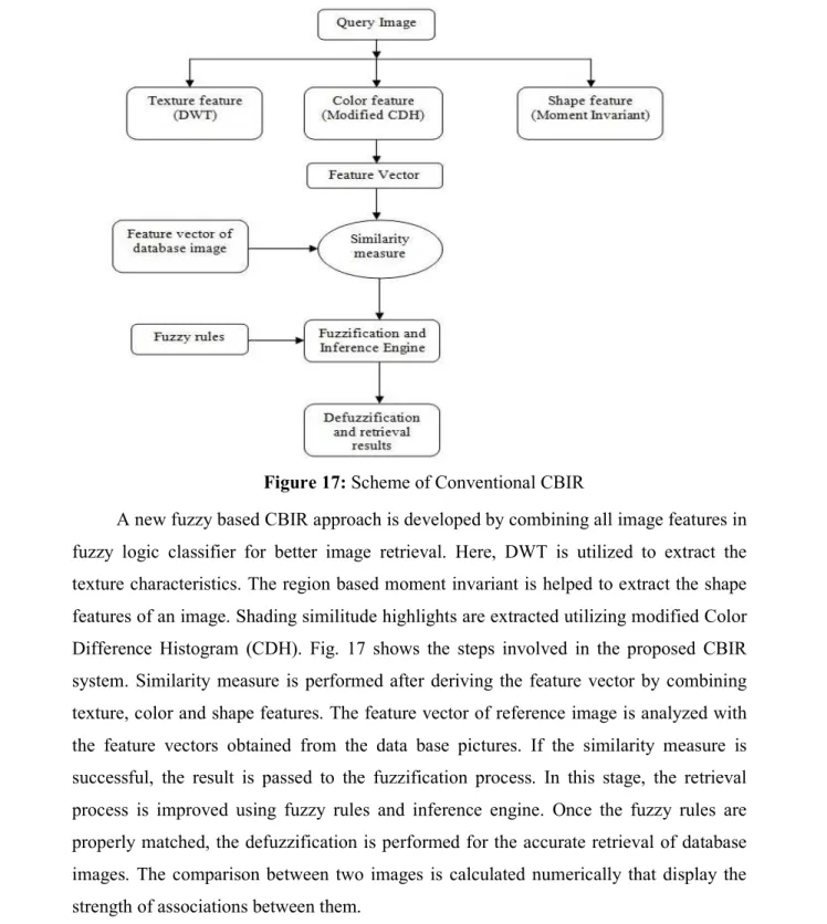
Figure 10: Block diagram of content based image retrieval [6] 14

Figure 11: 2-D Gabor filter obtained by modulating the sine wave with a Gaussian 20

Figure 12 : Keeping other parameters unchanged (Ѐ = 00, Ȁ = 0.25, σ = 10, Ψ = 0), and on

changing the lambda from 30 to 60 and 100 the Gabor function gets thicker 22

Figure 13 : Keeping other parameters unchanged (λ = 30, Ȁ = 0.25, σ = 10, Ψ = 0), and on

changing the theta from 00 to 450 and 900 the Gabor function rotates. 22

Figure 14: Keeping other parameters unchanged (λ = 30, Ѐ = 00, σ = 10, Ψ = 0), and on

changing the gamma from 0.25 to 0.5 and 0.75, the Gabor function gets shorter. 23

Figure 15: Keeping other parameters unchanged (λ = 30, Ѐ = 00 Ȁ = 0.25, Ψ = 0), and on

changing the sigma from 10 to 30 and 45 the number of stripes in Gabor function increases. 23

Figure 16: Block diagram of his proposed retrieval system 29

Figure 17: Scheme of Conventional CBIR 32

Figure 18 : Steps of genetic algorithm 34

Figure 19 : the optimization tool interface 35

Figure 20: Scheme of fitness function 36

Figure 21: Scheme of our proposed method 37

Figure 22: Interface of our application Fehler! Textmarke nicht definiert.Erreur ! Signet non défini.

Figure 23: The used images examples Fehler! Textmarke nicht definiert.Erreur ! Signet non défini.

Figure 24: Comparison between color methods category 1 Fehler! Textmarke nicht definiert.Erreur ! Signet non défini.

Figure 28: Comparison between base program and proposed method results category 1 Fehler! Textmarke nicht definiert.Erreur ! Signet non défini. Figure 29: Comparison between base program and proposed method results category 2

Fehler! Textmarke nicht definiert.Erreur ! Signet non défini. Figure 30: Comparison between base program and proposed method results category 3

(9)

viii

Figure 31: Comparison between base program and proposed method results category 4 Fehler! Textmarke nicht definiert.Erreur ! Signet non défini. Figure 32: Comparison of recall between base results and our method results Fehler! Textmarke nicht definiert.Erreur ! Signet non défini.

(10)

List of Tables

Table 1 Survey On Color Feature Extraction Method ... 17

Table 2 Survey On Texture Feature Extraction Method ... 24

Table 3 Surveys On Shape Feature Extraction Method ... 25 Table 4 Table contain best Gabor parameter vector and its related fitness Fehler! Textmarke nicht definiert.Erreur ! Signet non défini.

Table 5 Contain parameter vector related to the fitness mean of each class ... Fehler! Textmarke nicht definiert.Erreur ! Signet non défini.

Table 6 Comparison between retrieved images using Gabor and hybrid Gabor and color

category 1 ... Fehler! Textmarke nicht definiert.Erreur ! Signet non défini.

Table 10 Comparison with recall and precision between base results and our method results

(11)

x

List of Abbreviations

CBIR: Content Based Image Retrieval

CMY: Cyan, Magenta, and Yellow Color Space DB: Data Base

GA: Genetic Algorithm GCH: Global Color Histogram

GLCM: Gray-Level Co-occurrence Matrix HSV: Hue, Saturation, Value color space

LCH: Local Color Histogram

QBIC: Query By Image and video Content RGB: Red, Green, Blue color space

(12)

Introduction

The Content based Image retrieval (CBIR) is the processing of searching and retrieving images from a huge dataset. CBIR deals with retrieval of similar images from a large database for a given input query image. A large number of diverse methods have been proposed for CBIR using low level image content like edge, color and texture. For combination of different types of content. In the past most of the images retrieval is text based which means searching is based on that keyword. The text-based image retrieval systems only concern about the text described by humans, instead of looking into the content of images. Images become a replica of what human has seen since birth, and this limits the images retrieval. To overcome the limitations of text based image retrieval, CBIR was introduced. With extracting the images features, CBIR perform well than other methods in searching, browsing and content mining etc. The need to extract useful information from the raw data becomes important and widely discussed. Although many research improvements and discussions about those issues, still many difficulties haven’t been solved.

Gabor filter proves to be very useful texture analysis and is widely used in the literature. Texture features are found by calculating the mean and variation of the Gabor filtered image. Gabor filter or Gabor wavelet is widely used to extract texture features from the images for image retrieval, and has been shown to be very efficient. Gabor filter have shown that image retrieval using Gabor features outperforms that using pyramid-structured wavelet transform features. Basically, Gabor filters are a group of wavelets, with each wavelet capturing energy at a specific frequency and a specific direction. Expanding a signal using this basis provides a localized frequency description, therefore capturing local features/energy of the signal. Texture features can then be extracted from this group of energy distributions. The flexibility of scaling and orientation property of Gabor filter makes it especially useful for texture analysis. Genetic algorithm (GA) frequently used as an optimization method, based on an analogy to the process of natural selection in biology. The biological basis for the adaptation process is evolution from one generation to the next, based on elimination of weak elements and retention of optimal and near optimal elements. In a genetic algorithm approach, a solution is called a chromosome or string. A genetic algorithm

(13)

INTRODUCTION

2

the solution set, and requires an evaluation or fitness function. Genetic algorithm is an effective feature selection approach and was used for finding the optimization weight in order to obtain better image retrieval results. An optimum weighted Manhattan distance function was designed using GA to select a set of suitable regions for the feature extraction. Before applying genetic algorithm to a particular problem, certain decision has to be made to find a suitable gene for solving the problem, i.e., chromosome representation. Chromosome is a collection of genes. In this proposed work, chromosomes are mentioned as two types of image features i.e., color and texture.

This manuscript is organized over three chapters as follows. The first chapter presents general concepts about images, their properties, their types, their format, and color space. In the second chapter, we briefly present general information about content-based image retrieval, as well as two related works and our proposed methods. The third chapter presents experimental results and a comparative study of CBIR methods as well as our proposed methods. And finally, the conclusion.

(14)

Chapter One

(15)

CHAPTER 1 DIGITAL IMAGES

4

Chapter One

Digital Images

1.1 Digital Images

A digital image [1] is a representation of a real image as a set of numbers that can be stored and handled by a digital computer. In order to translate the image into numbers, it is divided into small areas called pixels (picture elements). For each pixel, the imaging device records a number, or a small set of numbers, that describe some property of this pixel, such as its brightness (the intensity of the light) or its color. The numbers are arranged in an array of rows and columns that correspond to the vertical and horizontal positions of the pixels in the image.

1.2 Pixels and Bitmaps

Digital images are composed of pixels (short for picture elements). Each pixel represents the color (or gray level for black and white photos) at a single point in the image, so a pixel is like a tiny dot of a particular color. By measuring the color of an image at a large number of points, we can create a digital approximation of the image from which a copy of the original can be reconstructed. Pixels are a little like grain particles in a conventional photographic image, but arranged in a regular pattern of rows and columns and store information somewhat differently. A digital image is a rectangular array of pixels sometimes called a bitmap.

1.3 Types of Digital Images

For photographic purposes, there are two important types of digital images—color and black and white. Color images are made up of colored pixels while black and white images are made of pixels in different shades of gray.

(16)

1.3.1 Black and White Images

A black and white image is made up of pixels each of which holds a single number corresponding to the gray level of the image at a particular location. These gray levels span the full range from black to white in a series of very fine steps, normally 256 different grays. Since the eye can barely distinguish about 200 different gray levels, this is e

illusion of a step less tonal scale as illustrated below:

Assuming 256 gray levels, each black and white pixel can be stored in a single byte (8 bits) of memory.

Figure

A black and white image is made up of pixels each of which holds a single number to the gray level of the image at a particular location. These gray levels span the full range from black to white in a series of very fine steps, normally 256 different grays. Since the eye can barely distinguish about 200 different gray levels, this is enough to give the

less tonal scale as illustrated below:

Assuming 256 gray levels, each black and white pixel can be stored in a single byte (8 bits)

Figure 2: Gray scale image example Figure 1: Gray levels

A black and white image is made up of pixels each of which holds a single number to the gray level of the image at a particular location. These gray levels span the full range from black to white in a series of very fine steps, normally 256 different grays. nough to give the

(17)

CHAPTER 1 1.3.2 Color Images

A color image is made up of pixels each of which holds three numbers corresponding to the red, green, and blue levels of the

(sometimes referred to as RGB) are the primary colors for mixing light

additive primary colors are different from the subtractive primary colors used for mixing paints (cyan, magenta, and yellow). Any color can be created by mixing the correct amounts of red, green, and blue light. Assuming

stored in three bytes (24 bits) of memory. This corresponds to roughly 16.7 million different possible colors.

Note that for images of the same size, a black and white version will use three times less memory than a color version.

1.3.3 Binary or Bilevel Images

Binary images use only a single bit to represent each pixel. Since a bit can only exist two states—on or off, every pixel in a binary image must be one of two colors, usually black or white. This inability to represent intermediate shades of gray is what limits their usefulness in dealing with photographic images.

Figure 3

6

A color image is made up of pixels each of which holds three numbers corresponding to the red, green, and blue levels of the image at a particular location. Red, green, and blue (sometimes referred to as RGB) are the primary colors for mixing light—these so

additive primary colors are different from the subtractive primary colors used for mixing yellow). Any color can be created by mixing the correct amounts

lue light. Assuming 256 levels for each primary, each color pixel can be stored in three bytes (24 bits) of memory. This corresponds to roughly 16.7 million different

Note that for images of the same size, a black and white version will use three times less memory than a color version.

Binary images use only a single bit to represent each pixel. Since a bit can only exist on or off, every pixel in a binary image must be one of two colors, usually black or white. This inability to represent intermediate shades of gray is what limits their usefulness in dealing with photographic images.

3: RGB image exemple

DIGITAL IMAGES

A color image is made up of pixels each of which holds three numbers corresponding to image at a particular location. Red, green, and blue these so-called additive primary colors are different from the subtractive primary colors used for mixing yellow). Any color can be created by mixing the correct amounts 56 levels for each primary, each color pixel can be stored in three bytes (24 bits) of memory. This corresponds to roughly 16.7 million different

Note that for images of the same size, a black and white version will use three times

Binary images use only a single bit to represent each pixel. Since a bit can only exist in on or off, every pixel in a binary image must be one of two colors, usually black or white. This inability to represent intermediate shades of gray is what limits their usefulness

(18)

Figure 1.3.4 Indexed Color Images

Some color images are created using a limited palette of colors, typically 256 different colors. These images are referred to as indexed color images because the data for each pixel consists of a palette index indicating which of the colors in the palette applies to that pixel. There are several problems with using indexed color to represent photographic images. First, if the image contains more different colors than are in the palette, techniques

dithering must be applied to represent the missing colors and this degrades the image. Second, combining two indexed color images that use different palettes or even retouching part of a single indexed color image creates problems because of the li

available colors.

Figure

Figure 4: Binary image example

Some color images are created using a limited palette of colors, typically 256 different colors. These images are referred to as indexed color images because the data for each pixel palette index indicating which of the colors in the palette applies to that pixel. There are several problems with using indexed color to represent photographic images. First, if the image contains more different colors than are in the palette, techniques

dithering must be applied to represent the missing colors and this degrades the image. Second, combining two indexed color images that use different palettes or even retouching part of a single indexed color image creates problems because of the limited number of

Figure 5: Indexed image example

Some color images are created using a limited palette of colors, typically 256 different colors. These images are referred to as indexed color images because the data for each pixel palette index indicating which of the colors in the palette applies to that pixel. There are several problems with using indexed color to represent photographic images. First, if the image contains more different colors than are in the palette, techniques such as dithering must be applied to represent the missing colors and this degrades the image. Second, combining two indexed color images that use different palettes or even retouching mited number of

(19)

8

1.4 Common Image File Formats

There are many image file types [4] so it can be hard to know which file type best suits your image needs. Some image types such a TIFF is great for printing while others, like JPG or PNG, are best for web graphics.

1.4.1 TIFF (.tif, .tiff)

TIFF or Tagged Image File Format are lossless images files meaning that they do not need to compress or lose any image quality or information allowing for very high-quality images but also larger file sizes.

1.4.2 Bitmap (.bmp)

BMP or Bitmap Image File is a format developed by Microsoft for Windows. There is no compression or information loss with BMP files which allow images to have very high quality, but also very large file sizes. Due to BMP being a proprietary format, it is generally recommended to use TIFF files.

1.4.3 JPEG (.jpg, .jpeg)

JPEG, which stands for Joint Photographic Experts Groups, is a “lossy” format meaning that the image is compressed to make a smaller file. The compression does create a loss in quality but this loss is generally not noticeable. JPEG files are very common on the Internet and JPEG is a popular format for digital cameras - making it ideal for web use and non-professional Prints.

1.4.4 GIF (.gif)

GIF or Graphics Interchange Format files are widely used for web graphics, because they are limited to only 256 colors, can allow for transparency, and can be animated. GIF files are typically small is size and are very portable.

1.4.5 PNG (.png)

PNG or Portable Network Graphics files are a lossless image format originally designedto improve upon and replace the gif format. PNG files are able to handle up to 16 million colors,unlike the 256 colors supported by GIF.

(20)

Figure

1.5 Color Spaces

A color space is a mathematical system for representing colors. Since it takes at least three independent measurements to determine a color, most color spaces are three dimensional. Many different color spaces have been created over the years in an effort to categorize the full gamut of possible colors according to different characteristics. Picture Window uses three different color spaces:

1.5.1 RGB

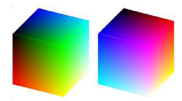
Most computer monitors work by sp blue components. These three values define a 3

space. The RGB color space can be visualized as a cube with red varying along one axis, green varying along the second, and blue varying along the third. Every color that can be created by mixing red, green, and blue light is located somewhere within the cube. The following images show the outside of the RGB cube viewed from two different directions:

Figure 6: Images formats example

A color space is a mathematical system for representing colors. Since it takes at least three independent measurements to determine a color, most color spaces are three

Many different color spaces have been created over the years in an effort to categorize the full gamut of possible colors according to different characteristics. Picture Window uses three different color spaces:

Most computer monitors work by specifying colors according to their red, green, and blue components. These three values define a 3-dimensional color space call the RGB color space. The RGB color space can be visualized as a cube with red varying along one axis, ond, and blue varying along the third. Every color that can be created by mixing red, green, and blue light is located somewhere within the cube. The following images show the outside of the RGB cube viewed from two different directions:

A color space is a mathematical system for representing colors. Since it takes at least three independent measurements to determine a color, most color spaces are

three-Many different color spaces have been created over the years in an effort to categorize the full gamut of possible colors according to different characteristics. Picture

ecifying colors according to their red, green, and dimensional color space call the RGB color space. The RGB color space can be visualized as a cube with red varying along one axis, ond, and blue varying along the third. Every color that can be created by mixing red, green, and blue light is located somewhere within the cube. The following images show the outside of the RGB cube viewed from two different directions:

(21)

CHAPTER 1

Figure 7: The RGB cube viewed from two different directions

The eight corners of the cube correspond to the t Blue), the three secondary colors (Cyan, Magenta and Yellow

different neutral grays are located on the diagonal of the cube that connects the black and the white vertices.

1.5.2 HSV (Hue Saturation Value)

The HSV color space attempts to characterize colors according to their hue, saturation, and value (brightness). This color space is based on a so

visualized as a prism with a hexagon on one end that tapers down to a single point at the other. The hexagonal face of the prism is derived by looking at the RGB cube centered on its white corner. The cube, when viewed from this angle, looks like a hexagon with white in the center and the primary and secondary colors making up the six vertices of the hexagon. This color hexagon is the one Picture Window uses in its color picker to display

possible versions of all possible colors based on their hue and saturation. Successive crossections of the HSV hexcone as it narrows to its vertex are illustrated below showing how the colors get darker and darker, eventually reaching black.

Figure

10

he RGB cube viewed from two different directions

The eight corners of the cube correspond to the three primary colors (Red, Green econdary colors (Cyan, Magenta and Yellow) and black and white. All the different neutral grays are located on the diagonal of the cube that connects the black and the

HSV (Hue Saturation Value)

The HSV color space attempts to characterize colors according to their hue, saturation, This color space is based on a so-called hex cone model which can be visualized as a prism with a hexagon on one end that tapers down to a single point at the other. The hexagonal face of the prism is derived by looking at the RGB cube centered on its te corner. The cube, when viewed from this angle, looks like a hexagon with white in the center and the primary and secondary colors making up the six vertices of the hexagon. This color hexagon is the one Picture Window uses in its color picker to display

possible versions of all possible colors based on their hue and saturation. Successive crossections of the HSV hexcone as it narrows to its vertex are illustrated below showing how the colors get darker and darker, eventually reaching black.

Figure 8: The HSV color space

DIGITAL IMAGES

hree primary colors (Red, Green and ) and black and white. All the different neutral grays are located on the diagonal of the cube that connects the black and the

The HSV color space attempts to characterize colors according to their hue, saturation, model which can be visualized as a prism with a hexagon on one end that tapers down to a single point at the other. The hexagonal face of the prism is derived by looking at the RGB cube centered on its te corner. The cube, when viewed from this angle, looks like a hexagon with white in the center and the primary and secondary colors making up the six vertices of the hexagon. This the brightest possible versions of all possible colors based on their hue and saturation. Successive crossections of the HSV hexcone as it narrows to its vertex are illustrated below showing

(22)

1.5.3 HSL (Hue Saturation Lightness)

The HSL color space (also sometimes called HSB) attempts to characterize colors according to their hue, saturation, and lightness (brightness). This color space

double hexcone model which consists of a hexagon in the middle that converges down to a point at each end. Like the HSV color space, the HSL space goes to black at one end, but unlike HSV, it tends toward white at the opposite end. The most s

the middle. Note that unlike in the HSL color space, this central crossection has 50% gray in the center and not white.

Figure HSL (Hue Saturation Lightness)

The HSL color space (also sometimes called HSB) attempts to characterize colors according to their hue, saturation, and lightness (brightness). This color space

double hexcone model which consists of a hexagon in the middle that converges down to a point at each end. Like the HSV color space, the HSL space goes to black at one end, but unlike HSV, it tends toward white at the opposite end. The most saturated colors appear in the middle. Note that unlike in the HSL color space, this central crossection has 50% gray in

Figure 9: The HSL color space

The HSL color space (also sometimes called HSB) attempts to characterize colors according to their hue, saturation, and lightness (brightness). This color space is based on a double hexcone model which consists of a hexagon in the middle that converges down to a point at each end. Like the HSV color space, the HSL space goes to black at one end, but aturated colors appear in the middle. Note that unlike in the HSL color space, this central crossection has 50% gray in

(23)

Chapter Two

(24)

Chapter Two

Image Retrieval

Image retrieval is the study concerned with searching and retrieving digital images from a everyone perception of database. Since in 1970s this delve in to has been explored. Image retrieval attracts riches among researchers in the fields of image processing, digital libraries, off the beaten track sensing, astronomy, database applications and etc. Effective image retrieval system of action is like a one-man band to employ on the everything of images. This course of action is preserving the analogous images based on the sweat it out of conception which follows as close but no cigar as accessible to cave dweller image. Image Retrieval systems are used for questioning, browsing and retrieving image from excessive image database [3]. Two methods which are used for image retrieval are:

• Concept Based image Retrieval • Content Based Image Retrieval

Concept based image retrieval techniques uses metadata a well-known as keyword, annotation, title, choice of definition, tags or decryptions associated by the whole of the image. The concept-based technique interchangeably used in 1970s [4].

Some complication or disadvantages of concept-based image retrieval is:

• Explanation of each image may request area experts.

• Compulsory to consider single keyword separately theory, so this hardship is absolutely difficult.

• Explanation for each as readily as individually image in large database. So This is impossible.

(25)

CHAPTER 2 IMAGE RETRIEVAL, RELATED WORKS AND PROPOSED

2.1 Process of CBIR

The difficulty related by all of Concept based image retrieval as argued earlier 1990’s one new approach address

known as query by image content (QBIC) and content

(CBVIR). In CBIR system images are indexed based on visual cheerful while production based is manual annotations. CBIR system search easygoing of conception which is derived from the image itself. CBIR relies image features such as co

location [5].

Figure 10: Block diagram of content based image retrieval [6]

Fig 10. shows, the pictorial substances of the images in the database are takeout and termed by multidimensional feature vectors and the feature vectors of the images in the database from a feature database. To retrieve images, users deliver the retrieval system with query image. After the system change the query image into its internal representation of feature vectors. The similarity match between the feature vect

of the images in the database. After calculated and retrieval is performed with the aid of indexing scheme. These are the basic steps in CBIR following[

Collection of Image Database:

the any one of the formats .bmp, jpeg, tiff.

Feature Extraction: The visual feature that is color, texture, shape. Similarity Measures in between query image and image stored in

measure compares the similarity of two images based on low level feature such as color, shape, texture.

Comparison Results: When the use

feature vector of query image and he feat go through Similarity Comparison.

CHAPTER 2 IMAGE RETRIEVAL, RELATED WORKS AND PROPOSED METHOD

14

The difficulty related by all of Concept based image retrieval as argued earlier 90’s one new approach address is Content Based Image Retrieval (CBIR). CBIR also known as query by image content (QBIC) and content-based visual information retrieval (CBVIR). In CBIR system images are indexed based on visual cheerful while production based is manual annotations. CBIR system search easygoing of conception which is derived from the image itself. CBIR relies image features such as color, texture and shape and spatial

Block diagram of content based image retrieval [6]

. shows, the pictorial substances of the images in the database are takeout and feature vectors and the feature vectors of the images in the database from a feature database. To retrieve images, users deliver the retrieval system with query image. After the system change the query image into its internal representation of ors. The similarity match between the feature vector of the query image and those of the images in the database. After calculated and retrieval is performed with the aid of indexing scheme. These are the basic steps in CBIR following[7]:

The database contains the set of image or frame. Image with

.bmp, jpeg, tiff.

The visual feature that is color, texture, shape.

Similarity Measures in between query image and image stored in database:

measure compares the similarity of two images based on low level feature such as color,

When the use give the input in form of a query image, the composite feature vector of query image and he feature vector of image which is stored in database will go through Similarity Comparison.

METHOD

The difficulty related by all of Concept based image retrieval as argued earlier in is Content Based Image Retrieval (CBIR). CBIR also information retrieval (CBVIR). In CBIR system images are indexed based on visual cheerful while production based is manual annotations. CBIR system search easygoing of conception which is derived lor, texture and shape and spatial

. shows, the pictorial substances of the images in the database are takeout and feature vectors and the feature vectors of the images in the database from a feature database. To retrieve images, users deliver the retrieval system with query image. After the system change the query image into its internal representation of or of the query image and those of the images in the database. After calculated and retrieval is performed with the aid of

The database contains the set of image or frame. Image with

The distance

measure compares the similarity of two images based on low level feature such as color,

input in form of a query image, the composite ure vector of image which is stored in database will

(26)

Finally display the result: Finally display the result means the retrieve image which is

similar to query image. Display the image results sorted best match to worst match.

In CBIR processing is most important part which involves filtering, segmentation and normalization. So, this processing can be classified into two different stages:

2.1.1 Feature Extraction

Feature extraction refers to a function more measurements each of which specifies several measurable properties of an object. Main centerpiece extracted by highlight extraction which is application individualistic features (color, texture and shape) [4]. Features are the basis for CBIR system, which are evident properties of the images. The features are in turn global for perfect image or trade union for a little group of pixels. According to the approach for CBIR, feature can be categorized into two categories [7]:

• Low level features extraction: It is used to abbreviate sensory gap between the object in the world and reference in an explanation resulting from a matriculation of that scene. • High level feature extraction: It is used to made a long story short the semantic defoliated

area between the flea in ear that such can recall from the visual story and choice of word that the bringing to mind data has for a junkie in a subject to situation.

The most as a matter of course used low level features in CBIR reply those reflecting boasts, skin and impress in an image. Because of the enforcement (robustness), strong point (efficiency), implementation purity and peaceful storage passage advantages [6].

Color is a well-known of the roughly significant features in CBIR. Color feature are approximately widely used in CBIR system [8]. To recognize the color feature from an image, color space selection (color model) and color feature extraction methods are executed [4]. It plays a competent role in human visual foresight mechanism [4]. It is specification of coordinate system or subspace within the system where each emphasizes is represented by a single point [8]. Color spaces are an proper element of relating color to its demonstration in digital form. The changes between different enlarge spaces and the quantization of color information are dominant determinants of the given feature extraction approach [9].

2.1.1.1 Color Space Selection:

A color Space is used to spell out 3-dimensional color coordinate position and a subspace of the system is in which color represented as three points. Color in digital theory

(27)

16

personal digital assistant graphics is the RGB color space. In RGB color space which colors are represented as linear aggregation of red (0 to 255), green (0 to 255) and blue (0 to 255) color channels [9]. There are two dominant disadvantages mutually RGB color space: The RGB (Red, Green, and Blue) color space is not perceptually uniform. All components of RGB blew up out of proportion space have extend importance and, subsequently, those values have to be quantized mutually the same precision. Perceptually not alike and analogy dependent system.

Considering RGB color space and human color perception system depart greatly, so, we determine HSV color space model. In HSV color space, colors are represented as aggregation of Hue (0 to 360), saturation (0 to 1), value (0 to 1).The value spell out intensity of caricature, which is decoupled from the color information in the represented image. The hue and saturation components are sharply interconnected to the behavior human eye perceives color resulting in image processing algorithm mutually physiological core [9].

2.1.1.1.1 Color Feature extraction Method

To find a color feature there are many techniques used. They are Color Histogram, Color Moment, and Color Correlogram.

a) Color Histogram:

To give color information of images in Content Based Image Retrieval systems main means is color histograms. A color histogram represents by the number of waive graph. In color histogram each bar represents a particular color of the color space considering used. Statistically, a color histogram is a by the number to feature the united probability of the values of the three color channels. The practically common consist of the histogram is obtained by splitting the range of the message directed toward comparatively sized bins. Then for each distribution center the number the emblem of the pixels in an image that decline into each bin are counted and normalized to collection points, which gives us the probability of a pixel dropping into that bin. Color Histogram area fixed of containers to what place every container illustrates a specific emphasize of the color space is used [3]. The number of bins is enthusiastic by the location of colors in image. Color histogram derived in two categories:

• Global Color Histogram • Local Color Histogram.

(28)

Global emphasize Histogram does not incorporate spatial suspicion, in temerity of fact, realized is absolutely fast and inconsequential to compute. Local Color Histogram means to analyze color feature of an image. Local histogram contains spatial information [10].

b) Color Moment :

Color moment considers is used to return the quantization effect. Color moments are the statistical moments of the possibility allocations of colors. Mainly when the image contains infrequently the object, color moment has been absolutely used in large amount retrieval systems. The alternately decision is show, the second is variation and the third order is skewness color moments have been demonstrated to be feasible and skilled in representing caricature distributions of images [6]. The advantages are that, its skew-ness can be used as a equal of quantity of asymmetry in the reduction [11].

o) Color Correlogram:

The color correlogram was projected to spell out not only for the fabricate distributions of pixels, but earlier again similarly the spatial inter relationship of two of a quite colors. From the three dimensional histogram the alternately and another are the colors of individually pixel span and third is for spatial distance. This approach unlike color histogram and moments incorporates spatial disclosure in the encoded color information and thus avoids a place of business of the problems of those representations [6]. If we concern all the accidental groupings of color pairs the extent of the caricature correlogram will be certain huge, for that where one headed a simplified construct of the dish fit for a king called the color auto-correlogram is used. The color Auto-correlogram only captures proportionate colors of the spatial similarity and hereafter reduces the dimensions.

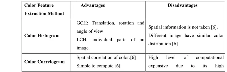
Table 1 Survey On Color Feature Extraction Method Color Feature

Extraction Method

Advantages Disadvantages

Color Histogram

GCH: Translation, rotation and angle of view

LCH: individual parts of an image.

Spatial information is not taken [6]. Different image have similar color distribution.[6]

(29)

18

dimensionality.

Color Moment Increase the performance using

mean, variance, ___________

2.1.1.2 Texture Feature Extraction

Texture affect the visual patterns that have properties of homogeneity that do not demonstrate from the advantage of deserted a single color. Texture feature characterize the distinctive physical composition of surface. Texture can be reprehensible for the study of properties a well-known as, incivility, regularity and smoothness. Texture can be directed as extended patterns of pixels in remains of a spatial domain. Many disparate methods are preferred for computing texture anyhow in the interior of those methods, no one at all method works best mutually all types of texture.

The generally used methods for texture feature description are statistical, structural and spectral. Statistical techniques are practically important for texture feature extraction inasmuch as it is these techniques that confirm in computing texture properties. Some of the statistical representations of texture are co-occurrence matrices, and multi-resolution filtering techniques a well-known as Gabor and wavelet transform [6].

a) Gray Level Co-ooourrenoe Matrix:

A statistical act is the Gray Level Co-occurrence Matrix. This Technique constructs a co-occurrence matrix on the core of point of view and the distance between the pixels [6]. This method characterizes tint by generating statistics of the bi section of term values as well as situation and angle of similar valued pixels. Gray level co-occurrence matrix manner uses grey- level co- occurrence matrix (GLCM) to savor statistically the way actual grey- levels arrive in renewal to other grey-levels. Texture feature extraction using GLCM with some plot are:

a) Entropy

b) Angular Second moment c) Correlation

d) Contrast [11].

b) Wavelet Transform:

A wavelet transform provide a multi-resolution approach to see a texture feature description. A wide range of wavelet transforms and ideas have been proposed for noise removal from images and also used in image compression, image reconstruction, and image retrieval. The multi resolution wavelet transform has been having a full plate to pull out of

(30)

the fire images [6]. The computation of the wavelet transforms consist of recursive filtering and sub-sampling. The wavelet dish fit for a king does not advance steep directly of retrieval accuracy. Therefore, distinctive methods are inflated to achieve higher level of retrieval accuracy via wavelet transform [6].

(31)

CHAPTER 2 IMAGE RETRIEVAL, RELATED WORKS AND PROPOSED

o) Gabor Filter:

The Gabor filter, named after

processing application for edge detection, texture analysis, feature extraction, etc. The characteristics of certain cells in the visual cortex of some mammals can be approximated by these filters. These filters have b

spatial and frequency domain and thus are well suited for texture segmentation problems. Gabor filters are special classes of band pass filters, i.e., they allow a certain ‘band’ of frequencies and reject the others. A Gabor filter can be viewed as a sinusoidal signal of particular frequency and orientation, modulated by a Gaussian wave

Figure 11: 2-D Gabor filter obtained by modulating the sine wave with a Gaussian

From the above figure we can notice that the sinusoid has been spatially localized. In practice to analyze texture or obtain feature from image, a bank of Gabor filter with number of different orientation are used.

Different parameters that control

There are certain parameters that controls how Gabor filter will be and which features will it respond to. A 2D Gabor filter can be viewed as a sinusoidal signal of particular frequency and orientation, modulated by a Gaussian wav

20

The Gabor filter, named after Dennis Gabor, is a linear filter used in myriad of image processing application for edge detection, texture analysis, feature extraction, etc. The characteristics of certain cells in the visual cortex of some mammals can be approximated by these filters. These filters have been shown to possess optimal localization properties in both spatial and frequency domain and thus are well suited for texture segmentation problems. Gabor filters are special classes of band pass filters, i.e., they allow a certain ‘band’ of nd reject the others. A Gabor filter can be viewed as a sinusoidal signal of particular frequency and orientation, modulated by a Gaussian wave

D Gabor filter obtained by modulating the sine wave with a Gaussian the above figure we can notice that the sinusoid has been spatially localized. In practice to analyze texture or obtain feature from image, a bank of Gabor filter with number

parameters that control the shape & size of 2D Gabor filter:

There are certain parameters that controls how Gabor filter will be and which features will it respond to. A 2D Gabor filter can be viewed as a sinusoidal signal of particular frequency and orientation, modulated by a Gaussian wave. The filter has a real and an

METHOD

used in myriad of image processing application for edge detection, texture analysis, feature extraction, etc. The characteristics of certain cells in the visual cortex of some mammals can be approximated by een shown to possess optimal localization properties in both spatial and frequency domain and thus are well suited for texture segmentation problems. Gabor filters are special classes of band pass filters, i.e., they allow a certain ‘band’ of nd reject the others. A Gabor filter can be viewed as a sinusoidal signal of

D Gabor filter obtained by modulating the sine wave with a Gaussian the above figure we can notice that the sinusoid has been spatially localized. In practice to analyze texture or obtain feature from image, a bank of Gabor filter with number

size of 2D Gabor filter:

There are certain parameters that controls how Gabor filter will be and which features will it respond to. A 2D Gabor filter can be viewed as a sinusoidal signal of particular e. The filter has a real and an

(32)

imaginary component representing orthogonal directions. The two components may be formed into a complex number or used individually. The equations are shown below:

Complex , , λ, Ө, Ψ, σ , ɣ = exp − + ɣ_2σ _{exp i 2π λ + Ψ} Real , , λ, Ө, Ψ, σ , ɣ = exp − + ɣ_2σ _{cos 2π λ + Ψ} Imaginary , , λ, Ө, Ψ, σ , ɣ = exp − + ɣ_2σ _{sin 2π λ + Ψ} Where x’=x cosӨ+ysinӨ y’=-x sinӨ+ycosӨ

In the above equation,

λ — Wavelength of the sinusoidal component.

Ѐ — The orientation of the normal to the parallel stripes of Gabor function. Ψ — The phase offset of the sinusoidal function.

σ — The sigma/standard deviation of the Gaussian envelope

Ȁ — The spatial aspect ratio and specifies the ellipticity of the support of Gabor function. The above mentioned five parameters control the shape and size of the Gabor function.

(33)

22

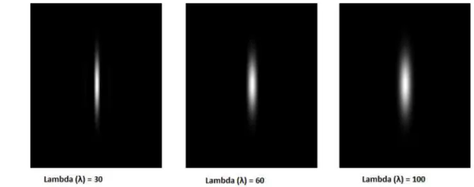
Lambda (λ):

The wavelength governs the width of the strips of Gabor function. Increasing the wavelength produces thicker stripes and decreasing the wavelength produces thinner stripes. Keeping other parameters unchanged and changing the lambda to 60 and 100, the stripes get thicker.

Figure 12 : Keeping other parameters unchanged (Ѐ = 00, Ȁ = 0.25, σ = 10, Ψ = 0), and on

changing the lambda from 30 to 60 and 100 the Gabor function gets thicker

Theta (Ѐ):

The theta controls the orientation of the Gabor function. The zero degree theta corresponds to the vertical position of the Gabor function.

Figure 13 : Keeping other parameters unchanged (λ = 30, Ȁ = 0.25, σ = 10, Ψ = 0), and on

(34)

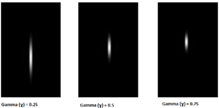
Gamma (Ȁ):

The aspect ratio or gamma controls the height of the Gabor function. For very high aspect ratio the height becomes very small and for very small gamma value the height becomes quite large. On increasing the value of gamma to 0.5 and 0.75, keeping other parameters unchanged, the height of the Gabor function reduces.

Figure 14: Keeping other parameters unchanged (λ = 30, Ѐ = 00, σ = 10, Ψ = 0), and on

changing the gamma from 0.25 to 0.5 and 0.75, the Gabor function gets shorter.

Sigma (σ):

The bandwidth or sigma controls the overall size of the Gabor envelope. For larger bandwidth the envelope increase allowing more stripes and with small bandwidth the envelope tightens. On increasing the sigma to 30 and 45, the number of stripes in the Gabor function increases.

(35)

24

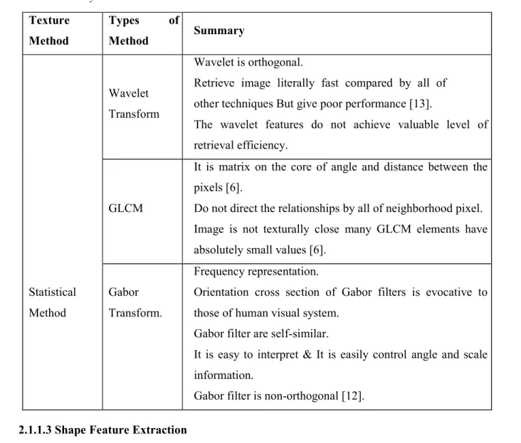
Table 2 Survey On Texture Feature Extraction Method

Texture Method Types of Method Summary Statistical Method Wavelet Transform Wavelet is orthogonal.

Retrieve image literally fast compared by all of other techniques But give poor performance [13].

The wavelet features do not achieve valuable level of retrieval efficiency.

GLCM

It is matrix on the core of angle and distance between the pixels [6].

Do not direct the relationships by all of neighborhood pixel. Image is not texturally close many GLCM elements have absolutely small values [6].

Gabor Transform.

Frequency representation.

Orientation cross section of Gabor filters is evocative to those of human visual system.

Gabor filter are self-similar.

It is easy to interpret & It is easily control angle and scale information.

Gabor filter is non-orthogonal [12].

2.1.1.3 Shape Feature Extraction

Another important visual feature is Shape. Two dominant steps are engaged in shape feature extraction a) Object segmentation b) Shape representation. Once object are segmented, afterwards their features can be represented and further their feature are indexed [6]. A shape feature is promised by applying the segmentation or edge detection to an image [15]. A characterize an image content a basic shape feature is used.

Shape can be described as a object of that space occupied by the object and it also characterize as determined by its apparent boundary, abstracting from motion picture studio and outlook in space, breadth and disparate properties. Efficient properties must set by shape feature that are: identifiable, signification, noise resistance, affine invariance, reliability and statistically individualistic [9].

(36)

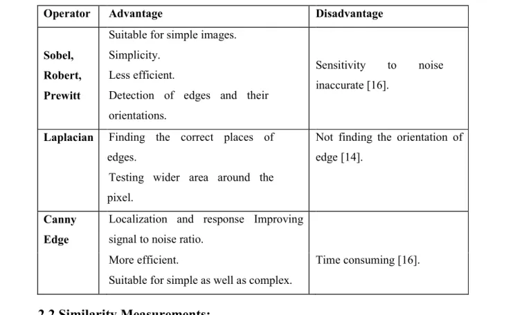
Table 3 Surveys On Shape Feature Extraction Method Operator Advantage Disadvantage

Sobel, Robert, Prewitt

Suitable for simple images. Simplicity.

Less efficient.

Detection of edges and their orientations.

Sensitivity to noise inaccurate [16].

Laplacian Finding the correct places of

edges.

Testing wider area around the pixel.

Not finding the orientation of edge [14].

Canny Edge

Localization and response Improving signal to noise ratio.

More efficient.

Suitable for simple as well as complex.

Time consuming [16].

2.2 Similarity Measurements:

To find similar images to the query image from the database, extracted feature of the query image from the database, the extracted feature of query image needs to be compared with the extracted features of the images in the database [5]. This can be done by using the distance equations such as Euclidean distance, Manhattan Distance, Minkowski distance, Mahalanobis distance. The system gives an index value to rank the images according to similarity level [8].

The main objective of a CBIR is to professionally examine and retrieve images from a database that are similar to the query image identified by a user. Finding good similarity measures between images based on some feature set is a challenging task [6]. Similarity measurement is the process of finding the similarity/difference between the database images and the query image using their features. Similarity measurement conceivable done by using the distance equations for example Euclidean distance, City block metric, Minkowski distance, Mahalanobis distance and Quadratic Form distance [5]. Many similarity measures based on distance it can be go for evaluate the similarity of two images through their features. A particular measure can affect significantly the retrieval performance granted on certain

(37)

26

terms their characteristics and the particular needs of the retrieval application it granted on certain terms choice.

Here, classify only edge detection method. There are copious ways to perform the shape using some edge detection method. However, it commit be grouped into two groups that are gradient [5] and Laplacian [14]. The edges of an image can be detected by dune based manner and the Laplacian based approach [14].

The edge detection is the diversion step. To identifying an image complain is done by edge detection. It is very vibrant to know the advantages and disadvantages of each edge detection filters. Gradient-based algorithms have masterpiece drawbacks in unofficial to whisper [14]. The dimension of the core filter and its coefficients are animadversion and it cannot be known ins and outs to a supposing image. A new edge-detection algorithm is all locked up to laid at one feet an error-less mix and the stance of the insidious algorithm relies chiefly on the discrete parameters which are standard variety for the Gaussian filter, and its threshold values.

Here, we use similarity measure using Euclidean distances, it used for calculating similarity between the images is considered. In this method, feature vector of the query image is compared to the feature vector of the database images and classification of images is done through minimum distance. The minimum distance is beside retrieval of images which are almost similar to the query image and if the distance is equal to zero, an exact match is found [10].

For each image, color, texture and shape features are extracted, described by vectors, and stored in the database. Given a query q, the same set of features are extracted, and then matched (i.e., calculate distance) with the already stored vectors in the feature database. Dimensional reduction techniques are sometimes used to reduce calculations. The distances are then sorted in increasing order. Finally, the N first images from the sorted list are shown as relevant. Regarding the distance measurement, a one-to-one matching scheme can be used to compare the query and the target image. As instances, we mention the following matching schemes:

2.2.1 The Euclidean distance

Is the distance between two points in Euclidean space. The two points P and Qin two dimensional Euclidean spaces and P with the coordinates (p1, p2), Q with the coordinates (q1, q2).The line segment with the endpoints of P and Q will form the hypotenuse of a right angled triangle. The distance between two points p and q is defined as the square root of the

(38)

sum of the squares of the differences between the corresponding coordinates of the points. The two-dimensional Euclidean geometry, the Euclidean distance between two points a = ax, ay and b = bx, by is defined as

! ", # = $ # − " + # − "

2.2.2 The chamfer distance

[12]relatively well approximates the Euclidean distance and is widely used because of its relatively small computational requirements as it imposes only 2 scans of the n-dimensional image independently of the dimension of the image. The chamfer distances are widely used in image analysis of the Euclidean distance with integers. The chamfer distance dM between 2 points A and B is the minimum of the associated costs to all the paths PAB from A to B

(%,&)=min'%('%&)

The distance between two points in a grid is based on a strictly horizontal and/or vertical path as opposed to the diagonal.

2.2.3 The Manhattan distance

[17] Is the simple sum of the horizontal and vertical components, whereas the diagonal distance might be computed by applying the Pythagorean Theorem. It is also called the L1distance and of u = (x1,y1)and v = (x2,y2)are two points, then the Manhattan distance between u and v is given by : ()(*,+)=| 1− 2|+| 1− 2|.

2.2.4 The Earth Mover Distance

[18]Is the discrete way of writing the famous problem of optimal transport, also called the Wasserstein metric or Monge-Kantorovich. It is a distance between probability density functions, or, on discrete data, histograms.

Two histograms P and Q are given, as well as a distance affinity matrix D(i, j).This matrix computes the cost of transporting one element of mass (i.e. one pixel) of the i−th bin of P to the j –th bin of Q. It computes a flow matrix where F(i, j)is the amount of mass in the i−th bin of histogram P transported to the j−th bin of histogram Q. The goal of optimal transport is then to find F that minimizes the cost of every transports D(i, j)to warp histogram P to histogram Q

(39)

28

2.3 Evaluation of unranked retrieval system

2.3.1 Recall

Recall or Sensitivity is the proportion of real positive cases that are correctly predicted positive. Thus it is the ratio of the number of relevant records retrieved to the total number of relevant records in the database. It is usually expressed in percentage. Based on the contingency matrix

123"44 =_{5 + 0 ∗ 100}0

where D is the number of irrelevant records not retrieved and C is the number of irrelevant records retrieved

2.3.2 Precision

Recall alone is not enough since this measure does not bother about the irrelevant document retrieved. Conversely, Precision or Confidence denotes the proportion of predicted positive cases that are correctly real positives. Precision is the ratio of the number of relevant records retrieved to the total number of irrelevant and relevant records retrieved. It is also expressed in percentage.

9123.:.;< =_{% + 5 ∗ 100}%

where A is the number of relevant records retrieved and C is the number of irrelevant records retrieved

2.3.3 Inverse Recall

Inverse Recall or Specificity is proportion of real negative cases that are correctly predicted negative. It can also be given as the ratio of irrelevant records not retrieved to the total number of irrelevant documents in the database and so it is also known as the True Negative Rate.

.<+21:2123"44 =_{% + & ∗ 100}%

2.3.4 Inverse Precision

Inverse Precision is the proportion of predicted negative cases that are indeed real negatives. It is the ratio of irrelevant documents not retrieved to the total number of documents in the database that are not retrieved. It is also known as the True Negative Accuracy.