Analysis of SMOS sea surface salinity data using DINEOF

Analysis of SMOS sea surface salinity data using DINEOF

Aida Alvera-Azcárate

⁎

_{, Alexander Barth}

_{, Gaëlle Parard}

_{, Jean-Marie Beckers}

a

AGO-GHER-MARE, University of Liège, Allée du Six Aout, 17, Sart Tilman, Liège 4000, Belgium

b_{F.R.S.-FNRS (National Fund for Scientific Research), Brussels, Belgium}

a b s t r a c t

a r t i c l e i n f o

Article history: Received 31 July 2015

Received in revised form 23 December 2015 Accepted 18 February 2016

Available online 28 February 2016

An analysis of daily Sea Surface Salinity (SSS) at 0.15 °×0.15° spatial resolution from the Soil Moisture and Ocean Salinity (SMOS) satellite mission using DINEOF (Data Interpolating Empirical Orthogonal Functions) is presented. DINEOF allows reconstructing missing data using a truncated EOF basis, while reducing the amount of noise and errors in geophysical datasets. This work represents afirst application of DINEOF to SMOS SSS. Results show that a reduction of the error and the amount of noise is obtained in the DINEOF SSS data compared to the initial SMOS SSS data. Errors associated to the edge of the swath are detected in 2 EOFs and effectively removed from thefinal data, avoiding removing the data at the edges of the swath in the initial dataset. Thefinal dataset presents a cen-tered root mean square error of 0.2 in open waters when comparing with thermosalinograph data at their orig-inal spatial and temporal resolution. Constant biases present near land masses, large scale biases and latitudorig-inal biases cannot be corrected with DINEOF because persistent signals are retained in high order EOFs, and therefore these need to be corrected separately. The signature of the Douro and Gironde rivers is detected in the DINEOF SSS. The minimum SSS observed in the Gironde plume corresponds to aflood event in June 2013, and the shape and size of the Douro river shows a good agreement with chlorophyll-a satellite data. These examples show the capacity of DINEOF to remove noise and provide a full SSS dataset at a high temporal and spatial reso-lution with reduced error, and the possibility to retrieve physical signals in zones with high initial errors.

© 2016 Elsevier Inc. All rights reserved.

1. Introduction

Sea Surface Salinity (SSS) is being measured globally by the Soil Moisture and Ocean Salinity (SMOS) satellite mission, allowing obtaining an unprecedented spatial and temporal coverage in the mea-surement of this variable. SMOS measures radio frequency emission in thefirst centimeters of the upper ocean. The SMOS salinity mission has a target accuracy of ~ 0.2 over 100 km2_{and 30 days (Lagerloef &} Font, 2010). Salinity is derived through the relation between brightness temperature (BT), sea surface temperature (SST) and sea roughness. This relation is more reliable for high values of BT and SST, so the preci-sion of the salinity estimates decreases at high latitudes. Other sources of error for remotely-sensed SSS are sea roughness, astronomical radia-tion sources (e.g. galactic glint and cosmic background), sun glint, atmo-sphere attenuation of the emitted signal and proximity to land and ice (Lagerloef, Schmitt, Schanze, & Kao, 2010; Boutin et al., 2012). In addi-tion, illegal anthropic radio emissions (radio-frequency interference, RFI) in the protected L-band frequency result in permanently or inter-mittently contaminated zones of the ocean, such as the European seas and Asia (Boutin et al., 2012). These sources of error result in noise and biases that need to be corrected, and gaps in the satellite SSSfields.

Several features have been analyzed using SMOS SSS data, showing the importance of this dataset. For example, the North Atlantic subtrop-ical salinity maximum (Kolodziejczyk, Hernandez, Boutin, & Reverdin, 2015), the Gulf Stream meanders (Reul et al., 2014), and the Amazon river plume (Grodsky, Reverdin, Carton, & Coles, 2014; Reul et al., 2014; Fournier, Chapron, Salisbury, Vandemark, & Reul, 2015). Process-es at smaller scalProcess-es, or featurProcess-es near land massProcess-es are more difficult to analyze using SMOS SSS because of the systematic errors due to the proximity of land.

DINEOF (Data Interpolating Empirical Orthogonal Functions) is a technique to reconstruct missing data in geophysical datasets that uses a truncated EOF basis in an iterative approach. DINEOF has been successfully applied to sea surface temperature (e.g.Alvera-Azcárate, Barth, Rixen, & Beckers, 2005), chlorophyll-a and winds (e.g. Alvera-Azcárate, Barth, Beckers, & Weisberg, 2007), and total suspended matter (e.g.Sirjacobs et al., 2011; Alvera-Azcárate, Vanhellemont, Ruddick, Barth, & Beckers, 2015). This work represents thefirst attempt at using DINEOF with salinity data. The challenges faced in the use of DINEOF to analyze SSS are the high level of noise in the SMOS SSS data, the presence of constant biases and errors due for example to the presence of land masses, and the lack of knowledge about the spatial and temporal signatures in SSS and how to separate them from the mentioned errors. Constant biases cannot be corrected with DINEOF so these should be removed separately, using for example the approach suggested byKolodziejczyk et al. (2016-in this issue).

⁎ Corresponding author.

E-mail address:a.alvera@ulg.ac.be(A. Alvera-Azcárate).

http://dx.doi.org/10.1016/j.rse.2016.02.044 0034-4257/© 2016 Elsevier Inc. All rights reserved.

Contents lists available atScienceDirect

Remote Sensing of Environment

The aim of this work is to assess if DINEOF is able to detect and re-move noise and errors from the SMOS SSS dataset at the highest tempo-ral and spatial resolution provided by the data. By removing noise and errors at the highest resolution, these data do not enter into the compu-tation of composites and can provide therefore improved estimates at 10-day or monthly averages.

This work is organized as follows: the satellite and in situ data used are described inSection 2.Section 3describes the methods used in this work: pre-processing of the data, and a description of DINEOF and the outlier detection methodology. The results section consists of a sensitiv-ity study, a comparison with independent data, an assessment of the spatial resolution achieved by the data, the analysis of thefinal dataset and the description of the EOF basis used for the computation of the final dataset. These are presented inSection 4. We conclude this work inSection 5.

2. Data used 2.1. Satellite data

Level 2 Ocean Salinity User Data Product (UDP) version 5.50, provid-ed by ESA, are usprovid-ed in this study. The domain coverprovid-ed is the North-East Atlantic Ocean and Mediterranean Sea, as shown inFig. 1. Daily data for 2013 consisting of the ascending orbits have been selected, and the SSS data calculated using Roughness Model 1 (Yin, Boutin, Martin, & Spurgeon, 2012) have been retained for this study. Only ascending or-bits are used to avoid working with data that have a different accuracy, as the descending orbits present larger errors than the ascending orbits. The data are kept at the original spatial resolution, which is of 0.15 ° × 0.15°. Data located farther than ± 300 km of the centre of the track are subject to higher errors (Zine et al., 2008; Yin et al., 2014), and are therefore typically removed (i.e.Boutin et al., 2014). In this work, however, we have retained the full swath in order to assess if these errors at the edges of the swath can be discarded through the DINEOF analysis. Mediterranean Sea data are also subject to large errors, but the data are retained as well in this work in order to assess if DINEOF is able to extract a physically meaningful signal from the initial SSS.

For a qualitative assessment of the salinity data near the river plume of the Douro river we use 8-day composites of MODIS (Moderate Reso-lution Imaging Spectroradiometer) Aqua level 3 chlorophyll-a data, with a spatial resolution of 4 km and obtained fromhttp://oceancolor. gsfc.nasa.gov/.

2.2. In situ data

In situ salinity data for 2013 have been extracted from the World Ocean Database (WOD) 2013 (Boyer et al., 2013),http://www.nodc. noaa.gov/and the Coriolis Data Centre (http://www.coriolis.eu.org/). Data from all platforms are extracted (Argo, CTD, drifting buoys and moored buoys), and the shallowest value is retained for each profile (with a maximum depth of 2 m). Note that most Argo data stop measur-ing when reachmeasur-ing depths shallower than 5 m, therefore most of the data used here have an effective depth that is deeper than 2 m. The in situ data have been randomly distributed into a training dataset (90% of the data) and a validation dataset (10% of the data). The training dataset has been used to compute a monthly climatology using divand (n-dimensional Data Interpolating Variational Analysis,Barth et al. (2014)). This technique is equivalent to DIVA (Troupin et al., 2012) but multi-dimensional analyses can be handled, which allows taking into account for example the temporal correlation existing in the data. A SSSfield has been calculated for each month of 2013, with a spatial resolution of 0.5 degrees. The spatial correlation length has been established to 10 degrees for thefirst guess and 1 degree for the short-scale background. The temporal correlation length is 90 days for thefirst guess and 15 days for the short-scale background. Signal-to-noise ratio is set up to 20. The spatial and temporal correlation scales have been optimized by minimizing the RMS between the analysis and a cross-validation dataset consisting of 5% of the initial data chosen at random. Signal-to-noise ratio was optimized by the same procedure. These monthlyfields, interpolated to daily values, are removed from the SMOS SSSfields prior to the DINEOF analyses in order to work with anomalies, and an example for February, July and December is shown inFig. 2. Evidently, the presence of features like the Gulf Stream or the subtropical salinity maximum in the background fields depends

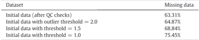
Fig. 1. Percentage of missing data of the SSS data after quality checks and outlier detection. Top panel: spatial distribution of the percentage of missing data. The green circle marks the position of the Douro river mouth, and the red triangle marks the position of the Gironde estuary. Bottom panel: temporal evolution of the percentage of missing data.

strongly on the presence of enough data to resolve them, as in the case of the Gulf Stream weaker amplitude in February (top panel ofFig. 2). The validation dataset (10% of the initial data, not used in the back-ground) is used in the comparison with the original SSS and DINEOF re-construction, inSection 4.

Thermosalinograph (TSG) data from Voluntary Observing Ships dis-tributed by Legoshttp://www.legos.obs-mip.frare also used in this work for comparison purposes. The TSG SSS data are measured every 5 min over a series offixed tracks along the North Atlantic Ocean and the Mediterranean Sea.

3. Methods

3.1. Data pre-processing

Several qualityflags, provided with the original data, are used in order to remove data suspected of low quality. These are the_{flag for} poor geophysical retrieval Fg_ctrl_poor_geophysical (which detects sun glint, galactic glint, wind speed and suspected ice), theflag for poor retrieval Fg_ctrl_poor_retrieval (bad convergence of the algorithm calculating SSS) and a qualityflag specific for the roughness model used (Dg_quality_SSS1). A pixel with the threeflags activated is removed from the dataset. While this qualityflag setup is likely to allow pixels with a bad quality to be retained, the aim of this work is tofilter these bad data in later steps with the DINEOF processing.

Two additional steps are performed in order to remove data with low quality. Thefirst one consists of a range check in which pixels with a value too high or too low with respect to the monthly climatolo-gy calculated using the data described inSection 2.2are removed. This test is performed on a pixel basis, and the difference threshold is set to ± 2. Finally, the outlier detection procedure described inSection 3.3, based on DINEOF, is applied. The parameters used for the outlier detec-tion have been determined through a sensitivity analysis which will be shown inSection 4.1.

Thefinal dataset has an average amount of missing data of 75.45%, and the average percentage of missing data in space and time is shown inFig. 1. The highest amount of missing data (more than 90%) is found in the eastern part of the North Atlantic Ocean and the

Mediterranean Sea. Part of the eastern Mediterranean Sea does not con-tain any data after the quality checks (white areas inFig. 1), and there-fore these zones are not used in the rest of this work. The percentage of missing data is the lowest in September, and while it is difficult to deter-mine the reason for this decrease in the percentage of missing data, a possible cause is that during this period of the year both temperature and salinity reach their highest values in the zone of study, which might result in a lower signal-to-noise ratio in the calculation of SSS, and therefore to more data passing the quality checks.

3.2. DINEOF

DINEOF (Data Empirical Orthogonal Functions,Beckers and Rixen (2003),Alvera-Azcárate et al. (2005)) has been used in this study in order to calculate daily SSSfields with low noise and reduced error. DINEOF consists of an EOF-based reconstruction of the missing data in a geophysical dataset, extracting the main patterns of variability from the data. It uses a truncated EOF basis to infer the missing data, and therefore noise can be effectively reduced in the reconstructed dataset, as noise is typically found in the higher order EOFs. Some transient in-formation, however, can be also removed from thefinal result as these might be also found in the higher order EOFs. In order to calculate the EOF basis from a dataset that has missing data, the following steps are performed:first the monthly climatology described inSection 2.2 (in-terpolated to daily values) is removed from the data, and the missing values are set to zero (i.e. the mean of the dataset). Afirst EOF decompo-sition using only thefirst EOF is performed, and this reduced EOF basis is used to infer an improved estimation of the missing data. Once conver-gence has been reached for the estimation of the missing data using the first EOF, the whole procedure is repeated using 2 EOFs. Then 3, 4… n EOFs are calculated. The total number of EOFs to be calculated, n, is de-termined by cross-validation: a set of initially valid data (about 3% of the total data) is set aside at the beginning and treated as missing data. At each step, a cross-validation error is calculated. The number of EOFs that minimizes this error is used as the optimal for the dataset recon-struction. More details about DINEOF and examples can be found in

Beckers and Rixen (2003),Alvera-Azcárate et al. (2007, 2005). Afilter was applied to the temporal covariance matrix, based in

Alvera-Azcárate, Barth, Sirjacobs, and Beckers (2009). Thisfilter was ini-tially implemented to improve the temporal sequence of the analyzed images. In case of large amounts of missing data (Alvera-Azcárate et al., 2009), or highly irregular time steps (Alvera-Azcárate et al., 2015), thefilter allows improving the reconstruction by taking into ac-count the temporal coherency of the data. In this case, the aim was to smooth the reconstruction and improve the temporal coherence of the data, as the percentage of missing data is very high in certain zones, which results in not enough data to perform a DINEOF reconstruction if nofilter is used. In order to test the effect of this filter in the final qual-ity of the data, twofilter lengths are presented in the sensitivity study of

Section 4.1. 3.3. Outlier detection

In order to detect outliers in the initial SSS dataset, before performing thefinal analysis using DINEOF, an outlier detection proce-dure consisting of three tests is applied to the data, following Alvera-Azcárate, Sirjacobs, Barth, and Beckers (2012). In thefirst test (“EOF test”) suspect data are detected as those presenting a large residual with respect to a truncated EOF basis calculated using DINEOF. The sec-ond test (“Median test”) aims to detect departures from a local median (calculated in a 20 by 20 pixel box) and the third test (“Proximity test”) penalizes more strongly pixels in the vicinity of land or missing data (e.g. at the edges of the swath, or near other pixels already classified as bad by the qualityflags). A weighted combination of these three tests is performed (in this study, an equal weight of 1/3 is given to all tests), andfinally a threshold to classify a given pixel as an outlier is

Fig. 2. Example of monthly background SSSfields calculated using in situ data. Top panel: in situ SSS for February 2013; middle panel: in situ SSS for July 2013; bottom panel: in situ SSS for December 2013.

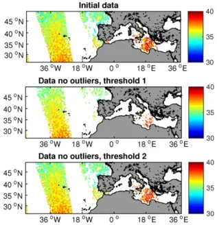
decided.Fig. 3shows an example of the three outlier detection sub-tests for 7 February 2013. The effect of thefinal threshold in the quantity of eliminated data is shown inFig. 4for 7 February 2013 as well, where two thresholds are shown: 1 (stronger, i.e. more data are classified as outliers) and 2 (weaker). As expected, a higher concentration of outlier data is found at the edges of the swaths, near land and in the Mediterra-nean Sea. The initial SSSfield and the resulting fields when applying the outlier detection with the two mentioned thresholds are shown in

Fig. 5. The weights given to each sub-test and thefinal threshold depend on the initial data quality and thefinal use of the data. In this work the final threshold is set to one, which eliminates 12.14% of data (seeTable 1

to see the impact of the outlier threshold in the amount of missing data). For more details and examples using other variables (sea surface tem-perature and chlorophyll-a concentration) the readers are referred to

Alvera-Azcárate et al. (2012). 4. Results

4.1. Sensitivity study

Once the SSS data have been checked for their quality and the out-liers have been removed, a DINEOF analysis is performed in order to ob-tain full SSSfields at daily temporal resolution and 0.15°×0.15° spatial resolution. In order to determine the optimal values for the temporal co-variancefilter and the outlier threshold, a series of analyses have been realized with varying values for these parameters. Regarding the length of the temporal covariancefilter, two values are shown here: 3 and 14 days, representing a short and a longfilter. Other tests were done with intermediate values that are not shown here. The 14-dayfilter, as shown in the following, provided better results than any of the other testedfilter lengths. The repeat cycle of SMOS is 18 days, but, as ad-dressed later inSection 4.5, using a 18-day length for the temporal covariancefilter results in part of the signal considered erroneous being retained in the EOF basis, and therefore we chose 14 days as the maximumfilter length in this work. The reader is cautioned howev-er that the optimalfilter length will vary from one dataset to another, and therefore an optimisation of this value must be realized for each dataset. A summary of the number of EOFs retained by the DINEOF

reconstruction, the variance explained and the cross-validation error obtained is included inTable 2.

Using a very short temporal covariancefilter length (3 days) results in a reconstruction using one EOF, while the three reconstructions test-ed using a longerfilter (14 days) results in reconstructions using 5 EOFs. The number of EOFs has an effect in the quantity of explained variance, and therefore in the quality of thefinal reconstruction. For this case, it therefore appears that longerfilter lengths provide better results, with the reconstruction using an outlier threshold of 1 retaining the highest variance (78%, seeTable 2).

In order to establish the impact of the different parameters used, a comparison of each reconstruction with the in situ validation dataset and the TSG data described inSection 2.2has been realized. The results of this comparison are summarized inTable 3. It can be seen that, in gen-eral, the choice of the outlier threshold level has a strong influence in the quality of thefinal result: for example, the centered RMS error of the DINEOF reconstructed data when compared with TSG data is of 0.6 for afilter length of 14 days and outlier threshold of 2, and this value decreases to 0.55 when the outlier threshold is 1. For afilter length

Fig. 3. Example of the three sub-tests for the detection of outliers for 7 February 2013. Top panel: EOF test (unitless, larger values mean larger departures from the EOF basis). Middle panel: proximity test (unitless; a value of 3 is assigned to pixels near land or missing data, zero value for the rest). Bottom panel: median test (unitless, larger values mean larger departures from the local median).

Fig. 4. Example of the data classified as outliers for 7 February 2013, using two thresholds: 1 (top panel) and 2 (bottom panel). The total number of outliers detected for each threshold is given in the title of each sub-figure.

Fig. 5. Top panel: initial SSS data (after quality checks) for 7 February 2013. Middle panel: initial data with outliers removed, using a threshold of 1. Bottom panel: initial data with outliers removed, using a threshold of 2.

of 3 days and an outlier threshold of 1, the centered RMS decreases fur-ther to 0.49. Similar reductions are observed in the comparison with WOD and Coriolis data, although the number of match-ups is very low. These results lead to the conclusion that an outlier threshold of 1 is the best choice. Regarding thefilter length, it appears that the short filter value (i.e. 3 days) leads to improved results, although as it has been shown inTable 2, this reconstruction uses only one EOF, which de-creases the explained variance and results in a smoother reconstruction which may explain the lower error values. Large fresh biases are observed in all comparisons. As mentioned before, DINEOF is not able to remove constant or persistent biases from the initial data. As a con-clusion of the sensitivity study, the results of the reconstruction using afilter length of 14 days and an outlier threshold of 1 will be used in the remaining of this work.

4.2. Comparison with TSG data

The comparison with TSG data inTable 3reveals that the fresh bias ob-served in the initial data (_{−0.39) increases to −0.57 in the} reconstruc-tion provided by DINEOF (Table 3). In order to assess the causes of this increase, the comparison between TSG and SMOS data will be looked at with more detail.Fig. 6shows the TSG data and the SMOS data (anomaly with respect to the TSG data) at the TSG positions. The DINEOF data along the French, Spanish and Portuguese coasts present the lowest values with respect to the TSG data. These data are not present in the original SMOS data, and therefore the bias of the original SMOS data appears -artificially- to be lower than the DINEOF reconstruction. Large biases in SMOS SSS can be expected near land due to land contamination issues. Latitudinal or large scale bias is also present in the original data, and as mentioned before DINEOF does not aim at correcting these sources of bias.Fig. 6also includes the DINEOF estimate at the initially present SMOS positions, showing the ability of DINEOF to reduce noise in the data.

Fig. 7shows a scatter plot comparing the initial SMOS data and DINEOF data (at positions initially present in SMOS and at all points), with the color representing the longitude of the data. It can be seen that the DINEOF results at positions initially present in SMOS are much closer to the 1:1 line than the original SMOS data. When looking at the DINEOF results at all points we can see that data at around 10°W depart largely from the 1:1 line, and these are again the data near the French, Spanish and Portuguese coasts. The DINEOF SSS data at the Mediterranean Sea (in deep red inFig. 7, longitudes larger than 0°E) do present also a slightly larger bias than the average data, but this bias is smaller than the one along the French, Spanish and Portuguese coasts in the North Atlantic Ocean.

It should also be noted that the error statistics ofTable 3include zones that are very close to land and the Mediterranean Sea, which are typically not available in other SMOS SSS products, and therefore not used in comparisons with in situ data. A comparison using only DINEOF SSS data at open ocean locations (west of 24∘W) reveals a cen-tered RMS of 0.61 when comparing to WOD and Coriolis data and of 0.32 when comparing to TSG data (Table 4), a reduction of 40% with re-spect to the error of the initial SMOS data.

4.3. Spatial resolution of the reconstruction

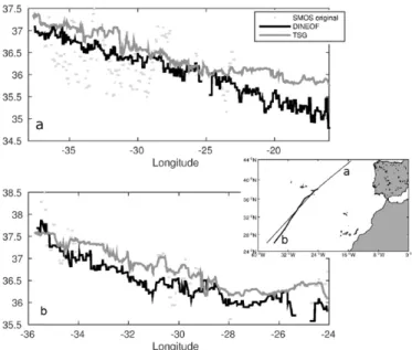
In order to show the effective spatial resolution that the DINEOF re-construction is able to retain, two transects of TSG data are compared to the SMOS data at very high spatial resolution. Co-located transects of TSG salinity, SMOS and DINEOF SSS are shown inFig. 8. The TSG data

Table 1

Percentage of missing data in the initial SMOS SSS dataset (after the quality checks de-scribed inSection 2.1) and after the outlier detection tests, using 3 thresholds.

Dataset Missing data

Initial data (after QC checks) 63.31% Initial data with outlier threshold = 2.0 64.87% Initial data with threshold = 1.5 68.84% Initial data with threshold = 1.0 75.45%

Table 2

Number of EOFs retained by DINEOF, percentage of explained variance and cross-valida-tion error for analyses using different values of the covariancefilter length and outlier threshold.

# EOFs Variance explained

Cross-validation error Filter length Outlier threshold

3 1 1 64% 0.76

14 1 5 78% 0.75

14 1.5 5 71% 0.76

14 2 5 68% 0.75

Table 3

Comparison statistics between in situ data and SMOS data for twofilter lengths (3 days and 14 days) and two outlier threshold levels (1.0 and 1.5). The two in situ datasets used (WOD/Coriolis and thermosalinograph data) are described in the text. The DINEOF recon-struction is compared at initially present points and at all available points. Statistics used are Root Mean Square Error (RMS), centered RMS (CRMS), bias and Correlation (r). The number of data used for each calculation is included. Note the low number of data avail-able for some of the comparisons using initial SMOS data.

RMS CRMS Bias r # data Filter length 3 days

Outlier threshold 1.0

WOD/Coriolis initial 0.85 0.76 −0.37 0.33 11 WOD/Coriolis DINEOF initial points 0.36 0.31 −0.18 0.82 11 WOD/Coriolis DINEOF 0.55 0.54 −0.1 0.79 1557 TSG initial 0.67 0.55 −0.4 0.79 29 TSG DINEOF initial points 0.42 0.33 −0.26 0.89 29 TSG DINEOF 0.71 0.49 −0.52 0.88 184 Filter length 14 days

Outlier threshold 1.0

WOD/Coriolis initial 0.71 0.7 −0.1 0.7 8 WOD/Coriolis DINEOF initial points 0.43 0.41 −0.14 0.76 8 WOD/Coriolis DINEOF 0.67 0.64 −0.2 0.72 1557 TSG initial 0.67 0.55 −0.39 0.79 29 TSG DINEOF initial points 0.53 0.37 −0.38 0.87 29 TSG DINEOF 0.79 0.55 −0.57 0.86 184 Outlier threshold 1.5

WOD/Coriolis initial 0.64 0.6 −0.24 0.5 26 WOD/Coriolis DINEOF initial points 0.52 0.49 −0.17 0.78 26 WOD/Coriolis DINEOF 0.68 0.64 −0.2 0.72 1567 TSG initial 0.73 0.6 −0.43 0.77 38 TSG DINEOF initial points 0.56 0.35 −0.4 0.92 38 TSG DINEOF 0.86 0.57 −0.64 0.85 184 Outlier threshold 2

WOD/Coriolis initial 0.77 0.67 −0.37 0.67 49 WOD/Coriolis DINEOF initial points 0.61 0.58 −0.19 0.56 49 WOD/Coriolis DINEOF 0.72 0.67 −0.27 0.7 1568 TSG initial 0.87 0.70 −0.51 0.73 44 TSG DINEOF initial points 0.61 0.4 −0.47 0.90 44 TSG DINEOF 0.92 0.6 −0.7 0.84 184

Table 4

Comparison statistics between in situ data and SMOS data for open waters (longitudes west of 24°W), for afilter length of 14 days and an outlier threshold of 1. There are not enough match-up points to assess the error between SMOS data and WOD. Statistics used are Root Mean Square Error (RMS), centered RMS (CRMS), bias and Correlation (r). The number of data used for each calculation is included. Note the low number of data avail-able for some of the comparisons using initial SMOS data.

RMS CRMS Bias r # data WOD/Coriolis initial – – – – – WOD/Coriolis DINEOF initial points – – – – – WOD/Coriolis DINEOF 0.62 0.61 −0.12 0.67 1372 TSG initial 0.59 0.53 −0.25 0.66 20 TSG DINEOF initial points 0.28 0.19 −0.2 0.91 20 TSG DINEOF 0.39 0.32 −0.22 0.94 48

are kept at their original temporal resolution (~5 min) in order to show the capability of the DINEOF SSS to reproduce small-scale variations. The original and DINEOF SSS data (daily data at 0.15° × 0.15°) are inter-polated to the TSG positions. Two transects are shown, one getting closer to the European coasts. It is observed that DINEOF is able to strongly reduce the noise in SMOS data, and at the same time reproduce the small-scale variations observed in the TSG data. There is a constant fresh bias in the DINEOF data, that increases when getting close to the coast (east of 24°W). The centered RMS for transect a is 0.22 and the bias is−0.35. For transect b, which is located only in open ocean, the centered RMS is 0.2 and the bias is−0.3. These results show the capa-bility of DINEOF to retain the high resolution of the initial dataset. 4.4. Reconstruction results

An example of the reconstructed SSS provided by DINEOF is shown inFig. 9for 21 July 2013. This example shows the capability of DINEOF to reduce the noise still present in the daily SSSfields after the quality checks and the outlier check performed in this work. The Gulf Stream is well observed in the top left part of the domain, with fresher waters and meanders of about 200 km in size. Two low salinity zones around the Gironde (France) and the Douro (Portugal) rivers are also observed, indicating that these river plumes can as well have a signature in the SMOS SSS maps, once the appropriate corrections have been applied. Large river plumes have already been studied using SMOS data (e.g. the Amazon river plume, Grodsky et al., 2014; Reul et al., 2014; Fournier et al., 2015), but the Douro and Gironde river plumes, because of their smaller size and the large biases caused by land contamination, have not yet been assessed using SMOS data. Although it is difficult to assess quantitatively the accuracy of the SMOS data at these river

plumes, the qualitative description of these signals can be helpful to an-alyze the extent of the plumes and their seasonal variability.

Fig. 10presents the averaged salinity time series at the Douro and Gironde river plumes along 2013 (the boxes delimiting these two zones are shown inFig. 9). The Douro river plume shows values ranging from 33 to 35.4. The Gironde plume shows values ranging from 32.2 to 33.7, with minimum values in June and November 2013. Following

Jalón-Rojas, Schmidt, and Sottolichio (2015), aflood event occurred in

Fig. 6. First panel: TSG data, averaged daily. Second panel: original SMOS SSS data anomalies with respect to the TSG data. Third panel: DINEOF reconstruction of SSS data (anomalies with respect to the TSG data) at the initially present SMOS positions. Fourth panel: DINEOF reconstruction of SSS data anomalies with respect to the TSG data at all positions. Fresh biases can be seen along the French, Spanish and Portuguese coasts.

Fig. 7. Scatter plots comparing the SMOS data and DINEOF reconstruction to TSG data. Top panel: SMOS data vs. TSG data. Middle panel: DINEOF reconstruction at originally present points vs. TSG data. Bottom panel: DINEOF reconstruction at all points vs. TSG data. The colors indicate the longitude of each point in the graphic.

the Gironde estuary in June 2013 (see theirFig. 3), which explains the low salinity values observed in the DINEOF reconstruction. This mini-mum in the DINEOF SSS is observed to develop quickly at the beginning of June, and erode during July (data not shown). The minimum SSS ob-served in November inFig. 10can also be correlated to a peak in river discharge (Fig. 3 inJalón-Rojas et al., 2015).

While part of the low salinity signal observed at the Portuguese coast is certainly due to land contamination, the lowest SSS amplitudes are found near the mouth of the Douro river. By inspecting the initial SSS data (after check for outliers), and the DINEOF reconstruction, averaged over the whole 2013, a zone of lower SSS is observed in the vicinity of the Douro river mouth, extending about 200 km from the coast. This sig-nal is also observed in the backgroundfield described inSection 2.2, which is independent of the original SMOS SSS data. In order to investi-gate if this signal could be produced by the presence of fresh water from the Douro river, the chlorophyll-a data described inSection 2.1were an-alyzed.Mendes et al. (2014)describe a circular signature in MODIS data due to the presence of the plume, which varies in form and expansion from the coast due to the wind regime. The plume of the Douro is visible in the chlorophyll-a data at several instances through 2013, with vary-ing magnitude, and the location and size corresponds to what is ob-served in SSS. An example for the period from 26 February to 5 March is shown inFig. 11. It can be seen that the zone of the lowest SSS near

the mouth of the river is associated with a higher chlorophyll-a concen-tration, and that the plume has a spatial signature that reaches a longi-tude of ~11°W. The fact that the plume is not detected in the TSG data shown inFig. 6can be due to the fact that the TSGs are often located at depths ranging from 6 to 10 m, while the Douro plume might be shallower than 10 m (Iglesias, Couvelard, Avilez-Valente, & Caldeira, submitted for publication).

The Mediterranean SSS reconstruction provided by DINEOF presents a large bias with respect to TSG data (Fig. 7), but as can be seen inFig. 9

the DINEOF data are able to reproduce the east–west salinity gradient observed in the Mediterranean Sea (e.g.Brasseur, Beckers, Brankart, & Schoenauen, 1996). The DINEOF SSS average value is 35.5 for the west-ern Mediterranean basin and 38 in the eastwest-ern Mediterranean basin when considering the whole 2013 dataset. For the particular day shown inFig. 9, 21 July 2013, the average SSS value is 37 in the western Mediterranean basin and 38 in the eastern Mediterranean basin. There-fore, while a careful bias correction procedure should be applied, this example shows the approach used in this work allows obtaining afirst estimate of the SSS in this zone.

4.5. EOF basis

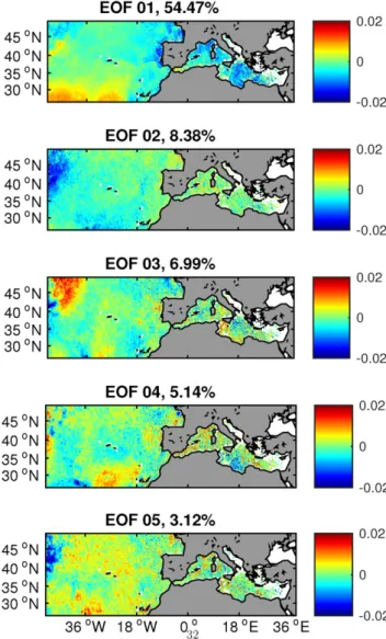
The DINEOF reconstruction used in this work consists of 5 EOF modes that explain 78% of the initial variance (Table 2). Thefive spatial EOFs are shown inFig. 12and the temporal ones inFig. 13. These show the spatial and temporal evolution of the Gulf Stream and its meanders,

Fig. 8. Two TSG transects at their original temporal resolution (~ 5 min) in the North Atlantic Ocean and their SMOS and DINEOF interpolated to the TSG positions. Transect a (top panel) gets closer to the coast and this is reflected in the larger fresh bias in the DINEOF data.

Fig. 9. Example of initial (top panel) and reconstructed DINEOF SSS data (bottom panel) for 21 July 2013.

Fig. 10. Time series of SSS at the Douro (top panel) and the Gironde (bottom panel) river plumes. The boxes delimiting these two zones are shown inFig. 9.

Fig. 11. Example of the signal of the Douro river plume in SSS (left panel) and chlorophyll-a concentrchlorophyll-ation (right pchlorophyll-anel) chlorophyll-averchlorophyll-aged over the period 26 Februchlorophyll-ary to 5 Mchlorophyll-arch 2013.

and the subtropical SSS maximum. Other features that appear to have a signal in the EOF basis are the Alboran Sea (EOF 1) that becomes saltier through the year, and the plumes of the Gironde (EOF 1) and Douro riv-ers (EOFs 1 and 3). An in-depth study of the signature of these three fea-tures in the SMOS SSS needs to be carried on in future works.

Two of the EOFs rejected by DINEOF (i.e. not used in the_final recon-struction) present a pattern that is easily attributed to the errors at the edges of the satellite swath (Fig. 14). These patterns, with a periodicity of 18 days, represent about 2.8% of the initial variance and have been isolated by the EOF decomposition. Because these EOF modes are not retained in the EOF basis used for the DINEOF reconstruction, the errors at the edges of the swath are effectively removed from the dataset. This approach allows retaining more information in the initial dataset while removing constant errors. The length of the temporal covariancefilter has an effect in the detection of these patterns: when using afilter of a length of 18 days, these features were not captured in any EOF mode (results not shown), indicating that the signal was being averaged with-in the data. By selectwith-ing a shorterfilter length we were able to smooth the data in time but at the same time to isolate and remove these fea-tures from the data, which validates the choice of a 14-dayfilter length. 5. Conclusions

A procedure to obtain SMOS SSS data at a daily time step and with a spatial resolution of 0.15° × 0.15° using DINEOF has been presented. It

has been shown that DINEOF allows retrieving complete daily_{fields of} SSS with reduced noise, by detecting and removing outliers in the initial fields. A sensitivity study has been carried out to determine the optimal configuration of DINEOF, namely the length of a temporal covariance fil-ter (aiming at improving the temporal coherence of the dataset) and the outlier detection threshold. The truncated EOF basis used to compute thefinal SSS data is able to reject noise, as well as errors present at the edges of the satellite swath. Comparison with in situ data shows that in addition to the increased coverage, the correlation is improved and the centered RMS error is reduced. The centered RMS error between the DINEOF SSS estimates (at the highest spatial and temporal resolu-tion) and TSG data in open waters is as low as 0.2. When considering the whole domain of study (including the Mediterranean Sea) the cen-tered RMS increases to 0.55. Constant biases present in the initial dataset cannot be corrected using DINEOF, as these persistent signals are probably in the most dominant EOFs, and therefore affect thefinal dataset as well. The bias has been shown to be of−0.3 in open waters (in comparisons with TSG data) and−0.57 over the whole domain of study.

The presence of several features in the reconstructed dataset has been assessed: the Gulf Stream and the subtropical salinity maximum at the large spatial scale, and the fresh plumes of the Gironde and Douro rivers at the small scale. The presence of the river plumes in the SMOS data is evidenced by a localized salinity minimum that is superimposed to constant biases present along the coast and that are due to the presence of land masses. Because of these biases, the study of these plumes cannot be done quantitatively, but the DINEOF SSS data allow assessing their spatial extent and variation with time. The time series of SSS at the vicinity of the Gironde estuary correlates well to the river discharge, with the minimum SSS occurring during aflood event in June 2013. Regarding the Douro river plume, it has been shown that it presents a shape and size similar to what is observed in chlorophyll-a concentration data. A careful validation of these results as well as an assessment of the spatial and temporal scales of these river plumes must be carried out using other sources of data (satellite and in situ) and hydrodynamic models.

While errors still remain in the DINEOF reconstruction, these can be further reduced through bias correction procedures and through spatial and temporal averaging of the data, as for example the one proposed by

Kolodziejczyk et al. (2016-in this issue). The aim of this work was to provide SSS data at the highest resolution possible in space and time in order to remove errors at their source. Future work includes the mul-tivariate analysis of SSS with variables like temperature and precipita-tion, in order to establish the correlation between them and use this information in the improvement of the SSS estimations. The assessment of the spatial and temporal variability of the river plumes observed in this work, and their correlation with river discharge and turbidity will be also the focus of future studies.

Fig. 12. Five EOF spatial modes retained for the DINEOF reconstruction. The percentage in each title provides the explained variance.

Acknowledgments

This work has been carried out within the project“Improving Sea Surface Salinity Estimates through Multivariate and Multisensor Analy-ses” (http://www.gher.ulg.ac.be/WP/), funded by the European Space Agency (4000110775/14/I-BG) “Support to Science (STSE) PATH-FINDERS” call.

In situ data providers, Coriolis Data Centre (http://www.coriolis.eu. org) and World Ocean Database (http://www.nodc.noaa.gov/) are also acknowledged. Sea surface salinity data derived from thermosalinograph instruments installed onboard voluntary observing ships were collect-ed, validatcollect-ed, archivcollect-ed, and made freely available by the French Sea Surface Salinity Observation Service (http://www.legos.obs-mip.fr/ observations/sss/). Chlorophyll-a concentration data were obtained throughhttp://oceancolor.gsfc.nasa.gov/. We also thank Manuel Arias for his feedback on the use of SMOS salinity qualityflags.

References

Alvera-Azcárate, A., Barth, A., Beckers, J. -M., & Weisberg, R. H. (2007). Multivariate recon-struction of missing data in sea surface temperature, chlorophyll and wind satellite fields. Journal of Geophysical Research, 112, C03008.http://dx.doi.org/10.1029/ 2006JC003660.

Alvera-Azcárate, A., Barth, A., Rixen, M., & Beckers, J. -M. (2005). Reconstruction of incom-plete oceanographic data sets using Empirical Orthogonal Functions. Application to the Adriatic Sea surface temperature. Ocean Modelling, 9, 325–346.http://dx.doi. org/10.1016/j.ocemod.2004.08.001.

Alvera-Azcárate, A., Barth, A., Sirjacobs, D., & Beckers, J. -M. (2009).EOF expansions for the reconstruction of missing data using DINEOF. Ocean Science, 5, 475–485. Alvera-Azcárate, A., Sirjacobs, D., Barth, A., & Beckers, J. -M. (2012).Outlier detection in

satellite data using spatial coherence. Remote Sensing of Environment, 119, 84–91. Alvera-Azcárate, A., Vanhellemont, Q., Ruddick, K., Barth, A., & Beckers, J. -M. (2015).

Anal-ysis of high frequency geostationary ocean colour data using DINEOF. Estuarine, Coastal and Shelf Science, 159, 28–36.

Barth, A., Beckers, J. -M., Troupin, C., Alvera-Azcárate, A., & Vandenbulcke, L. (2014). divand-1.0: n-dimensional variational data analysis for ocean observations. Geoscientific Model Development. 7. (pp. 225–241), 225–241 (URLhttp://www.geosci-model-dev. net/7/225/2014/).

Beckers, J. -M., & Rixen, M. (2003).EOF calculations and datafilling from incomplete oceanographic data sets. Journal of Atmospheric and Oceanic Technology, 20(12), 1839–1856.

Boutin, J., Martin, N., Reverdin, G., Morisset, S., Yin, X., Centurioni, L., & Reul, N. (2014).Sea surface salinity under rain cells: SMOS satellite and in situ drifters observations. Journal of Geophysical Research, Oceans, 119, 5533–5545.

Boutin, J., Martin, N., Xiaobin, Y., Font, J., Reul, N., & Spurgeon, P. (2012).First assessment of SMOS data over open ocean: Part II— Sea surface salinity. IEEE Transactions on Geoscience and Remote Sensing, 50(5–1), 1662–1675 (50 (5), 1662–1675).

Boyer, T., Antonov, J. I., Baranova, O. K., Coleman, C., Garcia, H. E., Grodsky, A., ... Zweng, M. M. (2013). World Ocean Database 2013, NOAA Atlas NESDIS 72. In S. levitus (Ed.), a. mishonov, technical ed. Edition. MD: Silver Spring (209 pp.,http://doi.org/10.7289/ V5NZ85MT).

Brasseur, P., Beckers, J. M., Brankart, J. M., & Schoenauen, R. (1996).Seasonal temperature and salinityfields in the Mediterranean Sea: Climatological analyses of a historical data set. Deep-Sea Research Part I, 43, 159–192.

Fournier, S., Chapron, B., Salisbury, J., Vandemark, D., & Reul, N. (2015).Comparison of spaceborne measurements of sea surface salinity and colored detrital matter in the amazon plume. Journal of Geophysical Research, Oceans, 120, 3177–3192.

Grodsky, S., Reverdin, G., Carton, J., & Coles, V. (2014).Year-to-year salinity changes in the Amazon plume: contrasting 2011 and 2012 Aquarius/SACD and SMOS satellite data. Remote Sensing of Environment, 140, 14–22.

Iglesias, I., Couvelard, X., Avilez-Valente, P., & Caldeira, R. (2016).Numerical study of the Douro River plume: Mediating the inner- and cross-shelf dynamics. Ocean Dynamics (submitted for publication).

Jalón-Rojas, I., Schmidt, S., & Sottolichio, A. (2015).Turbidity in thefluvial gironde estuary (southwest france) based on 10-year continuous monitoring: Sensitivity to hydrolog-ical conditions. Hydrology and Earth System Sciences, 19, 2805–2819.

Kolodziejczyk, N., Boutin, J., Vergely, J. -L., Marchand, S., Martin, N., & Reverdin, G. (2016). Mitigation of systematic errors in smos sea surface salinity. Remote Sensing of Environment, 180, 164–177 (in this issue).

Kolodziejczyk, N., Hernandez, O., Boutin, J., & Reverdin, G. (2015).SMOS salinity in the subtropical North Atlantic salinity maximum: 2. Two-dimensional horizontal ther-mohaline variability. Journal of Geophysical Research. Oceans, 120, 972–987. Lagerloef, G., & Font, J. (2010).SMOS and aquarius/SAC-D missions: The era of spaceborne

salinity measurements is about to begin. Springer (Ch. 3).

Lagerloef, G., Schmitt, R., Schanze, J., & Kao, H. -Y. (2010).The ocean and the global water cycle. Oceanography, 23(4), 82–93.

Mendes, R., Vaz, N., Fernndez-Nvoa, D., da Silva, J., deCastro, M., Gmez-Gesteira, M., & Dias, J. (2014).Observation of a turbid plume using MODIS imagery: The case of Douro es-tuary (Portugal). Remote Sensing of Environment, 154, 127–138.

Reul, N., Chapron, B., Lee, T., Donlon, C., Boutin, J., & Alory, G. (2014).Sea surface salinity structure of the meandering Gulf Stream revealed by SMOS sensor. Geophysical Research Letters, 41, 3141–3148.

Sirjacobs, D., Alvera-Azcárate, A., Barth, A., Lacroix, G., Park, Y., Nechad, B., ... Beckers., J. -M. (2011).Cloudfilling of ocean color and sea surface temperature remote sensing products over the Southern North Sea by the Data Interpolating Empirical Orthogonal Functions methodology. Journal of Sea Research, 65(1), 114–130.

Troupin, C., Barth, A., Sirjacobs, D., Ouberdous, M., Brankart, J. -M., Brasseur, P., ... Beckers, J. -M. (2012). Generation of analysis and consistent errorfields using the data inter-polating variational analysis (diva). Ocean Modelling (URLhttp://hdl.handle.net/ 2268/125731).

Yin, X., Boutin, J., Martin, N., & Spurgeon, P. (2012).Optimization of L-band sea surface emissivity models deduced from SMOS data. IEEE Transactions on Geoscience and Remote Sensing, 50(5), 1414–1426.

Yin, X., Boutin, J., Martin, N., Spurgeon, P., Vergely, J. -L., & Gaillard, F. (2014).Errors in SMOS Sea surface salinity and their dependency on a priori wind speed. Remote Sensing of Environment, 146, 159–171.

Zine, S., Boutin, J., Font, J., Reul, N., Waldteufel, P., Gabarró, C., ... Delwart, S. (2008). over-view of the smos sea surface salinity prototype processor. IEEE Transactions on Geoscience and Remote Sensing, 46(3), 621–645.

Fig. 14. EOF modes 6 and 7, not retained in the DINEOF reconstruction. These modes represent error at the edges of the swath, which are reinforced at the 18-day repeat cycle of SMOS and therefore isolated as two distinct EOF modes. Note that the temporal EOFs have a quarter-phase lag between them.