1 INTRODUCTION
In many cases, special devices such as viscous dampers must be added to structures, in order to compensate for their bad dynamic behaviour.
Viscous dampers are nowadays commonly used in wind and seismic engineering. Some of them can sometimes be assumed to exhibit a linear behaviour, whereas other damping devices are characterised by a non linear behaviour, most of the time described by a power law (F = C.Vα - α<1). Compared to lin-ear dampers, such devices present the advantage to dissipate a significantly greater amount of energy for identical maximum forces and displacements. How-ever they are obviously more complicated to manage in the context of numerical simulations.
2 NON LINEAR DAMPERS
The most basic test that can be realized to deter-mine the behavior of a dash-pot consists in forcing the ends of the device to move with a harmonic rela-tive displacement. A first characterization can then be obtained by varying the frequency of the periodic imposed displacement.
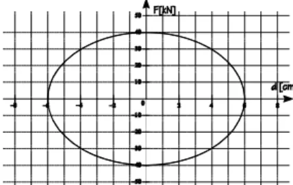
After stabilization of the response, the dash-pot describes a characteristic curve in a Force-Displacement (FD) diagram. For example, for a per-fectly linear dash-pot, the force is proportional to the relative velocity : ) ( ) (t Cv t F = (1)
Hence, a harmonic imposed displacement would give : ) sin( ) (t A t d = ω (2) ) cos( ) ( ) cos( ) (t A t F t CA t v = ω ω ⇒ = ω ω (3)
Removing the time parameter between Equations 2 and 3 provides the equation of the curve in the FD diagram : 1 2 2 = + ω CA F A d (4) This well-known elliptic equation characterizing
a linear dash-pot is plotted on figure 1.
Figure 1. Characteristic curve of a linear damper in the Force-Displacement diagram
Let us consider now a non linear damper characterized by the power law :
[ ]
α ) ( ) (t C v t F = (5)Analysis of Linear Structures With Non Linear Dampers
V.Denoël
Department of Mechanics of materials and Structures, University of Liège, Belgium
H.Degée
Department of Mechanics of materials and Structures, University of Liège, Belgium
ABSTRACT: This paper provides information about the numerical simulation of the dynamic behaviour of linear structures including non linear dampers, for which the relation between the damping force and the ve-locity is described by a power law. A first part of the paper deals with single degree of freedom (SDOF) sys-tems, with a particular emphasis on the resolution of the non linear equation allowing to compute the damping force corresponding to a given velocity. A second part deals with multi degree of freedom (MDOF) systems, and presents a special algorithm to study the behaviour of structures with a very small number of non linear components.
The equation of the characteristic curve in the FD diagram is then given by :
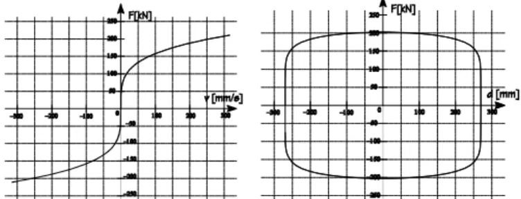
1 2 / 1 / 1 2 = + ω α α A C F A d (6) As an illustration, Figure 2 represents the
constitu-tive law and the FD curve of a non linear damper.
Figure 2. Representation of a power constitutive law ( α = 0.25 ; C = 50 kN / (mm/s)0.25 and the corresponding FD curve.
In equation (6), the linear behavior can be ob-tained by setting α = 1. When the parameter α ap-proaches 0, the behavior becomes “rigid perfectly viscous” and the shape of the FD curve tends to-wards a rectangle.
Here comes the first advantage of non linear dampers : as the area enclosed inside the FD curve represents the amount of energy dissipated per cycle, a non linear damper can dissipate a larger amount of energy than a linear one for identical maximum force and displacement.
The maximum benefit corresponding to a “rigid perfectly viscous” damper can be easily computed by comparing the area of an ellipse with the area of the rectangle circumscribing this ellipse :
% 3 , 27 4 = − = ππ Q (7)
Another reason for which non linear dampers are used is not based on energy considerations but rather on a security design. As this kind of device is gener-ally designed to improve the behavior of a structure under probabilistic actions (earthquake, wind,…), the maximum level of the solicitation cannot be de-termined exactly.
As a consequence, the maximum velocity of any point of the structure cannot be determined either. The maximum force applied by a linear damper is then unknown whereas the maximum force applied by a non linear damper can be limited as much as wanted by choosing a sufficiently low value for pa-rameter α. So, in case of unexpected increase of the external forces, a non linear damper won’t apply in-tolerable forces on the structure.
3 ANALYSIS OF SDOF SYSTEMS
The equation of motion corresponding to a single degree of freedom system with constant mass and stiffness and with power law damping is represented by this non linear second order differential equation:
[ ]
( ) ( ) ( ) )(t c u t k u t p t u
m && + & α + = (8)
The two main characters of this equation (differ-ential and non linear) are generally considered the one after each other.
3.1 The differential character
The large number of methods allowing to solve the well-known linear equation is of course beyond the scope of this paper.
This paragraph presents however a short sum-mary of the resolution methods in the time domain.
Basically, this first method considers the external force as a succession of short impulses. For each of these, the response can be computed and the total re-sponse at time t is then obtained as a sum of all the contributions associated to the effects of each im-pulse.
Analytically, the duration of each impulse tends towards zero and the sum becomes an integral. The method explained here above leads to the well known Duhamel integral :
( )
∫
− = t d d d e p m t u 0 . sin ) ( 1 ) ( τ ω τ τ ω ξωτ (9)whereξ is the damping coefficient and ωd is the damped pulsation of the system.
Regarding the kind of problem that has to be treated here, this method has the great disadvantage of being based on the superposition principle, which is only valid for linear structures.
Numerically, it is possible to develop methods which are not based on the superposition principle. The so-called “step by step” methods are not based on a superposition of different contributions any-more, but rather on a discretization of time in small time steps. Assumptions are then made regarding displacement, velocity and acceleration at the end of each time step. Together with the discretized equa-tion of moequa-tion, it is then possible to compute the re-sponse at the end of the time step. A huge number of techniques have been developed amongst which the most famous are : constant or linear acceleration method, central difference method, Newmark method, Houbolt’s method, Wilson-θ method, HHT method.
Since the purpose of the paper deals with solving a non linear equation, a step by step method has been chosen. The developments are made with New-mark method.
Classical linear Newmark method can be adapted for solving the non linear Equation 8. The displace-ment at the end of a time step is then given by :
− + ∆ + ∆ + = + ∆ t+∆t t+∆t t ut ut t u t m p u k t m && & 4 4 . 4 2 2 C
[ ]
u&t+∆t α (10) where the subscripts t and t + ∆t denote respectivelythe response at the beginning and at the end of the time step.
As the velocity at the end of the time step can be expressed in terms of the displacement at the end of the step, Equation 10 can be rewritten in the form :
[ ]
+ ∆ + ∆ + = +∆ ∆ + t t t t t t t u u t u t m p u F 42 4 & && (11) The second part of the equation is a known quantityand the function F is defined by :
[ ]
[
(
)
]
α t t t t t t t t k u C u u t m u F +∆ +∆ + +∆ +∆ + ∆ = 4 2 & (12)3.2 The non linear character
The first considerations related to the differential character of the equation allow to transform the original problem to the resolution of a series of equations like Equation 11. This latter is the non lin-ear equation that has to be solved. The next para-graphs illustrate different methods to solve it. For convenience, Equation 11 will be rewrited :
[ ]
x fF = (13)
where x represents the unknown ut+∆t. 3.2.1 The Newton-Raphson method
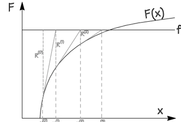
The most famous method for solving such prob-lems is the Newton-Raphson (NR) method summa-rized in figure 3.
Starting from an approximation x(0) of the solu-tion, the method consists in considering the intersec-tion x(1) of the tangent to the function F(x) at point x(0) with the horizontal F(x) = f as a better approxi-mation of the solution. Mathematically, this can be expressed by : ) ( ’ ) ( ) ( ) ( ) ( ) 1 ( i i i i x F x R x x + = + (14)
At each iteration the remainder, difference be-tween the target value f and the function F(x(i)), should decrease until a convergence criterion is veri-fied : precision i f R − ≤10 ) ( (15)
Figure 3 : Illustration of the Newton-Raphson method for solv-ing non linear equations
This method encounters several problems with Equation 11 which has to be solved. They result mainly from the vertical slope inflexion point in the function F. Indeed, the first term in this function (see Eq. 12) is linear whereas the second one has the same shape as the constitutive law. The function F exhibits therefore a vertical slope inflexion point.
Despite its very fast convergence (2nd order), the NR method misbehaves in the vicinity of inflexion points. This is illustrated in figure 4.
Figure 4 : Convergence problems of the Newton-Raphson method around inflexion points
The original method is then in general replaced by the modified-NR method which, in case of non convergence, continues the iterations with a fixed slope larger than the slope at the inflexion point; this enables then to reach the convergence.
3.2.2 The Regula Falsi method
As in the equation to solve, the slope at the inflexion point is vertical, it is impossible to find a larger slope and to proceed to the modified-NR method. It is then necessary to use another method.
Only first order methods can succeed in crossing inflexion points. To this scope, the regula falsi method can be used.
The basic idea is to turn around a reference point at each iteration and, during the iterative procedure, to modify the position of this point in order to opti-mise the convergence. The method works always
with the reference point and with a moving point ob-tained by the intersection of the horizontal F = f with the line going through the reference point and the previous point. Mathematically, it is expressed by :
) ( ) ( ) ( ) ( () ) ( ) ( ) ( ) 1 ( f i i i f i i x R x R x R x x x x − − + = + (16)
Figure 5 shows an example where the reference point xf is not modified, whereas Figure 6 shows
an-other one where the reference point xf is modified at
each iteration. The condition for changing the refer-ence point is simple : if the new remainder has the same sign as the remainder at the reference point, then it should be changed to the previous point, else it must be kept unchanged.
Figure 5 : Regula Falsi method. The reference point is un-changed from beginning till end of the iterations
Figure 6 : Regula Falsi method. The reference point is changed at each iteration.
The regula falsi method is also an iterative method and the convergence criterion used to stop can be expressed by Equation 15 as for the NR method.
3.2.3 Conclusion
The regula falsi is a method which will always lead to convergence but slowlier than the NR method. So, combining these two methods, the best is to use NR where the convergence can be reached by this method and to use the regula falsi elsewhere.
In practice, this can be achieved by always begin-ning with the NR method; once the solutions are go-ing back and forth a limit value, we switch to the regula falsi method.
3.3 Example
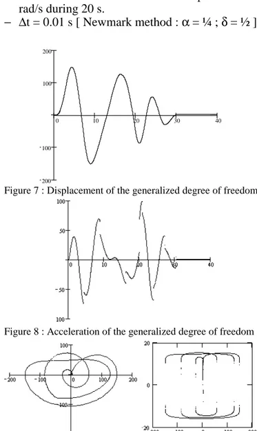
Here is the response of a single degree of freedom characterized by the following parameters :
− Mass : m = 1 − Stiffness : k = 1
− Damping : C = 10 ; α = 0.1
− External Force : Harmonic with a pulse ω = 0,5 rad/s during 20 s. − ∆t = 0.01 s [ Newmark method : α = ¼ ; δ = ½ ] 0 10 20 30 40 200 100 100 200
Figure 7 : Displacement of the generalized degree of freedom
Figure 8 : Acceleration of the generalized degree of freedom
Figure 9 : Phase diagram and FD diagram of the dash-pot
3.4 Observations
− In Figure 7, the free displacement looks ‘classic’ between 20 s and 30 s. After this, the oscillator seems to be frozen but this is of course not a re-sidual displacement. The system doesn’t have enough energy anymore to go beyond the elbow of the constitutive law of the dash-pot. For the rest of the computation the viscosity is then very high and it takes a very long time to reach a zero displacement.
− In Figure 8, the acceleration seems to be discon-tinuous. In fact, this is the result of passing trough the elbow : the acceleration is of course perfectly continuous but varying very fast. Further investi-gation, using a non constant time step, allows to
compute more precisely the points in the fast varying zone.
− In Figure 9, it is possible to recognize the classi-cal rectangular shape of a non linear dash-pot in the FD diagram. Several curves are covered, be-cause the response is not harmonic. Furthermore, because of the constant time step, the response in the fast varying zone is less precise than for higher velocities.
− With a precision factor (See Eq. 15) of 8, the mean number of iterations was 3 iterations per time step for which the NR method converged and 15 to 20 iterations otherwise (in these are in-cluded the NR iterations which did not converge).
4 ANALYSIS OF MDOF SYSTEMS
Basic developments concerning the differential and non linear characters of Equation 8 can be adapted in order to solve a multi-degree of freedom system.
Obviously, the main difference lies in the great number of degrees of freedom, implying a large sys-tem to solve. For complex structures, the size of the system can often reach 104 or 105 DOF.
Amongst these degrees of freedom, only a small part is concerned with the non linear dampers. The rest of the structure can generally be considered to behave linearly. This could be for example the case in the design of damping devices for a structure en-countering troubles due to wind.
4.1 The equation of motion
Similarly to the SDOF system, a step-by-step method is first used to transform the non linear dif-ferential system to several systems of non linear equations. With the Newmark method, this system can be written in the following form (to compare to Equation 11) :
[ ]
A{ }
u t+∆t +{
FCD,nonlin(
{
u&t+∆t(
{ }
ut+∆t)
}
)
}
={ }
b t (17) where[ ]
[ ] [ ]
M K t A + ∆= 42 (
[ ]
M and[ ]
K are the mass and stiffness matrices of the structure) and{ } { }
[ ]
{ }
{ } { }
+ + ∆ + ∆ + = t+∆t t t t t u u t u t M P b . 42 4 & &&(
[ ]
[
]
)
{ } { }
+ ∆ + Dlin t t S u u t C C , . 2 & (18)in which [C ] and [S CD,lin] represent respectively the structural Rayleigh damping matrix and the concen-trated linear damping matrix (linear dash-pots).
Equation 16 represents the non linear system of equations to be solved with the NR method. The or-der of this system is the total number of degrees of freedom in the structure. Written like this, the addi-tional iterations required by the non linearity’s imply to iterate on the full system. To avoid this, it is inter-esting to reduce the number of equations to handle in the NR iterations through a static condensation. 4.2 Static condensation
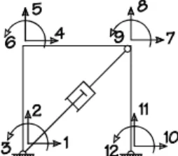
Let us qualify by the term ‘non linear’ a degree of freedom which is directly related to a non linear damper (i.e. a translation of a node at which a non linear dash-pot is attached). For example, in figure 10, the non linear degrees of freedom are the DOF 1,2,7 and 8.
Figure 10 . Illustration of the definition of the non linear DOF
We can now sort the equations in the system (Eq. 17) by placing the non linear DOF above the others :
[ ] [ ]
[ ] [ ]
{ }
{ }
(
{ }
)
{ }
{ }
L t N t t N nonlin CD t t L N LL LN NL NN b b u F u u A A A A = + +∆ ∆ + 0 , (19) The subscripts ‘L’ and ‘N’ are used respectively for linear and non linear DOF. In Equation 19, only the group of equations corresponding to the first line is non linear. The other equations remain linear since the non linear term is zero (the damper do not apply any direct force on these nodes).The second line of this 2 x 2 system gives :
{ }
uL[ ]
ALL(
{ }
bL[ ]
ALN .{ }
uN)
1 −
= −
(20) After substitution of Equation 20 in Equation 19, we
obtain a new reduced system:
[ ]
A{ }
u{
F}
{ }
f t t nonlin CD N + , +∆ = . * (21) where[ ] [ ] [ ][ ] [ ]
A* ANN ANL .ALL .ALN 1 − − = and{ } { }
f bN[ ][ ]
ANL .ALL .{ }
bL 1 − − = .The order of the new system (Eq. 21) is thus reduced to its minimum value i.e. the number of non linear degrees of freedom. The NR (or regula falsi) method can then be applied to compute the response of the non linear degrees of freedom at the end of the time step.
Then, equation 20 can be used to compute the re-sponse of the linear degrees of freedom. This huge
amount of values are computed only after conver-gence and not at each iteration of the NR method !
Going further into the developments is of course beyond the scope of this paper. Interested readers can found the full developments and discussions about this method in Reference 1.
4.3 Example
The example consists in determining the response of a 37 meter high bridge pier modelled by 11 beam elements (A=14.3 m² ; I=38.3 m4 ; E = 23600 MPa) This pier is subjected to a very particular ground motion shaking characterized by this acceleration :
t t ug ∆ = . 8 sin && (22)
Two different dampers are placed at the head of the pier in order to reduce the effects of the ground motion :
− A first one with a bilinear constitutive law (C1 =
4.5E8 N.s/m ; C2=4E6 N.s/m ; vlim = 8E-4 m/s )
− A second one with the classic power law (C = 1E6 N.(s/m)0.2 ; α = 0.2 )
In order to investigate the possibility of replacing a power law damper by a bilinear law damper, the two dash-pots have been chosen in such a way that their behavior is the most similar.
-0,002 -0,0015 -0,001 -0,0005 0 0,0005 0,001 0,0015 0,002 0 0,5 1 1,5 2 2,5 3 3,5 4 Time [s] D isp lace m en t [ m ]
Bilinear law Power law
Figure 11 : Displacement at the head of the pier (for both dampers) -600 -400 -200 0 200 400 600 -0,002 -0,0015 -0,001 -0,0005 0 0,0005 0,001 0,0015 0,002 Displacement [m] Fo rc e [ k N ]
Bilinear law Power law
Figure 12 : FD diagrams of the dash-pots.
Figure 11 represents the displacement at the head of the pier (for both dampers), whereas Figure 13 represents their FD curve.
4.4 Observations
− The FD diagram has the classical shape, excepted in the corners where inertial effects (participation of the second vibration mode) modify slightly the shape which would be obtained with a SDOF sys-tem ;
− Results related to the power law damper can be approached quite precisely with a bilinear damper which is consuming 2.8 times less iterations than the power law dash-pot. Advantage could then be taken of the bilinear law, provided a good equiva-lence is ensured.
5 CONCLUSIONS
This document first presented solutions to the nu-merical problems encountered during the analysis of structures including power law dampers, problems related to the vertical inflexion point in the constitu-tive law.
In a second step, by considering SDOF systems, the paper points out the characteristics of the re-sponse of structures constituted of non linear damp-ers (residual displacement; pseudo-discontinuous acceleration).
Furthermore, through the analysis of MDOF sys-tems, it introduces and justifies the use of the static condensation method for linear structures with con-centrated non linearity’s. This method reduces the size of the system to its minimum, which enables a huge decrease of the computation time.
Finally, through an example, the paper shows that, provided good equivalence is chosen, a power law dash-pot can be efficiently replaced by a bilinear law dash-pot. In this case the numerical approach is much easier since the vertical inflexion point disap-pears.
6 REFERENCES
1 V. Denoël. Calcul sismique des ouvrages d’art, Gra-duation project, University of Liège, (2001).
2 R.W. Clough and J. Penzien, Dynamics of the
struc-tures, Mc Graw-Hill, London, Second Edition, (1993).
3 J.M. Ortega and W.C. Rheinbold, Iterative solution of
non-linear equations in several variables, Academic
![Figure 11 : Displacement at the head of the pier (for both dampers) -600-400-2000 200400600-0,002-0,0015-0,001-0,0005 0 0,0005 0,001 0,0015 0,002 Displacement [m]Force [kN]](https://thumb-eu.123doks.com/thumbv2/123doknet/5643570.136508/6.892.52.436.627.843/figure-displacement-head-pier-dampers-displacement-force-kn.webp)
