Zigzag antiferromagnetic quantum ground state in monoclinic honeycomb lattice antimonates A3Ni2SbO6 (A=Li, Na)

A zigzag antiferromagnetic quantum ground state in monoclinic

honeycomb lattice antimonates A3Ni2SbO6 (A=Li, Na)

E.A. Zvereva1,*, M.I. Stratan1, Y.A. Ovchenkov1, V.B. Nalbandyan2, J.-Y. Lin3, E.L. Vavilova4, M.F.Iakovleva4, M. Abdel-Hafiez,5,6,7 A.V. Silhanek,5X.-J. Chen7, A. Stroppa,8

S. Picozzi,8 H. O. Jeschke,9 R. Valentí,9 and A.N. Vasiliev1,10,11 1_{Faculty of Physics, Moscow State University, 119991 Moscow, Russia}

*_{zvereva@mig.phys.msu.ru}

2_{Chemistry Faculty, Southern Federal University, 344090 Rostov-on-Don, Russia} 3_{National Chiao Tung University, Hsinchu, Taiwan, 300 R.O.C.}

4_{Zavoisky Physical-Technical Institute (ZPhTI) of the Kazan Scientific Center of the Russian} Academy of Sciences, 420029 Kazan, Russia

5_{Département de Physique, Liége University-Belgium, B-4000 Liege, Belgium} 6_{Faculty of science, Physics department, Fayoum University, 63514 Fayoum, Egypt} 7_{Center for High Pressure Science and Technology Advanced Research, 1690 Cailun Rd.,}

Shanghai, 201203, China 8_{CNR-SPIN, L'Aquila, Italy}

9_{Institut für Theoretische Physik, Goethe-Universität Frankfurt, Max-von-Laue-Straße 1, 60438} Frankfurt am Main

10_{Theoretical Physics and Applied Mathematics Department, Ural Federal University,} 620002 Ekaterinburg, Russia

11_{National University of Science and Technology "MISiS", Moscow 119049, Russia}

Abstract

We present a comprehensive experimental and theoretical study of the electronic and magnetic properties of two quasi-two-dimensional (2D) honeycomb-lattice monoclinic compounds A3Ni2SbO6 (A=Li, Na). Magnetic susceptibility and specific heat data are consistent with the onset of antiferromagnetic (AFM) long range order at low temperatures with Néel temperatures ~ 14 and 16 K for Li3Ni2SbO6 and Na3Ni2SbO6, respectively. The effective magnetic moments of 4.3 B/f.u. (Li3Ni2SbO6) and 4.4 B/f.u. (Na3Ni2SbO6) indicate that Ni2+ is in a high-spin configuration (S=1). The temperature dependence of the inverse magnetic susceptibility follows the Curie-Weiss law in the high-temperature region and shows positive values of the Weiss temperature ~ 8 K (Li3Ni2SbO6) and ~12 K (Na3Ni2SbO6) pointing to the presence of non-negligible ferromagnetic interactions, although the system orders AFM at low temperatures. In addition, the magnetization curves reveal a field-induced (spin-flop type) transition below TN that can be related to the magnetocrystalline anisotropy in these systems. These observations are in agreement with density functional theory calculations, which show that both antiferromagnetic and ferromagnetic intralayer spin exchange couplings between Ni2+ ions are present in the honeycomb planes supporting a zigzag antiferromagnetic ground state. Based on our experimental measurements and theoretical calculations we propose magnetic phase diagrams for the two compounds.

75.30.Kz; 75.10.Dg; 75.30.Gw; 75.30.Et

I. Introduction

Layered oxides of alkali and transition metals are presently being intensively investigated due to their potential applications as solid electrolytes and electrode materials in modern ionics [1,2], as thermoelectric materials [3,4] and even as superconductors [5,6]. Recently, a lot of

attention has been focused on a new generation of layered complex metal oxides with honeycomb-based crystal structure [7-36] with phases such as A+3M2+2X5+O6 and A+2M2+2Te6+O6 (A=Li, Na; X=Bi, Sb; M is transition metal) where ordered mixed-layers of magnetic cations M2+ and X5+ (or M2+ and Te6+) alternate with non-magnetic alkali metal layers. The crystal structures are very soft and even slight modification, for example in a stacking mode of alternating layers, results in drastic changes in the magnetic properties. In turn, increasing the distance between magnetically active layers leads to a weakening of interplanar spin interactions and concomitant possible lowering of the magnetic dimensionality of the systems.

The honeycomb arrangement of cations within the magnetically active layers provides a large variety of quantum ground states. The classical (S=infinity) Heisenberg model on a honeycomb lattice with nearest-neighbor antiferromagnetic exchange coupling J1 is known to have a Néel ordered ground state (Fig. 1) [37]. Adding frustrating second and third neighbor interactions J2 and J3 as well as quantum corrections leads to a complex phase diagram. Depending on the spin value and signs and ratios J2/J1 and J3/J1, different types of spin ordering on the honeycomb lattice can be realized including Néel, zigzag, stripy, and different spiral orders (Fig. 1) [38]. Moreover, it has been experimentally reported that a non-magnetic ground state can also be achieved on honeycomb lattices in the presence of either lattice distortion or frustration [10-15,30,35]. For example, a spin-gap behavior was found for O3-derived Cu2+ honeycomb compounds Na2Cu2TeO6 [10,11], Na3Cu2SbO6 [11-15,35] and related delafossite-derived honeycomb S=1/2 compound Cu5SbO6 (Cu+3Cu2+2Sb5+O6) [30]. Antiferromagnetic

zigzag ordering in the honeycomb plane was observed recently for the structurally related

honeycomb-lattice delafossites Cu3Ni2SbO6 and Cu3Co2SbO6 [31]. No long-range magnetic order was found for honeycomb Na3LiFeSbO6 and Na4FeSbO6 and Li4MnSbO6 probably due to disorder and frustration effects [34,36]. At the same time, honeycomb-ordered O3-derived phases Na3M2SbO6 (M=Cu, Ni, Co) [17,19,31], Li3Ni2SbO6 [20], Li3Ni2BiO6 [21], Na3Ni2BiO6 [33], as well as P2-derived Na2M2TeO6 (M=Co, Ni) [18,19], were found to order antiferromagnetically at low temperatures but their real quantum ground state remains unknown and requires joint experimental and theoretical efforts to be determined. The influence of the interlayer coupling and of the anisotropy on the ground state in such systems is largely unexplored at present.

FIG. 1. 2D honeycomb-lattice Heisenberg model with up to third neighbor exchanges, J1,2,3, and spin-configuration diagrams for Neel, zigzag, stripy and FM order.

The present work is devoted to the investigation of new quasi two-dimensional (2D) honeycomb-lattice compounds Li3Ni2SbO6 and Na3Ni2SbO6. We combine magnetic susceptibility, magnetization, specific heat, electron spin resonance and nuclear magnetic resonance measurements with density functional theory calculations and uniquely identify the appropriate magnetic model for these systems as well as the corresponding applied field-temperature phase diagram.

Basic magnetic properties of Li3Ni2SbO6 and Na3Ni2SbO6 have been reported recently [17,20,22], but a systematic analysis of their electronic and magnetic behavior is missing. Ordered structure of Li3Ni2SbO6 was refined in the space group C2/m [20]. For Na3Ni2SbO6, the initial structure determination was complicated by multiple stacking faults. Nevertheless, it was unambiguously shown that the general layout of the structure is the same as in Li3Ni2SbO6 [22, 17]. Therefore, our analysis of magnetic interactions was based on a C2/m model constructed on

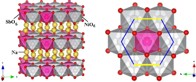
lattice parameters and ionic radii sums. Quite recently, it was reported about preparation of both ordered and disordered forms of Na3Ni2SbO6 [39]. It was confirmed that complete Ni/Sb ordering within each layer exists even in “disordered” apparently rhombohedral form. The ordered form was refined in the C2/m space group. The final Ni-Ni, Ni-O and Sb-O distances [39] differ from our initial model only within 0.001 – 0.004, 0.002 – 0.009 and 0.012 – 0.021 Å, respectively. NiO6 octahedra in Na3Ni2SbO6 have rather regular Ni-O distances but a spread of angles between 82.1 and 95.8 [39]. NiO6 octahedra are only slightly more regular for Li3Ni2SbO6, with the angles between 83.4 and 94.9 [20]. The general view of the crystal structure and honeycomb network of octahedrally coordinated nickel ions in Na3Ni2SbO6 are shown in Fig. 2.

FIG. 2. (left) Polyhedral view of a layered crystal structure of Na3Ni2SbO6: the antimony octahedra are shown in pink, nickel octahedra are in gray, sodium ions are yellow spheres, and oxygen are small red spheres. The octahedra around the sodium ions are omitted for simplicity. (right) A fragment of the C2/m structure of Na3Ni2SbO6 in ab-plane (the magneto-active layers) showing an organization of Ni-O bonds between edge-shared NiO6 octahedra.

II. Experimental and calculation details

Polycrystalline Na3Ni2SbO6 and Li3Ni2SbO6 samples were prepared by conventional solid-state reactions at 980-1030 C followed by quenching as described in Ref. 20,22. Their phase purity was verified by powder X-ray diffraction (ICDD PDF 00-53-0344 and 00-63-566).

Magnetic measurements were performed by means of a Quantum Design MPMS XL-7 magnetometer. The temperature dependences of the magnetic susceptibility were measured at the magnetic field B = 0.1 T in the temperature range 1.8–300 K. The magnetic susceptibility data were also taken over the temperature range 1.8–30 K in applied field strengths up to 7 T. The isothermal magnetization curves were obtained in static magnetic fields B ≤ 7 T and at T  20 K after cooling the sample in zero magnetic field. Magnetic measurements in pulsed magnetic fields were made using the 30 T system with a rise time of about 8 ms in a temperature range 2.4 – 20 K. For the temperatures lower than 4.2 K the samples were immersed in a pumped bath of liquid helium.

The specific heat measurements were carried out by a relaxation method using a Quantum Design PPMS-9 system. The plate-shaped samples of Li3Ni2SbO6, Na3Ni2SbO6 and their non-magnetic analogue Li3Zn2SbO6 of ~0.2 mm thickness and 7.96 mg, 8.5 mg and 8.6 mg mass respectively were obtained by cold pressing of the polycrystalline powder. Data were collected at zero magnetic field and under applied fields up to 9 T in the temperature range 2 – 300 K.

Electron spin resonance (ESR) studies were carried out using an X-band ESR spectrometer CMS 8400 (ADANI) (f  9.4 GHz, B  0.7 T) equipped with a low-temperature mount, operating in the range T = 6–470 K. The effective g-factors of our samples have been calculated with respect to an external reference for the resonance field. We used BDPA (a,g - bisdiphenyline-b-phenylallyl) gref = 2.00359, as a reference material.

The 7Li (I = 3/2) and 23Na (I = 3/2) NMR spectra of the Na3Ni2SbO6 and Li3Ni2SbO6 samples were measured on a Tecmag pulse solid-state NMR spectrometer at the frequency 39.7MHz. NMR spectra were obtained by point-by-point measuring the intensity of the Hahn echo versus magnetic field. The spin-lattice relaxation time T1 was measured with the method of stimulated echo.

The electronic structure of Na3Ni2SbO6 and Li3Ni2SbO6 was calculated within density functional theory (DFT) using the full potential local orbital (FPLO) basis set [40] and the generalized gradient approximation (GGA) functional [41]. The Li3Ni2SbO6 structure was taken from Ref. [20]. We used a 12x12x12 k mesh to converge energy and charge density. We estimated the magnetocrystalline anisotropy energy (MAE) using fully relativistic GGA calculations in a ferromagnetic spin configuration with a 16x16x16 k mesh. Given the extremely high accuracy required for MAE, the calculations were repeated and corroborated employing a different code, the VASP package, using PAW potentials and including self-consistent spin-orbit calculations [42]. We extracted the in-plane exchange couplings by lowering the symmetry from

C 2/m to P 1. The exchange couplings we obtained by performing total energy calculations with

the GGA and GGA+U functionals and mapping the energy difference of various spin configurations onto a Heisenberg model as described in Refs. 43,44. For the inter-plane exchange coupling, we used a 1x1x2 supercell.

III. Results and discussion

A. Magnetic susceptibility

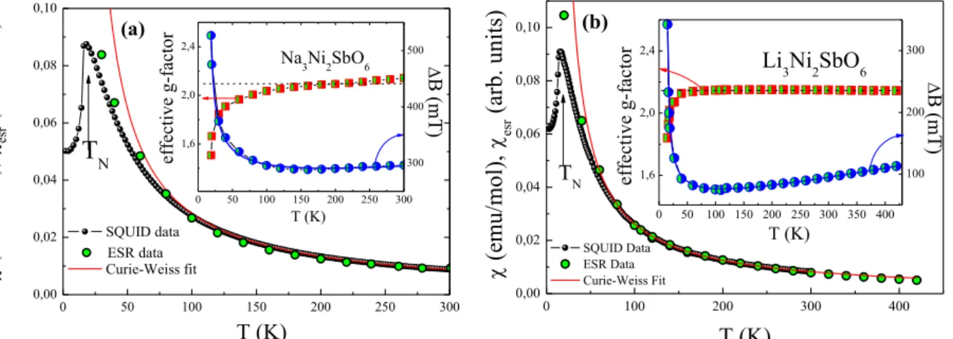
The static and dynamic magnetic properties of A3Ni2SbO6 (A=Li, Na) are similar for both samples and are in full agreement with previously reported data [17,20]. The magnetic susceptibility  = M/B in weak magnetic fields passes through sharp maxima at T ~ 15 and 17 K for Li and Na samples, respectively, then it drops by about one third (Fig. 3). Such a behavior indicates an onset of antiferromagnetic long-range ordering in the material at low temperature and is typical for polycrystalline easy-axis antiferromagnets.

The high temperature magnetic susceptibility nicely follows the Curie-Weiss law with addition of a temperature-independent term 0:

    T C 0   (1)

where  is the Weiss temperature, C is the Curie constant C = NAeff2B2/3kB, NA is Avogadro’s number, eff is the effective magnetic moment, B is Bohr’s magneton, and kB is Boltzmann’s constant. The best fitting according to Eq. 1 in the range 200 – 300 K resulted in positive 0 ~ 1 10-4 emu/mol, which appears to indicate a predominance of the Ni2+ van Vleck paramagnetic contribution over diamagnetic contributions. Our analysis yields positive values for the Weiss temperature: ~ 8 K for Li sample and ~12 K for Na sample, respectively, suggesting the existence of non-negligible ferromagnetic couplings, although the system orders antiferromagnetically at low temperatures. The effective magnetic moments determined from the corresponding Curie constants were found to be 4.3 and 4.4 B/f.u. for Li3Ni2SbO6 and Na3Ni2SbO6 respectively. These values agree well with theoretical estimates theor2

=g2B2nS(S+1), where n is number of Ni2+ ions per formula unit, using an effective g-value

~2.15 and assuming Ni2+ in a high-spin configuration (S=1). In an applied magnetic field the maximum of the magnetization M(T) broadens (not shown), and slightly shifts towards low-temperatures with increasing magnetic field as one would expect in the presence of antiferromagnetic ordering.

B. Electron spin resonance

ESR data in the paramagnetic phase (T>TN) show a single broad Lorentzian shape line ascribable to Ni2+ ions in octahedral coordination. The main ESR parameters (effective g-factor, the ESR linewidth and the integral ESR intensity) were deduced by fitting experimental spectra with asymmetric Lorentzian profile [45] taking into account a small contribution of the dispersion into absorption and two circular components of the exciting linearly polarized microwave field on both sides of B = 0,

 

 





where P is the power absorbed in the ESR experiment, B the magnetic field, Br the resonance field, and B the linewidth.  denotes the asymmetry parameter, which is the fraction of the dispersion added to the absorption. The admixture of dispersion to the absorption signal is usually observed in metals. Here, we are dealing with an insulator, in which the asymmetry arises from the influence of non-diagonal elements of the dynamic susceptibility. This effect is often observed in systems with interactions of low symmetry, geometrical frustration and sufficiently broad resonance lines (Br  B) [46-49].

The overall temperature behavior of the ESR parameters agrees very well for both samples. The integral ESR intensity esr, which is proportional to the number of magnetic spins, was estimated by double integration of the first derivative ESR spectrum dP/dB. It is shown in

Fig. 3 along with static susceptibility data for comparison. One can see that esr follows the Curie-Weiss relationship and agrees well with behavior of  for both compounds. The average effective g-factor g=2.150.03 remains almost temperature independent in the paramagnetic phase down to ~ 140 K for Na sample and ~ 70 K for Li one, then the visible shift of the resonant field to higher magnetic fields begins upon approaching the Néel temperature. This behavior implies the presence of strong short-range correlations in the compound at temperatures noticeably higher than TN, which is frequently characteristic of the systems with a frustration and lower dimensionality [50,51], and the range of these correlations is apparently wider for Na sample. Remarkably that the ESR signal for Na3Ni2SbO6 sample is at least twice broader than for Li3Ni2SbO6 (insets in Fig. 3) and as a consequence the asymmetry parameter takes appreciable value  ~0.4 for sodium compound, while it is negligibly small  ~ 0 for lithium sample. Note, that the value  = 0 leads to a symmetric Lorenzian line, whereas the value  = 1 gives an asymmetric resonance line with absorption and dispersion at equal strength.

The linewidth decreases weakly and almost linearly upon lowering of the temperature, passes through minimum at ~ 140 K for Na sample and ~ 120 K for Li one and eventually changes the trend. Upon further decrease of the temperature the absorption line broadens significantly and the ESR signal vanishes in the vicinity of the Néel temperature, indicating an opening of the energy gap for resonance excitations, e.g., due to the establishment of AFM order. The broadening of the ESR line may be treated in terms of critical behavior of ESR linewidth due to slowing down of spin fluctuations in the vicinity of order-disorder transition [52-55]. This causes the divergence of the spin correlation length, which in turn affects the spin-spin relaxation time of exchange narrowed ESR lines resulting in the critical broadening. To account the B behavior over the whole temperature range we have also included the third linear term into the fitting formula:

 

where the first term B* describes the exchange narrowed linewidth, which is temperature independent, while the second term reflects the critical behavior with TNESR being the temperature of the order-disorder transition and  is the critical exponent. Solid blue lines on insets on Fig. 3 represent a least-squares-fitting of the B(T) experimental data in accordance with Eq. 3. The best fitting was attained with the parameters listed in Table I.

TABLE I. The parameters yielded from fitting of temperature dependencies of the ESR

linewidth B in accordance with Eq. 3 for Na3Ni2SbO6 and Li3Ni2SbO6.

TNESR (K) B* (mT) A (mT) C (mT/K)  (K)

Na3Ni2SbO6 151 2305 1305 0.12 0.50.1

Li3Ni2SbO6 131 255 955 0.18 0.80.1

Here, it is worth the mention two important issues following from the analysis of the linewidth behavior. Firstly, the main experimental feature of B temperature evolution, that the linewidth passes through a minimum as T is decreased, is to be contrasted with that of a 3D system, when the linewidth usually varies approximately as B(T) ~ (T)-1 _{achieving the} temperature-independent high-temperature limit B* associated with the contribution of anisotropic spin-spin interactions in exchange-narrowed regime since in three dimensions the sum over all wave vectors q tends to be weakly dependent on T [56]. At the same time as it has been shown by Richards and Salamon [56] if the most of the contribution comes from q = 0, as is the case in two dimensions, one should expect B(T) ~ (T)1. Moreover, since the relative strength of q  0 modes is decreased with lowering temperature, it follows that the anisotropy will also decrease. Indeed, such behavior was experimentally observed for the plenty of 2D antiferromagnets [57-65] and linear dependence of the B was usually associated either with phonon modulation of the anisotropic and antisymmetric exchange interactions with the magnitude of the dependence proportional to intralayer exchange parameter J4 or with the crystalline field, the latter for S > ½ case. For transition metals where the orbital contribution to the ground state is severely quenched, the latter interactions are rather small and give rise to

d(B)/dT usually smaller or equal 0.1 mT/K. In present case, however, the rate is a bit larger

indicating the noticeable role of the orbital contribution for Ni2+ ions.

The second point to note is that in the framework of Kawasaki approach [52,53], the absolute value of critical exponent can be expressed as  = [(7 + )/22(1  )], where  describes the divergence of correlation length,  is a critical exponent for the divergence of static correlations, and  reflects the divergence of the specific heat. Using the values  =  = 0 and  = 2/3 for 3D antiferromagnets in the framework of the Heisenberg model,  becomes 1/3, which is obviously lower than our experimental values

Both the above mentioned conclusions, following from the analysis of spin dynamics, support the picture of rather 2D character of magnetic correlations in Na3Ni2SbO6 and Li3Ni2SbO6 compounds and well compatible with spin-configuration model, which we suggest based on density functional calculations (see below).

0 50 100 150 200 250 300 0,00 0,02 0,04 0,06 0,08 0,10 SQUID data Curie-Weiss fit T_N  (emu /mo l),  esr (arb. u nit s) T (K) (a) 0 50 100 150 200 250 300 1,6 2,0 2,4 T (K) ef fe cti ve g-f ac tor _Na 3Ni2SbO6 ESR data 300 400 500  B (m T ) 0 100 200 300 400 0,00 0,02 0,04 0,06 0,08 0,10  (emu /mo l),  esr (arb. u nit s) (b)  B (m T) SQUID Data ESR Data Curie-Weiss Fit T (K) T_N 0 50 100 150 200 250 300 350 400 1,6 2,0 2,4 Li₃Ni₂SbO₆ eff ec tive g-f ac tor T (K) 100 200 300

FIG. 3. Temperature dependence of magnetic susceptibility at B = 0.1 T (black filled circles) and

curves represent an approximation in accordance with the Curie-Weiss law. Insets: Temperature dependences of the effective g-factors (half-field squares) and ESR linewidths (half-fieled circles) for both compounds. The blue solid curves on insets represent the result of fitting in the frame of modified Huber theory as described in the text.

C. Magnetization

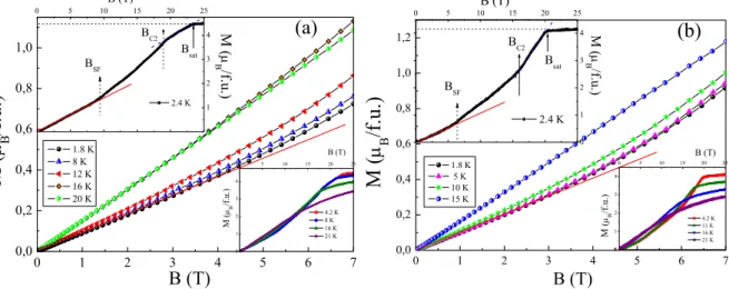
The magnetization isotherms M(B) in static up to 7 T and in pulsed up to 25 T magnetic fields for Na3Ni2SbO6 and Li3Ni2SbO6 at various temperatures are presented in Fig. 4. We observe that the full saturation of the magnetic moment is achieved at about Bsat ~ 23 and 20 T for Na3Ni2SbO6 and Li3Ni2SbO6, respectively, and Msat is in good agreement with the theoretically expected saturation magnetic moment for two high-spin Ni2+ ions (S=1) per formula unit assuming a state: Ms 2gSB = 4.3 B/f.u. (see upper insets in Fig. 4). In addition,

the magnetization curves demonstrate a clear upward curvature suggesting the presence of a magnetic field induced spin-flop type transition in the compounds with the critical fields BSF ~ 9.8 and 5.5 T for Na3Ni2SbO6 and Li3Ni2SbO6, respectively. Moreover, further increase of the magnetic field leads to another change in curvature of the magnetization curves at about BC2 ~ 18 for Na3Ni2SbO6 and BC2 ~ 15 T for Li3Ni2SbO6 indicating the presence of one more magnetic field induced phase transition, that is perhaps related to additional spin reorientation in applied fields. With increasing temperature, both BSF and BC2 anomalies slightly shift to lower fields, weaken in amplitude, and eventually disappear above the Néel temperature TN (see lower insets in Fig. 4). The similar behavior was reported for several other structurally related honeycomb compounds recently. In particular two spin-reorientation transitions below Neel temperature were revealed for Na3Ni2BiO6 [33] and for both 2H and 3R polytypes of Cu3Co2SbO6 [31,66]. Remarkably, the magnetic structure as refined experimentally from low temperature neutron diffraction studies was described as alternating ferromagnetic chains coupled antiferromagnetically giving overall antiferromagnetic zigzag alignment for both Na3Ni2BiO6 (with propagation vector q=[010]) and 2H polytype of Cu3Co2SbO6 (with propagation vector q=[100]). 0 1 2 3 4 5 6 7 0,0 0,2 0,4 0,6 0,8 1,0 B (T) M (  B /f .u.) 1.8 K 8 K 12 K 16 K 20 K (a) 0 1 2 3 4 0 5 10 15 20 25 B (T) M ( B /f .u. ) 4.2 K 8 K 16 K 21 K 0 5 10 15 20 25 0 1 2 3 4 2.4 K M (  B_/f.u.) B (T) B_sat B_C2 B_SF 0 1 2 3 4 5 6 7 0,0 0,2 0,4 0,6 0,8 1,0 1,2 (b) 1.8 K 5 K 10 K 15 K M (  B /f.u.) B (T) 0 1 2 3 4 0 5 10 15 20 25 4.2 K 11 K 16 K 21 K B (T) M ( B /f .u. ) 0 5 10 15 20 25 0 1 2 3 4 B_sat B_C2 B_SF 2.4 K M (  B_/f. u.) B (T)

FIG. 4. The magnetization isotherms in static and pulsed (insets) magnetic fields for

Na3Ni2SbO6 (a) and Li3Ni2SbO6 (b) at various temperatures. Arrows point the positions of the field-induced phase transitions.

D. Specific heat

In order to analyze the nature of the magnetic phase transition and to evaluate the corresponding contribution to the specific heat and entropy, the structurally similar [7] diamagnetic material Li3Zn2SbO6 has been synthesized. The specific heat data for both magnetic and diamagnetic samples in the T-range 2-300 K are shown in Fig. 5. The Dulong-Petit value reaches 3Rz = 299 J/mol K, with the number of atoms per formula unit z = 12. The C(T) data for

A3Ni2SbO6 (A=Li, Na) in zero magnetic field are in good agreement with the temperature dependence of the magnetic susceptibility in weak magnetic fields, and demonstrate a distinct -shaped anomaly, which is characteristic of a 3D magnetic order (Fig. 5). Note, that the absolute value of the Néel temperature TN ~ 14 and 16 K for Li3Ni2SbO6 and Na3Ni2SbO6 respectively, deduced from C(T) data at B = 0 T is slightly lower than the Tmax in (T) at B = 0.1 T (Fig. 3), whereas it correlates well with a maximum on the magnetic susceptibility derivative /T(T). Indeed, as has been shown by Fisher [67,68] that the temperature dependence of the specific heat

C(T) for antiferromagnets with short-range interactions should follow the derivative of the

magnetic susceptibility in accordance with:

 

 



 



C  _ _|| (4)

where the constant A depends weakly on temperature. In accordance with Eq. (2), the -type-anomalies observed in C(T) dependence at the antiferromagnetic transition temperature are defined by an infinite positive gradient on the curve (T) at TN, while a maximum (T) usually lies slightly above the ordering temperature. Thus, the anomaly in the specific heat should correspond to the similar anomaly in /T(T) [69].

We observe a specific heat jump at TN Cp ~ 32 J/mol K and 33 J/mol K for Li3Ni2SbO6 and Na3Ni2SbO6, respectively, which are only slightly smaller than the value expected from the mean-field theory for the antiferromagnetic ordering of two Ni2+ ions system assuming all spins

to be in the high-spin (S=1) state [70]:









C_p  33.2 J/(mol K), where R is the

gas constant R=8.31 J/mol K. In applied magnetic fields, the TN - anomaly is rounded and markedly shifts to lower temperatures (see insets in Fig. 5).

For quantitative estimations we assume that the specific heat of the isostructural compound Li3Zn2SbO6 provides a proper estimation for the pure lattice contribution to specific heat. In the frame of the Debye model the phonon specific heat is described by the function [70]:







where x =ħ/kBT, D = ħmax/kB is the Debye temperature, max is the maximum frequency of

the phonon spectrum and kB is the Boltzmann constant. The value of the Debye temperature D estimated from approximating C(T) to this T3 – law in the low temperature range for the diamagnetic compound Li3Zn2SbO6 was found to be about ~ 515  5 K. Normalization of the Debye temperatures has been made taking into account the difference between the molar masses for Zn – Ni and Li – Na atoms in the A3Ni2SbO6 compounds resulting in D ~ 5235 K and 4155 K for Li and Na samples, respectively.

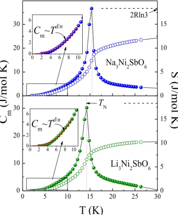
The magnetic contribution to the specific heat was determined by subtracting the lattice contribution using the data for the isostructural non-magnetic analogue [7] (Fig. 6). We examine the Cm(T) below TN in terms of the spin-wave (SW) approach assuming that the limiting low-temperature behavior of the magnetic specific heat should follow a Cm  Td/n - power law due to magnon excitations [50], where d stands for the dimensionality of the magnetic lattice and n is defined as the exponent in the dispersion relation  ~ n. For antiferromagnetic (AFM) and ferromagnetic (FM) magnons n = 1 and n = 2, respectively. The least square fitting of the data below TN (insets in Fig. 6) agrees well with d = 3 and n = 1 for both Li and Na samples, what corroborates the picture of 3D AFM magnon excitations at low temperatures.

In Fig. 6 we also show the entropy change (open circles) in both materials calculated using the equation: 

 



 

m dT T T C T S 0

. We observe that the magnetic entropy Sm saturates at temperatures higher than 25 K, reaching approximately 10-12 J/(mol K). This value is definitely lower than the magnetic entropy change expected from the mean-field theory for a system of two

nickel magnetic ions with S=1: S_m

 





0 50 100 150 200 250 300 0 50 100 150 200 250 300 C p (J/mo l K) Na₃Ni₂SbO₆ Li₃Zn₂SbO₆ Li₃Ni₂SbO₆ T (K) 3R= 299 J/mol K T_N 0 10 20 30 40 4 6 8 10 12 14 16 18 Li₃Ni₂SbO₆ Cp ( J/ m ol K) T (K) 9T 6T 3T 0T (b) 6 8 10 12 14 16 0 10 20 30 40 Na₃Ni₂SbO₆ C p ₍ J/ m ol K) T (K) 9T 7T 5T 3T 0T (a)

FIG. 5. Temperature dependence of the specific heat in Li3Ni2SbO6 (green triangles), Na3Ni2SbO6 (blue filled circles) and their non-magnetic analogue Li3Zn2SbO6 (black half-filled circles) in zero magnetic field. Insets: enlarged low temperature parts highlights the onset of antiferromagnetic spin ordering and shift of the TN in magnetic fields.

0 10 20 30 Na₃Ni₂SbO₆ 2Rln3 0 5 10 15 20 25 30 0 10 20 30

S

(J/mol

K

)

C

(J/mol

K

)

T (K)

C

~T

C

~T

FIG. 6. Magnetic specific heat (filled circles) and magnetic entropy (open circles) for

A3Ni2SbO6 at B=0 T. Insets: enlarged low temperature parts with solid curve indicating the spin wave contribution estimated in accordance with Cm  Td/n - power law for magnons.

E. Nuclear magnetic resonance

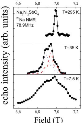
The typical 23Na field-dependent NMR spectrum of Na3Ni2SbO6 at room temperature contains a narrow main line and quadrupole satellites (Fig. 7). Upon decreasing the temperature the spectrum broadens noticeably and shifts to the lower field side. The temperature behavior of

the spectrum of Li3Ni2SbO6 (not shown) is similar to the data for Na3Ni2SbO6. However, the quadrupole moment of Li nuclei is almost 10 times smaller than Na, so that the room temperature spectrum of Li3Ni2SbO6 does not contain the well-resolved satellites.

Both spectra of Na3Ni2SbO6 and Li3Ni2SbO6 are inhomogeneously broadened and consist of two components, which can be attributed to two crystallographically [39] and magnetically nonequivalent positions of alkali metal ions. An example of the spectrum decomposition in Na3Ni2SbO6 in accordance with the two resolved components is shown in the middle panel of

Fig. 7.

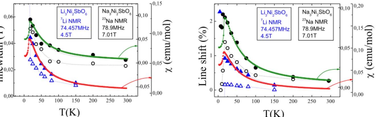
The temperature dependence of the lineshift and linewidth of Na and Li signals are collected in Fig. 8. Obviously, their behavior agrees well with the corresponding evolution of the magnetic susceptibility below ~200 K.

The low-temperature behavior of the NMR spectrum is caused by the interaction with the magnetic Ni2+ ions and reflects the dynamics of magnetic subsystem. The fact that the shift and broadening of the lines start at much higher temperatures than TN indicates the existence of strong low-dimensional (short-range) correlations in the magnetic subsystem [50,71]. The slowing down of the Ni magnetic moments fluctuations caused by competing ferro- and antiferromagnetic interactions in the planes with much weaker interplane couplings, as determined from DFT calculations (see next subsection), creates a non-zero average magnetic field at the Na/Li nuclei situated in between the Ni-Sb planes.

6,6 6,8 7,0 7,2 6,6 6,8 7,0 7,2 T=7.5 K T=295 K Na₃Ni₂SbO₆ 23 Na NMR 78.9MHz

Field (T)

ec

ho inte

nsi

ty (a

rb. units

)

FIG. 7. The 23Na NMR spectrum at various temperatures. Dashed lines are the fitted contributions of two sodium sites, solid line is the best fit of the spectra.

The hyperfine tensor value is different for different Na/Li positions and hence it can explain the different values of Knight shifts and linewidths of the spectral components. Another possible explanation of the asymmetric shape of powder NMR spectra, i.e. strong hyperfine tensor asymmetry, seems to us less probable because the ratio of the intensity of the components in both compounds is about 1:1 and the spectrum does not fit to the typical powder lineshape. One should mention that the ESR data do not give an evidence for the existence of a strong g-factor anisotropy which also could contribute to the anisotropy of the average field on the position of the alkali metals nuclei. Nevertheless, the ESR absorption line for sodium compound was found to be essentially wider than for lithium one, that indicates larger anisotropy for sodium compound. It is worth to note that both the NMR lineshift and the NMR linewidth for

Na3Ni2SbO6 are also markedly larger than for Li3Ni2SbO6 even taking into account the field dependence of the inhomogeneously broadened NMR line. This fact is likely to manifest the features of two different magnetic subsystems of these compounds: the ionic radius of Na is essentially larger than Li one and leads to enlarged distances between magnetically-active (Ni2SbO6) layers and as a consequence to a weaker exchange coupling between them in Na3Ni2SbO6.

The NMR lineshape of the sodium and lithium spectra undergoes significant changes upon approaching the Neel temperatures (at about T ~ 17 К and T ~ 15 К for sodium and lithium compounds, respectively) indicating the onset of long-range magnetic order when the sublattice of nickel magnetic ions creates a static local field at the alkali metal positions. Na/Li positions are almost symmetrical relative to the two magnetic honeycomb planes. In such cases the magnitude of the local field is small enough [72] and the total width of the spectra is about 0.2 – 0.35 T depending on the external magnetic field.

We should note that the external magnetic fields range in both cases (4.5 T for 7Li and 7.01 T for 23Na) corresponds to the developing of the spin-flop phase (compare with BSF which are about 5.5 T and 9.8 T for Li3Ni2SbO6 and Na3Ni2SbO6 as described above). The differences of the internal field distribution and magnitude at different magnetic fields are exemplified by the NMR spectrum of 7Li (Fig. 9) obtained in relatively large (4.5 T) and small (0.95 T) external fields. 0 50 100 150 200 250 300 0,00 0,02 0,04 0,06 -0,05 0,00 0,05 0,10 0,00 0,05 0,10 0,15  (em u/mol) Na₃Ni₂SbO₆ 23_{Na NMR} 78.9MHz 7.01T Li₃Ni₂SbO₆ 7_{Li NMR} 74.457MHz 4.5T T(K) linewid th (T) 0 50 100 150 200 250 300 0 1 2 0,00 0,05 0,10 0,00 0,05 0,10 0,15 0,20  (em u/mol) Li₃Ni₂SbO₆ 7_{Li NMR} 74.457MHz 4.5T Line sh ift ( %) T(K) Na₃Ni₂SbO₆ 23_{Na NMR} 78.9MHz 7.01T

FIG. 8.The temperature dependencies of linewidth (left) and line shift (right) of two components

of 7Li (triangles, blue online) and 23Na (circles, black online) NMR signals. Dotted lines are guides for eyes. Small red and green circles are the magnetic susceptibility curves.

The local fields on the lithium positions at the external field = 0.95 T was calculated in the frame of the dipole-dipole model assuming an isotropic hyperfine tensor [73]. The quadrupole splitting and inhomogeneous line broadening were not taken into account. The calculation includes only 16 nearest neighbor Ni ions in a sphere of radius 5.2 Å, the powder averaging of the internal magnetic field was made according to Ref. 74. The calculations in the frame of different models, mentioned in Fig. 1 have been performed and we have found that the most part of the models cannot explain the complicated structure of the spectrum. The best fit of the experimental data (as shown by a red dashed curve in Fig. 9) was obtained assuming a zigzag spin structure with spins oriented perpendicular to the plane. For the sake of better description of experimental data we also included into fitting model the Gaussian contribution from the Li-positions situated close to structure defects. It can be shown that the Li Li-positions with a minimal local field are the most affected by in-plane defects so the transfer of the spectral intensity from these “regular” to “defect” component is expected. At 4.5 T we have a smooth spectra shape due to the partial flipping of the spins while developing the spin-flop phase. The proper fitting of the 4.5T spectrum was impossible because of the spin-flop transition is not finally occurred at that field (as it was mentioned above BSF ~ 5.5 T for Li sample). But on the base of our calculations one can expect comparably narrow rectangular-like spectrum in the spin-flop phase. To verify the magnetic structure in the spin-flop phase the high-field NMR experiments might probably be

useful, but they were beyond of the scope of this work. In the next section we show that the critical field, at which the spin flop phase appears, agrees reasonably with density functional theory estimations.

F. Density functional theory determination of exchange interactions

In Fig. 10 we present the electronic structure of Na3Ni2SbO6 in the generalized gradient approximation (GGA) in the energy range [-2eV, 0.5eV] around the Fermi level. There are ten bands of predominant Ni character, originating from the 3d bands of the two Ni ions in the primitive cell used for the calculation. This band manifold is 4/5th filled since in Na3Ni2SbO6 nickel is in the Ni2+ (3d8) oxidation state and antimony in the Sb5+ state (filled shell). The distorted octahedral environment of Ni, NiO6, leads to a t2g - eg splitting of about 1.5 eV. The

three t2g states 3dxy, 3dyz and 3dxz are completely filled (see the density of states (DOS)) and the

eg states 3dz2 and 3dx2-y2 are half-filled. Thus, we expect Ni to be in a high spin state with S = 1 in

Na3Ni2SbO6. Indeed, spin polarized GGA calculations show that Ni favors moments of 2 µB for both compounds. The electronic structure of Li3Ni2SbO6 (not shown) is similar to that of Na3Ni2SbO6. 4,0 4,2 4,4 4,6 4,8 5,0 0,4 0,6 0,8 1,0 0,2 0,4 0,6 0,8 1,0 0,4 0,6 0,8 1,0 1,2 1,4 1,6 7 Li-NMR 74.457 MHz 4.2 K Field (T)

echo intensity (arb. units)

Field (T)

7_Li-NMR

15.79 MHz 4.2 K

FIG.9. The 7Li spectrum for Li3Ni2SbO6 at 4.2 K in AFM phase at different magnetic fields: 0.95 T for upper panel and 4.5 T for lower panel. Red line is the result of dipole-dipole calculations, dashed lines are the calculated contributions of different magnetically non-equivalent lithium positions in frame of the powder averaging of zigzag model .

Both systems are insulators, consideration of zigzag magnetic order in the calculations opens a gap in the electronic structure of about 1.5 eV. Including correlation effects as implemented in GGA+U and for a value of U - J = 4 eV which is reasonable for 3d electrons, we obtain a charge gap of 2.77 eV. A refinement of this choice will be discussed below. Measurements of the charge gap will be desirable but are beyond the scope of the present work.

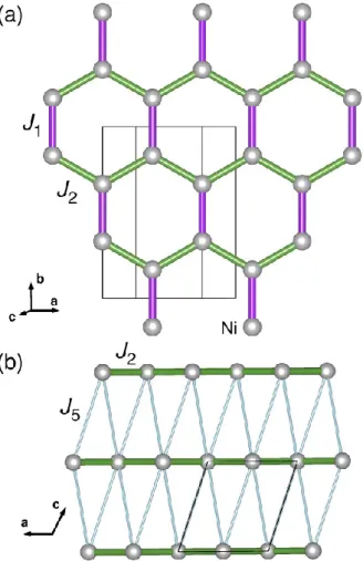
We now proceed to analyze the magnetic interactions in Na3Ni2SbO6 and Li3Ni2SbO6. In order to obtain the magnetic couplings we performed total energy calculations for different spin configurations within GGA and GGA+U and mapped their differences to a Heisenberg model. Total energy differences between spin configurations for the four Ni sites in the conventional unit cell with symmetry lowered to P1 yield the first three exchange couplings given in Table II for Na3Ni2SbO6 (converged on an 8x8x8 k mesh). J3 is a second nearest neighbor coupling within the hexagon and turns out to be quite small. The nearest neighbor coupling J1 is

antiferromagnetic and strongly depends on the value of U in the GGA+U calculation. The next nearest neighbor coupling J2 is ferromagnetic and is nearly independent of U. The pattern is shown in Fig. 11. The ratio |J1/J2| thus depends on the question which U better describes the material. As mentioned above, the average charge gap at U - J = 4 eV is 2.77 eV, at U - J = 6 eV is 2.96 eV. We note that the present calculations clearly favor a zigzag magnetic order of Ni; the

zigzag magnetic order also has the lowest energy of all four spin configurations considered. Zigzag order is 2.4 meV per formula unit lower in energy than ferromagnetic order at U - J = 4.5

eV. A 1x1x2 supercell was used to estimate the order of magnitude of interlayer exchange couplings and given as J5 [75] in Table II. In order to decide which value of U is the best for Na3Ni2SbO6 and Li3Ni2SbO6, we calculated the magnetic susceptibilities using 10th order high temperature series expansion (HTE10) [76]. From comparison with the experimental susceptibility in Fig. 3, we have found that U - J = 4.5 eV is the best choice. The corresponding set of the exchange couplings for Li3Ni2SbO6 is given also in Table II. Note that due to the smaller inter-layer distance in Li3Ni2SbO6, the order of nearest neighbor distances is reversed.

Thus, the present DFT results allow us to compare the magnetic Hamiltonians of Na3Ni2SbO6 and Li3Ni2SbO6. The intralayer couplings J1 and J2 are slightly larger in the Li system than in the Na system due to the shorter Ni-Ni distances in the Li system. The most significant difference is the slightly more 3D character of Li3Ni2SbO6 as seen in the somewhat larger interlayer couplings. This is plausible as the smaller Li ions lead to a smaller c lattice parameter and thus a smaller separation between the honeycomb layers.

Finally, we have performed fully relativistic spin polarized calculations for Na3Ni2SbO6 in order to estimate the importance of spin orbit coupling and determine the easy axis for the Ni spins and the corresponding magnetocrystalline anisotropy. We have found that the lowest energy is obtained by orienting the quantization axis along c*, perpendicular to the honeycomb layers. In-plane energies are 0.067 meV/formula unit (a axis) and 0.072 meV/formula unit (b axis) higher in energy. This estimate agree with the calculated anisotropy energies using VASP: we obtain in-plane energies 0.088 meV/formula unit (a axis) and 0.065 (b axis) higher than the out-of-plane case. Therefore, the spins tend to align perpendicularly to the honeycomb layers in agreement with the suggestion from NMR experiments (see previous section).

Using the approximation of Ref. 77, we estimate the value of the spin flop field BSF as

BSF = 2√KΔ/M, where K is the magnetocrystalline anisotropy energy, Δ=2.4 meV/f.u. is the energy difference between ferromagnetic and zigzag antiferromagnetic states, and M is the Ni magnetic moment. We find a spin flop field of BSF = 7.2 Tesla for Na3Ni2SbO6 which underestimates the experimental value but remains qualitatively of the same order of magnitude. The estimation for a spin-flip (saturation) field gives about 20 T in good agreement with experimentally found value Bsat ~ 23 T.

TABLE II. Exchange couplings of Na3Ni2SbO6 and Li3Ni2SbO6 (in Kelvin) calculated with GGA+U at U = 5.5 eV, J = 1 eV. J3 is a second nearest neighbor coupling across a hexagon, J5 is a coupling along c between the honeycomb layers.

J1 (K) J2 (K) J3 (K) J5 (K)

Na3Ni2SbO6 15 -22 0 1

FIG. 10. Band structure and density of states of Na3Ni2SbO6. Partial densities of states for the Ni 3d orbitals are also shown.

FIG. 11. Important exchange paths of Na3Ni2SbO6. (a) The purple nearest neighbor coupling J1 is antiferromagnetic, the green next nearest neighbor coupling J2 is ferromagnetic. (b) There is a small antiferromagnetic coupling J5 between the honeycomb Ni planes (light blue).

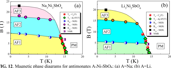
G. Magnetic phase diagrams

Summarizing the data, the magnetic phase diagrams for the new layered antimonates A3Ni2SbO6 can be suggested (Fig. 12). At temperatures above TN in zero magnetic field the paramagnetic phase is realized. With increasing the magnetic field this phase transition boundary shifts slowly to lower temperature side. The antiferromagnetic state, however, is complicated by presence of two more field-induced phases at low temperatures. The quantum ground state determined as zigzag antiferromagnetic state (AF1) exists below 5 T for Li3Ni2SbO6 and 10 T for Na3Ni2SbO6 compound, respectively. The field-induced spin-flop phase (AF2) was found to be realized in the field ranges 5 - 15 T for Li3Ni2SbO6 and 10 - 18 T for Na3Ni2SbO6 and those are replaced by another field-induced antiferromagnetic phase (AF3) which most probably is corresponding to another spin configuration. The spin-flip transition is realized at 20 and 23 T for Li3Ni2SbO6 and Na3Ni2SbO6 compound, respectively. These observations are well accounted for by density functional calculations for the main magnetic exchange interactions, which show that the both antiferromagnetic and ferromagnetic intralayer spin exchanges are present on the honeycomb planes resulting in zigzag antiferromagnetic ground state on honeycomb lattice. The neutron scattering studies in applied magnetic fields would be desirable for determination of actual spin-configurations in AF1, AF2 and AF3 phases.

0 5 10 15 20 0 5 10 15 20 25 AF3 AF1

(a)

B

(T)

T (K)

B

(T)

T (K)

(b)

FIG. 12. Magnetic phase diagrams for antimonates A3Ni2SbO6: (a) A=Na; (b) A=Li.

IV. Conclusion

In conclusion, we have examined the thermodynamic and resonance properties of two layered honeycomb-lattice monoclinic oxides A3Ni2SbO6 (A=Li, Na) by both bulk (magnetic susceptibility, magnetization and specific heat) and local (ESR and NMR) experimental techniques and by performing density functional theory calculations. The overall results are consistent with each other and yield the picture of a complex magnetic ordering at low temperatures. Magnetic susceptibility and specific heat data indicate the onset of antiferromagnetic long range order. In addition, the magnetization curves reveal a field-induced (spin-flop type) transition below TN that can be understood in terms of the magnetocrystalline anisotropy in these systems. ESR and NMR show the presence of appreciable low-dimensional (short-range) correlations below ~ 100 K. The theoretical calculations have shown that interplane exchange coupling is very weak for both compounds, so that they both can be considered as 2D magnets. At the same time both ferromagnetic and antiferromagnetic intraplane exchange interactions are present on the honeycomb Ni2SbO6 layers and the most favorable spin configuration model is zigzag ferromagnetic chains coupled antiferromagnetically. This magnetic configuration is well compatible with our NMR data.

Acknowledgments

The work was supported by the Russian Foundation for Basic Research (grants 11-03-01101 for E.A.Z. and V.B.N., 14-02-00245 for E.A.Z., E.L.V and M.I.S., 14-02-01194 for E.L.V and M.F.I.). The work of M.A. and A.V.S. was supported by the FNRS projects, crédit de démarrage U.Lg. M.A. thanks Jun Li (INPAC – K. U. Leuven) for assistance in measurements and H-L. Feng, K. Yamaura (National Institute for Materials Science, Japan) for discussion of specific heat data. H.O.J. and R.V. thank the Deutsche Forschungsgemeinschaft (DFG) for financial support through SFB/TR49. A.N.V. acknowledges support from the Ministry of Education and Science of the Russian Federation in the framework Increase Competitiveness Program of NUST «MISiS» (№ К2-2014-036). The authors thank L.I. Medvedeva and M.A. Evstigneeva for providing samples used in present work.

References

1. B. Xu, D. Qian, Z. Wang, Y.S. Meng, Mater. Sci. Eng. R 73, 51 (2012). 2. J.B. Goodenough, J. Solid State Electrochem. 16, 2019 (2012).

3. I. Terasaki, Y. Sasago, K. Uchinokura, Phys. Rev. B 56, R12685 (1997).

4. M. Lee, L. Viciu, L. Li, Y. Wang, M.L. Foo, S. Watauchi, R.A. Pascal Jr., R.J. Cava, N.P. Ong, Nat. Mater. 5, 537 (2006).

5. K. Takada, H. Sakurai, E. Takayama-Muromachi, F. Izumi, R.A. Dilanian, T. Sasaki,

Nature 422, 53 (2003).

6. J. D. Jorgensen, M. Avdeev, D. G. Hinks, J. C. Burley, S. Short, Phys. Rev. B 68, 214517 (2003).

7. C. Greaves, S.M.A. Katib, Mater. Res. Bull. 25, 1175 (1990).

8. G.C. Mather, C. Dussarrat, J. Etourneau, A.R. West, J. Mater. Chem. 10, 2219 (2000). 9. R. Nagarajan, S. Uma, M.K. Jayaraj, J. Tate, A.W. Sleight, Solid State Sci. 4, 787 (2002). 10. J. Xu, A. Assoud, N. Soheilnia, S. Derakhshan, H.L. Cuthbert, J.E. Greedan, M.H.

Whangbo, H. Kleinke, Inorg. Chem. 44, 5042 (2005).

11. S. Derakhshan, H.L. Cuthbert, J.E. Greedan, B. Rahaman, T. Saha-Dasgupta, Phys. Rev.

B 76, 104403 (2007).

12. Y. Miura, R. Hirai, Y. Kobayashi, M. Sato, J. Phys. Soc. Japn. 75, 084707 (2006). 13. Y. Miura, R. Hirai, T. Fujita, Y. Kobayashi, M. Sato, J. Magn. Magn. Mater. 310, 389

(2007).

14. Y. Miura, Y. Yasui, T. Moyoshi, M. Sato, K. Kakurai, J. Phys. Soc. Japn. 77, 104709 (2008).

15. C.N. Kuo, T.S. Jian, C.S. Lue, J. Alloys Comp. 531, 1 (2012).

16. O.A. Smirnova, V.B. Nalbandyan, A.A. Petrenko, M. Avdeev, J. Solid State Chem. 178 1165 (2005).

17. W. Schmidt, R. Berthelot, A.W. Sleight, M.A. Subramanian, J. Solid State Chem. 201, 178–185 (2013).

18. R. Berthelot, W. Schmidt, A.W. Sleight, M.A. Subramanian, J. Solid State Chem. 196, 225–231 (2012).

19. L. Viciu, Q. Huang, E. Morosan, H.W. Zandbergen, N.I. Greenbaum, T. McQueen, R.J. Cava, J. Solid State Chem. 180, 1060 (2007).

20. E.A. Zvereva, M.A. Evstigneeva, V.B. Nalbandyan, O.A. Savelieva, S.A. Ibragimov, O.S. Volkova, L.I. Medvedeva, A.N. Vasiliev, R. Klingeler, B. Buechner, Dalton Trans.

41, 572 (2012).

21. R. Berthelot, W. Schmidt, S. Muir, J. Eilertsen, L. Etienne, A.W. Sleight, M.A. Subramanian, Inorg. Chem. 51, 5377 (2012).

22. V.V. Politaev, V.B. Nalbandyan, A.A. Petrenko, I.L. Shukaev, V.A. Volotchaev, B.S. Medvedev, J. Solid State Chem. 183, 684 (2010).

23. M.A. Evstigneeva, V.B. Nalbandyan, A.A. Petrenko, B.S. Medvedev, A.A. Kataev,

Chem. Mater. 23, 1174 (2011).

24. V. Kumar, N. Bhardwaj, N. Tomar, V. Thakral, S. Uma, Inorg. Chem. 51, 10471 (2012). 25. V. Kumar, A. Gupta, S. Uma, Dalton Trans. 42, 14992 (2013).

26. V.B. Nalbandyan, M. Avdeev, M.A. Evstigneeva, J. Solid State Chem. 199, 62 (2013). 27. V.B. Nalbandyan, А.А. Petrenko, M.A. Evstigneeva, Solid State Ionics 233, 7 (2013). 28. E.A. Zvereva, O.A. Savelieva, Ya.D. Titov, M.A. Evstigneeva, V.B. Nalbandyan, C.N.

Kao, J.-Y. Lin, I.A. Presniakov, A.V. Sobolev, S.A. Ibragimov, M. Abdel-Hafiez, Yu. Krupskaya, C. Jähne, G. Tan, R. Klingeler, B. Büchner, A.N. Vasiliev, Dalton Trans. 42, 1550 (2013).

29. J.H. Roudebush, R.J. Cava, J. Solid State Chem. 204, 178-185 (2013).

30. E. Climent-Pascual, P. Norby, N.H. Andersen, P.W. Stephens, H.W. Zandbergen, J. Larsen, R.J. Cava, Inorg. Chem. 51, 557 (2012).

31. J.H. Roudebush, N.H. Andersen, R. Ramlau, V.O. Garlea, R. Toft-Petersen, P. Norby, R. Schneider, J.N. Hay, R.J. Cava, Inorg. Chem. 52, 6083-6095 (2013).

32. A. Gupta, C.B. Mullins, J.B. Goodenough, J. Power Sources 243, 817-821 (2013).

33. E.M. Seibel, J.H. Roudebush, H. Wu, Q. Huang, M.N. Ali, H. Ji, R.J. Cava, Inorg. Chem.

52, 13605 (2013).

34. W. Schmidt, R. Berthelot, L. Etienne, A. Wattiaux, M.A. Subramanian, Mater. Res. Bull.

50, 292 (2014).

35. M. Schmitt, O. Janson, S. Golbs, M. Schmidt, W. Schnelle, J. Richter, H. Rosner, Phys.

Rev. B 89, 174403 (2014).

36. N. Bhardwaj, A. Gupta, S. Uma, Dalton Trans. 43, 12050 (2014).

37. A. Mulder, R. Ganesh, L. Capriotti, A. Paramekant, Phys. Rev. B 81, 214419 (2010). 38. P.H.Y. Li, R.F. Bishop, D.J.J. Farnell, C.E. Campbell, Phys. Rev. B 86, 144404 (2012) 39. J. Ma, S.-H. Bo, L. Wu, Y. Zhu, C.P. Grey, P.G. Khalifah, Chem. Mater. 27, 2387

(2015).

40. K. Koepernik, H. Eschrig, Phys. Rev. B 59, 1743 (1999)

41. J. P. Perdew, K. Burke, M. Ernzerhof, Phys. Rev. Lett. 77, 3865 (1996). 42. G. Kresse, J. Furthmüller, Phys. Rev. B 54, 11169 (1996).

43. K. Foyevtsova, I. Opahle, Yu-Zh. Zhang, H.O. Jeschke, R. Valentí, Phys.Rev. B 83, 125126 (2011)

44. U. Tutsch, B. Wolf, S. Wessel, L. Postulka, Y. Tsui, H.O. Jeschke, I. Opahle, T. Saha-Dasgupta, R. Valentí, A. Brühl, K. Remović-Langer, T. Kretz, H.-W. Lerner, M. Wagner, M. Lang, Nature Comm. 5, 5169 (2014).

45. J.P. Joshi, S.V. Bhat, J. Magn. Res. 168, 284 (2004)

46. H.-A. Krug von Nidda, L.E. Svistov, M.V. Eremin, R.M. Eremina, A. Loidl, V. Kataev, A. Validov, A. Prokofiev, W. Aßmus, Phys. Rev. B 65, 134445 (2002).

47. J.M. Law, P. Reuvekamp, R. Glaum, C. Lee, J. Kang, M.-H. Whangbo, R.K. Kremer,

Phys. Rev. B 84, 014426 (2011).

48. V.B. Nalbandyan, E.A. Zvereva, G.E. Yalovega, I.L. Shukaev, A.P. Ryzhakova, A.A. Guda, A. Stroppa, S. Picozzi, A.N. Vasiliev, M.-H. Whangbo, Inorg. Chem. 52, 11850 (2013).

49. E.A. Zvereva, V.B. Nalbandyan, M.A. Evstigneeva, H.-J. Koo, M.-H. Whangbo, A.V. Ushakov, B.S. Medvedev, L.I. Medvedeva, N.A. Gridina, G.E. Yalovega, A.V.

Churikov, A.N. Vasiliev, and B. Büchner, J. Solid State Chemistry 225, 89 (2015) 50. L.J. de Jongh, A.R. Miedema, Adv. Phys., 23, 1 (1974).

51. J. E. Greedan, J. Mater. Chem. 11, 37 (2001) 52. K. Kawasaki, Prog. Theor. Phys. 39, 285 (1968). 53. K. Kawasaki, Phys. Lett. 26A, 543 (1968).

54. H. Mori, K. Kawasaki, Progr. Theor. Phys. 28, 971 (1962). 55. D.L. Huber, Phys. Rev. B 6, 3180 (1972).

56. P.M. Richards and M.B. Salamon, Phys. Rev. B 9, 32 (1974) 57. R.D. Willett and F. Waldner, J. Appl. Phys. 53, 2680 (1982). 58. R.D. Willett, and R. Wong, J. Magn. Res. 42, 446 (1981). 59. T.G. Castner, Jr. and M. S. Seehra, Phys. Rev. B 4, 38 (1971). 60. T.G. Castner and M. S. Seehra, Phys. Rev. B 47, 578 (1993).

61. M. Heinrich, H.-A. Krug von Nidda, A. Loidl, N. Rogado, and R.J. Cava, Phys. Rev. Lett.

91, 137601 (2003).

62. A. Zorko, F. Bert, A. Ozarowski, J. van Tol, D. Boldrin, A. S. Wills, and P. Mendels,

Phys. Rev. B 88, 144419 (2013).

63. D.L. Huber and M.S. Seehra, J. Phys. Chem. Solids 36, 723 (1975).

64. M.S. Seehra, M.M. Ibrahim, V.S. Babu, and G. Srinivasan, J. Phys.: Condens. Matter 8, 11283 (1996).

65. A. Zorko, D. Arčon, H. van Tol, L.C. Brunel, and H. Kageyama, Phys. Rev. B 69, 174420 (2004).

66. J.H. Roudebush, G. Sahasrabudhe, S.L. Bergman and R.J. Cava, Inorg. Chem. 54, 3203 (2015)

67. M.E. Fisher, Proc. Roy. Soc. (London) A 254, 66 (1960). 68. M.E. Fisher, Phil. Mag. 7, 1731 (1962).

69. R.L. Carlin, Magnetochemistry, Springer-Verlag, Berlin Heidelberg New York Tokyo, 1986.

70. A. Tari, The specific heat of matter at low temperature, Imperial College Press, London, 2003.

71. H. Benner, J.P. Boucher, Spin Dynamics in the Paramagnetic Regime: NMR and EPR in

Two-Dimensional Magnets – “Magnetic Properties of Layered Transition Metal Compounds“ ed. L.J. de Jongh, Springer, Netherlands, 1990, pp 323-378.

72. M. Yehia, E. Vavilova, A. Möller, T. Taetz, U. Löw, R. Klingeler, V. Kataev, B. Büchner, Phys. Rev.B 81, 60414 (2010).

73. C.P. Slichter, Principles of Magnetic Resonance, Springer, 1990. 74. Y. Yamada and A. Sakata, J. Phys. Soc. Jpn. 55, 1751 (1986).

75. Note, however, that the given value actually corresponds to a sum of interlayer couplings

J5 + J6 as more effort would be required to distinguish the interlayer couplings. Considering the size compared to J1 and J2 however, this is not necessary. 76. A. Lohmann, H.-J. Schmidt, J. Richter, Phys. Rev. B 89, 014415 (2014). 77. M.D. Watson, A. McCollam, S.F. Blake, D. Vignolles, L. Drigo, I.I. Mazin, D.

Guterding, H.O. Jeschke, R. Valentí, N. Ni, R. Cava, A.I. Coldea, Phys. Rev. B 89, 205136 (2014).