Joint tasks and cache partitioning for real-time systems

(1)

HAL Id: dumas-00725172

https://dumas.ccsd.cnrs.fr/dumas-00725172

Submitted on 24 Aug 2012

HAL is a multi-disciplinary open access

archive for the deposit and dissemination of sci-entific research documents, whether they are pub-lished or not. The documents may come from teaching and research institutions in France or

L’archive ouverte pluridisciplinaire HAL, est destinée au dépôt et à la diffusion de documents scientifiques de niveau recherche, publiés ou non, émanant des établissements d’enseignement et de recherche français ou étrangers, des laboratoires

Joint tasks and cache partitioning for real-time systems

Brice Berna

To cite this version:

Brice Berna. Joint tasks and cache partitioning for real-time systems. Hardware Architecture [cs.AR]. 2012. �dumas-00725172�

(2)

Universit de Rennes 1 Ecole Normale Suprieur de Cachan

Master Thesis

Encadrante de stage : Isabelle Puaut Equipe ALF

Joint tasks and cache partitioning for

real-time systems

Brice Berna

(3)

1 Introduction

A system is a combination of hardware and software intended to interact with the environment. The system detects events using a set of sensors, and acts on the environment through a set of actuators. Some systems must carry out actions in limited time, in order to timely react to the detection of specific events, or perform an action periodically. These systems are known as real-time systems.

There are two types of real-time constraints: soft real-time constraints and hard real-time constraints. A system with soft real-time constraints is authorized to miss its time constraint occasionally without catastrophic consequences. For example, during the decoding of a video, the decoding of a frame should be finished before the frame is displayed. If the decoding is completed too late, the frame is no longer useful and is discarded. If it only happens occasionally, reading is undisturbed. Instead, hard real-time con-straints cannot be missed without serious consequences. For example, hard real-time systems are used in avionics and aerospace, areas where missing timing constraints can be dangerous for people.

Validating time constraints opens up many research issues. For real-time systems running on single-core processors, the steps are basically: (i) to obtain an overestimation of the worst case execution time of all concurrent activities (tasks) to be executed, (ii) scheduling tasks over time, (iii) check-ing that all executions allowed by the schedulcheck-ing policy meet the system timing constraints.

Many studies have been conducted in these areas for single core architec-tures. Although some issues remain open, most efforts are now focused on real-time systems running on multi-core processors.

One of the issues raised by these architectures is the sharing of hardware resources between cores. For example, it is common for these architectures to possess one or more levels of caches shared between cores. Two concur-rent programs that run on diffeconcur-rent cores use the shared cache(s) and can cause cache misses, that would not be present in a execution on single core architecture with private caches. One solution that we will detail further is cache partitioning.

Task scheduling on multi-core architecture, in addition to distributing the tasks in time, have to allocate the tasks to the cores. One solution, called partitioned scheduling assign a core to each task and forbid task migrations. So far, most cache partitioning methods have been proposed for single core architectures. Furthermore, most existing task partitioning algorithms

(5)

ignore cache effects. To the best of our knowledge, only one research study [13] jointly considers cache partitioning and task partitioning. In [13], an algorithm, called IA3 jointly partitions tasks and caches for non-preemptive scheduling. However, it does not take advantage of all properties of tasks.

In this work we present PDAA, a joint task and cache partitioning al-gorithm for system scheduled using non-preemptive Earliest Deadline First (NP-EDF). On the one hand, PDAA takes benefit of relationships between task periods for partitioning tasks among cores. On the other hand, tasks cache usage is accounted for in order to partition the shared cache among cores. Experimental results show that PDAA outperforms IA3 in terms of percentage of schedulable task sets.

The reminder of the report is organized as follows. Background material is given in section 2. Notations and problem formulation are given in section 3. Our algorithm, named PDAA, is described in section 4. Experimental results are given in section 5 and show that PDAA outperforms IA3 in terms of task schedulability. A summary of the contributions and directions for future work are finally given in section 6.

2 Context and state-of-the-art

2.1 Real time systems on single core architectures

In hard real-time systems, all activities have to meet timing constraints, typically termination deadlines. Throughout this document, we will call ”task” any process, thread, or another portion of code which is subject to timing constraints.

To guarantee timing constraints it is necessary to know the worst case execution time of every task. We will use the acronym WCET (Worst Case Execution Time) in the rest of the document. When the target architecture is a single core architecture, the WCET of a task depends only on the code of the task and on the architecture, and not on the other tasks running concurrently. Several characteristics of the architecture can influence the WCET. We will focus in this document on the effect of instruction caches.

Once the WCET of each task in known, we must determine when tasks will be executed (task scheduling). Many real-time scheduling strategies exist, depending on whether preemptions are allowed or not, whether or not the schedule is determined off-line, priority assignment, etc. Under a given scheduling policy, verification methods called schedulability analysis methods can then be applied to determine if timing constraints are met or not.

(6)

2.1.1 WCET estimation

The WCET of a task on a given processor is the worst case execution time this task can take to execute in isolation from the other tasks. In general, to keep the complexity of WCET estimation reasonable, an overestimation of the actual WCET of a task is computed. It is then necessary that this overestimated WCET is as close as possible to the actual WCET (accuracy), but necessarily greater than or to equal the actual WCET (safety). Exces-sive overestimations may result in a negative schedulability verdict by the scheduability analysis method, forcing the system designer to use a faster, and therefore more expensive, processor.

There are two general approaches to estimate WCETs: static and dy-namic methods. The dydy-namic methods, also termed measurement-based, measure the execution time of every task when executed on the processor (or using a cycle-accurate simulator). In order to be safe, such methods need to identify the input dataset that triggers the execution of the longest path of the program.

In the simplest cases, knowledge of the application code by the appli-cation developer can give the worst data set. It is also possible to test all datasets if the application is simple enough to enumerate all input param-eter configurations. However, in the general case, the number of different datasets, or even the number of different paths in a tasks is too high for such methods to be practical. Although there are some research works to decrease the complexity of dataset/path enumeration, static methods are preferred.

Static WCET estimation methods, in contrast to dynamic methods, do not execute the tasks’ code. Static methods generate a representation of the task (e.g. control flow graph), compute at every program point the worst-case state of hardware, and then use it to compute the WCET. For the computation of worst-case state of hardware, there are many architecture-specific point that can be taking account to improve the tightness of the estimation. For example: the caches, out-of-order execution, pipelining, etc. In this article we will focus on the caches.

Caches The difference in speed of accesses to the main memory and pro-cessor registers of propro-cessors motivate the use of a memory hierarchy made of caches. Processors now have several levels of caches : the level 1 (L1) cache is the smaller and closer to the processor, and thus faster; the level 2 and level 3 caches have a higher latency but are larger; the longer the access latency the larger the cache capacity. There are several cache management

(7)

policies to control the transfer of information between the different cache levels. A widespread policy is the non inclusive policy. When using that policy, when the processor makes a memory access, it first scans the L1 cache; if the data is not present (cache miss), the processor then makes a request to the level 2 cache. This continues until it reaches the main mem-ory. When the requested information is found, it is copied into all traversed cache levels.

In the WCET calculation method evoked above, the cost in time assigned to each memory access is the maximum (usually the time costing a cache miss). However, it is possible to improve the accuracy of WCET calculated taking into account the processor caches .

Consider a processor with one level of cache. [6] Statics analyses are able to determine the result of a cache hit for each reference (CHMC). Thus each memory access may always result in a cache hit, always result in a default cache, result in a cache miss for the first time and then in cache hit, or result in an indeterminate access. Thus it is possible to determine more precisely the cost of each memory access, which improves the accuracy of the WCET. This analysis was extended [9] to accommodate multiple levels of caches, and several replacement policies. In general the analysis allows determining whether a data will be requested from a cache level i. For that the level of CHMC I − 1 is used. For example, a reference marked ”always cache hit” at i − 1 will never demand at i.

2.1.2 Task scheduling

Task scheduling [5] consists in deciding in which order tasks have to be ex-ecuted in order to meet timing constraints. Some real-time systems perform treatments that do not depend on the environment, it is then possible to calculate the task schedule off-line. This consists in completely determining the execution order of tasks before execution. Then, on-line, the scheduler applies this order.

However, a real-time system must generally respond to external events. Thus, scheduling decisions are taken on-line. Much work was carried out in the field of on-line real-time scheduling.

In general, on-line scheduling algorithms are based on priorities assigned to tasks. The ready-to-run tasks are stored in a priority queue, and the highest priority task is executed first. If the scheduling policy is preemptive, a task is interrupted as soon as a higher priority task is released; its exe-cution is resumed when no higher priority task is ready. In contrast, when scheduling is non preemptive, a task never gets interrupted, and priorities

(8)

are exploited only at task termination.

Priorities may be constant during task execution, or changed dynami-cally. For example the EDF (Earliest Deadline First) algorithm change task priorities dynamically, such that the task with the earliest deadline always has the higher priority.

Other task characteristics can be exploited by the scheduling policy For example, tasks can be periodic (i.e. be released regularly). The RM (Rate Monotonic) algorithm is a fixed-priority algorithm. RM assigns priorities to tasks depending on their period, the task with the lowest period being assigned the highest priority.

2.1.3 Schedulability analysis

A number of schedulability analysis methods exist [7]. They determine, for a given task set and scheduling policy, if task deadlines will be met. In this case, the system is said to be schedulable.

Some schedulability analysis methods are based on the computation of the response time of every task. The response time of a task is the worst-case delay between the task release and the task termination. The response time of a task is equal to the WCET of the task plus the time during which it cannot execute due to processor sharing with the other tasks (i.e. preemptions by higher priority tasks in priority-based on-line scheduling). Schedulability analysis then consists in computing for every task its response time and checking that the task response time is lower than the task deadline. Task models Task models are used to model the system, and more par-ticularly the task release dates (periodic, sporadic, aperiodic) and the rela-tionships between tasks (independent, resource sharing between tasks, prece-dence relations between tasks). The task model is used by the schedulability analysis method, it is then necessary that the used model is pessimistic as compared to the system behavior itself.

One of the simplest system model is the Liu & Layland model modeled by a set of temporal parameters: the activation period, the worst-case execution time and the deadline. The activation period is the time interval between two successive releases of the same task. The deadline is the delay, staring from the task arrival, before which the task must be terminated. More complex models offer a better modeling of some specific behaviors (e.g. bursts of task arrivals, dependencies between tasks, etc.).

(9)

An example of schedulability analysis method: Response Time Analysis (RTA) The response time of a task is the worst-case delay be-tween the task release and the task termination. The response time of a task, in the context of preemptive fixed-priority scheduling is the task WCET plus the delay during which the task cannot execute due to preemptions by higher priority tasks.

If the maximum response time of each task is lower than its deadline, then the system is schedulable. The RTA (Response Time Analysis) tech-nique determines the response time maximum of a task.

The RTA technique is based on the concept of critical instant. The critical instant is the time point when the task is known to result in its highest response time. For periodic synchronous independant tasks and fixed priority scheduling, the critical instant of a task is when all higher priority tasks are released simultaneously.

J’ai commenc les corrections dans ce sesns, mais je suis plus sure du tout, ... The tasks of higher priority will run, then we consider that they are restarted as soon as possible, after activation period. We call ”period of activity” the time that make these tasks to run. The study of the RBFis used to find the length of this period of activity and thus the maximum response time. For a given assignment of priorities, it is possible to determine the response time of each task and to deduce if the system is schedulable.

2.2 Real-time systems on multi core architectures

The recent evolution of processors has recently mutated from a increase of the frequency of a single core to an increase of the number of cores. The use of multi-core processors for real-time systems seems unavoidable in the near future. First, performance of these new architectures can meet the performance requirements of the most complex real-time systems. On the other hand, the processor industry tend to focus on multi-core architectures and leave apart the single-core architectures. This mutation to multi-cores architectures has motivated many researches in the real-time systems area. Regarding task scheduling, multi-cores add a spatial dimension to the scheduling problem: scheduling need not only manage the execution of tasks over time but need also manage their distribution between cores.

As far as WCET estimation is concerned, a multi-core processor allows true parallelism between tasks: several tasks are allowed to run simultane-ously. However, this raises the problem of shared resources: shared caches, shared busses, etc.. The execution time of a task is different depending on the use of hardware resources by co-running tasks. For example, a task

(10)

us-ing runnus-ing on a multi-core platform with a shared cache behave differently depending on whether or not the co-running tasks make intensive use of the caches. As a result, the WCET of a task depends on the tasks running on other cores. This issue is termed inter-tasks interference.

To account for inter-task interference during WCET estimation, ideally one should know the placement of tasks on other cores. This placement is carried out by the scheduler. On the other hand, for checking schedulability it is necessary to know the WCET of tasks. To break this interdependence it’s necessary to limit the interferences between tasks. A solution that we detail in Section 2.2.1 is to use cache partitioning.

2.2.1 Shared Caches

We have seen that all shared resources within a processor cause inter-task in-terferences. However, among these shared resources, caches have the biggest influence on the calculation of the WCET. Therefore we will concentrate on caches in the remainder of this document.

There exist methods to estimate WCET for multi-core architectures with shared caches [11] [8]. These methods estimate the worst-case amount of inter-tasks interference due to the shared cache. When possible, some meth-ods even reduce the amount of interferences. However, those methmeth-ods may lack accuracy, in particular when some tasks have large memory require-ments.

Cache Partitioning Cache analysis methods for shared-cache multi-cores may lack accuracy, in particular when some tasks have large memory require-ments. In such situations, cache partitioning should be preferred.

Rather than accounting for inter-task interference during WCET estima-tion, cache partitioning methods eliminate such interferences. The shared cache is partitioned (among cores/tasks), and a core/task can only access the partition allocated to it, thus removing all inter-task interferences caused by the shared cache. On the downside, every core/task can only use a subset of a cache, which may result in decreased performance. Different partitioning strategies exist: partitioning between cores, between tasks, with identical or different partition sizes per core/task [12]. In the case of non-preemptive scheduling, since a task is never interrupted once started, it may be worth-while to allocate a cache partition for all tasks running on the core.

Consider the case of cache partitioning among cores, with possibly differ-ent partition sizes each task. The larger the partition size assigned to a task, the lower its WCET. However, for tasks with small memory requirements,

(11)

the increase of the assigned partition size beyond a given threshold will not reduce the WCET. The problem consists in finding the most ”efficient” al-location. It is therefore necessary to have a metric to evaluate the efficiency of a distribution. The metric used here is the total CPU utilization.

For a task i with a period Pi with a WCET Ci , the CPU utilization

ui is defined as ui = C_P_ii. Recall that in aperiodic real-time system, the

period indicates the minimum time between two revivals of a spot. The maximum CPU utilization is reached when the tasks wake up as often as possible. It is thus possible to define the most efficient cache partitioning as the partitioning that minimizes the CPU utilization. Intuitively, this consist in having the smallest WCET each task, focusing on tasks that run often.

Cache partitioning is similar to the knapsack problem, which is a NP-complete problem. Various strategies were therefore defined to make an offline partitioning close to the optimal. An approach with a genetic al-gorithm is presented in [4]. Other work focus on online partitioning , for example [14].

Other cache partitioning method assigns cache partition to cores instead of tasks.The result is much more interesting because each task have a higher amount of cache. However, with those methods, the interdependance be-tween tasks and cache partitioning remains.

2.2.2 Scheduling

The use of multi-core architectures in real-time systems adds a spatial di-mension to scheduling, which only had to consider the time didi-mension in single core architectures. More precisely, when the scheduler run, it have to choose not only which tasks will be executed but also on which core.

Real-time scheduling strategies for multi-cores can be divided into two broad categories: the global and partitioned scheduling [7]. Partitioned scheduling assigns each task to a single core and prevent task migrations between cores. Under partitioned scheduling, the tasks assigned to one core can be scheduled using core real-time scheduling algorithms; mono-core schedulability analysis methods can be used unmodified. In contrast, global scheduling strategies allow task migrations, at different levels: either at any time during the execution of job, or between the execution of two jobs of the same task.

Global Scheduling The global scheduling strategies assign a task to a core when a scheduling decision is taken. This implies that the same task

(12)

can be running on different cores throughout its lifetime. In the case of preemptive scheduling algorithms, this implies that task can be started on a core, be interrupted, and then resumed on another core. To limit the overhead of task migrations (migration of the task context, impact of the migration on the cache), some algorithms only allow migrations between jobs of the same task. The first scheduling algorithms for multi-core processors were direct extensions of their mono-core equivalent (e.g. EDF or RM). On a M-core architecture, these algorithms execute the M highest priority tasks on the cores.

However, it was shown that global-EDF or global-RM loose the opti-mality property they had in a mono-core context. Systems using these algorithms are not schedulable with if the full use of task is only slightly than 1 (i.e. need only slightly more than the capacity of one processor to execute). In a multi-core, it would be more interesting to have a total use closer to the number of processor.

Partitionned scheduling Partitioned scheduling assigns each task to a core [2] off-line and are not authorized to migrate between cores at run-time. The advantages of this class of techniques are mainly to avoid migration costs, and to avoid the overhead and synchronization to access a single run queue. Moreover, it is possible to reuse all single-core scheduling theory.

This task partitioning problem is similar to that of the knapsack problem. This is to ”fill” available cores with the tasks, such that the task sets assigned to each cores are schedulable. The classical defined for solving the knwpsack problem can be used (first-fit, best-fit, worst-fit).

The WCET is then needed to make scheduling partitioned, as well as for checking the schedulability. Partitioned scheduling is therefore used either after have made a cache partitioning, either ignoring caches.

2.3 Joint tasks and cache partitioning

We presented in this section on one hand the cache partitioning technique, and on the other hand partitioned scheduling. By eliminating the inter-ferences related to shared caches, cache partitioning between tasks allows the calculation of WCET without have knowledge of scheduling. However, obtained cache partitioning, which minimize the total CPU utilization may cause the system not schedulable, while the same system with another parti-tioning would be schedulable. Moreover, it result in small partition assigned to each tasks, and there is a huge part of the cache which is not used at each

(13)

moment of execution, i.e. all the cache partitions allocated to tasks which are not running.

A new approach to all those problems proposed by [13], IA3, is to compute cache partitioning and scheduling simultaneously.

Algorithm IA3 The proposed solution allows partitioning the cache be-tween cores. To avoid interference between the tasks of the same core, scheduling on each core is non-preemptive. IA3 is based on a ”WCET-matrix”. This is a matrix for one task that indicates the WCET as function as different resource, for example the caches. IA3 use this matrice to as-sign more cache to the tasks that are more ”sensitive”, in a sense that their WCET highly vary when more cache is assigned to their.

Drawbacks IA has some drawback. First, very few solutions are explored. At some point of the algorithm, IA3 allocate tasks to one core and never return on this decision. Moreover, while IA use the WCET-variability of the tasks, there are many other properties of tasks that an algorithm can use to improve the cache repartition. Finally, the fact that it try to reduce the number of cores makes it non-scalable.

3 System model and notations

3.1 Architecture

We consider a real time system composed of N tasks on a multicore processor composed of M cores which have each a L1 private cache. The processor has a L2 shared cache of size S which can be divided into K equalize partitions. The partitioning of the cache is not important, as far as each core can be given any number of partition between 0 and K.

3.2 Tasks and task scheduling

Each task ti have a fixed period noted Pi. Without loss of generality, we

assume (i < j). We consider system with implicit deadline Di,(Di = Pi).

The other properties of tasks, WCET and associated utilization, are not fixed since they depend of the amount of cache that the task dispose of. Instead we define other properties.

WCET function The WCET of a task is different according to the amount of cache available at each level of the cache hierarchy. It is possible

(14)

to compute the WCET of a task on one core with a given amount of cache in different levels of a cache hierarchy. We therefore define the WCET functions W CETi for each task ti as the follows :

∀n ∈ [0, K] : C_in= W CETi(n)

Where C_inis the WCET of the task tiwith n partitions of the shared cache.

Initial utilization and WCET Although there are multiple WCET for one task, it’s convenient for the algorithm to dispose of a ”reference WCET” which would give a good indication of set of WCETs of a task ti. Althought the WCET functions of the tasks are very different, there

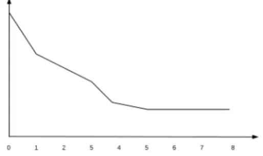
are common points between them. In Figure 1 we observe the curve of the WCET of a task ti in function of the amount of cache that it dispose of.

Figure 1: WCET depending of the number of partitions

The first common point between tasks is that there is a huge difference between C_i0 and C_i1. In the most cases the tasks will dispose of at least one cache partition. Then we call C_i1 the initial WCET of the task ti and the

initial utilization Ci1

Pi, noted U (ti).

Optimal number of partitions. Another common point is that for certain tasks which are sufficiently small, there is a WCET from which adding cache partition has no effect. We call the number of partition cor-responding to this amount of cache optimal number of partition, noted κi

defined as the following : Cκi i = min{C k i|∀k0 > k, Cik≤ Ck 0 i }

(15)

Variability. It’s important to determine if the WCET of a task varies greatly or little when allocating more cache to it. The variations of WCET can be very different depending of the nature of task. In consequence we define an approximation of the WCET variability. We call variability of a task ti, noted V (ti), the absolute value of gradient of the line between its

initial WCET and its optimal WCET. Formally : V (ti) = |

Cκi

i − Ci1

κi− 1

|

The normalized variability rank is the rank of a tasks in the task set sorted by variability, divided by the total number of tasks. Thus, a nor-malized variability rank close to 1 indicate a task part of the tasks with the lowest variability of the task set.

Task scheduling In this article we focus on non-preemptive system. Non-preemptive systems are simpler when the caches are taken into account. When a task is preempted, the new tasks can potentially evict all the cache entries of the private L1 cache and the partition of the shared L2 cache. Moreover, non-preemptive systems are actually mainly used in the industry, for example in the aerospace. Therefore, we consider that the system is non-preemptive and scheduled by NP-EDF.

The system is non-pre-emptive and scheduled by NP-EDF.

3.3 Problem formalization

The considered joint tasks and cache partitioning problem consists in as-signing each task to one core and partitioning the cache among cores, such that the resulting system is schedulable under the algorithm non-preemptive EDF.

Formally, from a task set of N tasks, M cores, and K partitions, the aim is to build a configuration valid and schedulable. A configuration is a set of M pairs (τc, kc) where τc is a set of the tasks assigned to core c and kc is

the number of partition assigned to core c. We call a configuration valid if (i) it map every task to one and only one core and (ii) the total number of partitions assigned to cores is less than or equal to K. We call a configuration schedulable if the system in which the tasks and cache are partitioned as describe by the configuration is schedulable under non-preemptive EDF. configuration schedulability In a valid configuration each task is as-signed to a core which has a fixed number of partitions. Therefore, the

(16)

WCET of each task ti is known and equal to Cik. For a core (τc, kc) the

WCET of each task ti ∈ τ is Cik = W CETi(k). When obvious from context,

we use the notation Ci instead.

A core (τ , k) is schedulable with NP-EDF iff it satisfies two condi-tions [10]: X ti∈τ Ci Pi ≤ 1 (1) ∀t_i ∈ τ, ∀L, P₁ < L < Pi: L ≥ Ci+ i−1 X j=1 bL − 1 Pj cC_j (2)

The configuration is schedulable if the taskset of each core is schedulable.

4 The algorithm

Our proposition, PDAA, Period Driven Assignment Algorithm, is an algo-rithm which aims at finding a solution to the joint tasks and cache parti-tioning problem. As previously seen with the algorithm Non pre-emptive EDF, the difference of periods between the tasks mapped on the same core is critical. Hence, PDA will assign tasks to cores depending of their period, then try to explore different configuration to minimize the total utilization, in order to find a schedulable configuration.

4.1 Rationale

4.1.1 New schedulability condition and relative weight.

From condition 1, we clearly see that our algorithm will have to deal with the total utilization of the differents cores to obtain a schedulable configuration. However, condition 2 does not make appear what kind of configuration could satisfy it.

In consequence, we will instead consider a new schedulability condition, that have been shown a necessary but not sufficient condition for condition (2) [1]: ∀t_i ∈ τ : C_i+ i−1 X j=1 Cj+ uj(Pi− Pj) < Pi (3)

(17)

The algorithm tries to build configuration which satisfy this new condi-tion. However, when the schedulability of a configuration is actually tested, the condition used are condition 1 and 2.

The important part of the equation is the term uj(P i − P j). We call this

the relative weight of the task tj for the task ti. With condition 3 we clearly

see that the aim is that for each task t, minimize the sum of the relative weights for t of the tasks with a lower period than t. We see also that the more the period of t is, the bigger this sum can be.

4.1.2 Task placement

Recall that for the computation of the sum of relative weights we consider only the tasks with a lower period. We therefore can say that a task with a big utilization have to be one the tasks which have the biggest period of the core. In this manner the big utilization of the task is counted only for the few tasks which have a bigger period.

Moreover, in order to reduce the relative weight of tasks, we want the difference between period of tasks minimized, or that the utilization is small. Then, the tasks which have the bigger difference of period with the tasks that have the bigger period of a core must have small utilization.

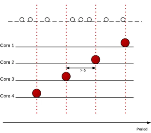
A task assignment which respect the previous directive is presented in figure 2. We’ve seen that in the returned configuration the tasks with the biggest utilization have to be the ones with the biggest period of the core.

The biggest tasks will actually be chosen having a big initial utilization and a low variability. Thus, whatever the partition among cache is, those tasks will always have a big utilization. Since condition 3 shows that two tasks with a very small difference of period have a small impact, even with a big utilization, the biggest tasks of all core are chosen in such a manner that their periods are distributed among the period interval of the taskset. Those tasks will be determinant for the placement of the other tasks. We call them critical tasks. Those tasks are represented by a big circle on the example.

As the critical tasks are considered the biggest of one core in terms of utilization, we don’t want that other tasks of greater period assigned to the core. Therefore the criticals tasks reduce the possibilities of placement of the other tasks. Thus a given task can only be assigned to a core which has a critical task of greater period than its period. On the example, each non critical task is represented by a white circle, and the period of critical task is marked with a vertical pointed line. On this example each task has to be

(18)

Figure 2: Placement of critical tasks

at the left of a critical task, therefore the possible cores are the ones with a pointed line righter than the task.

The placement which minimizes the difference of periods is when each task is assigned to the core which have the critical task with the period the closest to the task. On the example, such a placement is obtained when tasks are assigned to the lowest possible core.

However, such a placement will possibly result in cores with many tasks which will not be schedulable and cores with very few tasks. Moreover, finally, as a smaller utilization give a smaller relative pound, we want a placement which takes advantage of the optimal number of partitions and variability of task in order to optimize the cache assignment and therefore reduce the utilization of each task. More precisely, the tasks with a close optimal number of partition should be on the same core. However as it’s often not possible that all tasks have a number of partition close to the optimal, the tasks with a big variability are prioritized.

Therefore, our algorithm will ”bring up” some tasks from the unschedu-lable cores, taking account into the initial utilization and variability of the tasks as described.

4.2 The algorithm

The main steps of the algorithm are presented in algorithm 1. It takes as parameters the set τ . PDAA is divided in three main phases.

The first phase consists in obtaining the placement where all tasks are assigned to the lowest possible core.

(19)

First the critical tasks are determibed,assigned to the cores, and then removed from the tasks set. Hence φ0 is the configuration with the critical tasks assigned, and τ0the task set without the critical tasks. Thoses two sets are fixed and not modified afterward. Second the others tasks are assigned in such a way to reduce the difference of their period and the periods of already placed tasks. Then, the allocate cache min function is invoked. Algorithm 1

function PDAA φ ← ∅

(φ0, τ0_{) ← place bigger task(τ )}

φ ← place other tasks(τ0, φ0)

φ ← assign cache min(φ)

while ¬ is schedulable(φ)∧i < nbT ry do

φ ← move tasks(τ0,φ0, φ)

φ ← assign cache min(φ) i ← i + 1

end while

if is schedulable(φ) then φ ← assign total cache(φ) return φ

end if return ∅ end function

The aim of assign cache min function is to determine if there exists an assignment of cache partitions for which the configuration is schedulable. The function assigns the minimal number of cache partitions to a core for which it is schedulable. Hence the sum of minimal number of cache partition of all core might be greater than K, when there is no cache partition which allows the configuration to be schedulable and the tasks have to be moved. During the second phase different solutions are explored. While the cur-rent configuration is not schedulable, the algorithm tries to bring up some tasks taking account the variability and initial utilization. Then, the as-sign cache min is invoked again to check if there exist a schedulable config-uration. If not, tasks are moved again. The number of time this loop is executed(nbT ry) is a parameter of the algorithm, that will be discussed in section 5.

When a schedulable configuration is found, the assign total cache function assigns all the cache partitions with a greedy algorithm in such a way that the

(20)

number of partitions allocated per core is greater than its minimal number of partition.

If no schedulable congiration is found, the algorithm return ∅. Phase 1

Identification and placement of critical tasks. The first step of the algorithm is to assign the critical tasks to the cores. It’s done in the function place critical task presented in algorithm 2. The critical tasks are those which have a big initial utilization and a small variability. Thus, the tasks are sorted by utilization, and taken in decreasing order.

For each tasks, the normalized variability rank is computed.

If the normalized variability rank is bigger than a given threshold, then the tasks is considered to be part of the biggest task of the tasks set, and will be assigned to a core.

Algorithm 2

function place critical tasks(τ ) φ ← ∅

τ0_{← τ}

threshold ← 0.9

while card(φ) ≤ M ∧ treshold > 0 do

for all t ∈ τ0 by decreasing utilization do

v ← normalized variabily rank(t, τ ) if v > threshold then if ¬(∃(τ, y) ∈ φ, t0 ∈ τ ∧ |P (t) − P (t0_{)| < δ) ∧ card(φ) ≤ M then} τi= {t} τ0 ← τ0_{− {t}} φ ← φ ∪ (τi, 0) end if end if end for threshold ← threshold − 0.1 end while return (φ, τ0₎ end function

As previously said, the period of critical tasks of each core has to be far from each other. Then if the chosen tasks have a period close to a biggest task already assigned, then it assigned to this core. Else, it’s assigned to a new core. Two tasks are considered close if the difference of their period is lower than δ. This process is repeated until there is no more tasks in the

(21)

taskset. If all the cores have a critical task, then the function returns. Else, the threshold is decreased and the whole process repeted with the remaining tasks.

Once the biggest tasks are assigned the configuration is stocked in φ0. In the following of the algorithm, φ0 will never be modified. In contrary, the other tasks can be moved and a total configuration at any point of the algorithm is stored in φ.

placement of other tasks An initial placement is achieved vy func-tion by place other tasks. Since the tasks must not be assigned to a core with a critical task with a lower period than it, the possible cores for a task are determined by its period. The first placement is such that the difference beetween period is minimized . Hence each tasks is assigned to the core which have the critical tasks with the minimal period greater than its. This is the configuration in which the tasks are at the lowest possible core. Cache assignement The cache min assignment is presented in algorithm 3. This function is quite simple. For each core the function assigns a number of partitions, then test if the core is schedulable. If not, the number of partitions is increased by 1. If it is, the minimum numbers of partitions is reached. If a core is not schedulable with K partitions, then the number of partitions assigned is K + 1. Thus, if the total amount of number of partitions is lesser than K, the configuration is schedulable.

Algorithm 3

function assign cache min(φ) for all c = (τ, y) ∈ φ do

i ← 0 c ← (τ, i)

while ¬ is core schedulable(c) ∧i ≤ K + 1 do i ← i + 1 c ← (τ, i) end while end for end function phase 2

Moving Task The function Move task is presented in algorithm 4. Since the place other task function assign the task at the lowest possible

(22)

core, the move other task function will push some tasks up. With the result of allocate task min, it’s possible to know wich cores are not schedulables (those with a number of partitions greater than K).

For each unschedulables core the task that will be pushed up is chosen by the function max score task. The aim is that after the move, the total utilization of the core is highly decreased. Thus, the task chosen must have a big initial utilization. After the move, the core which will get the task must not increase its utilization too much. Since this core will be chosen in a such manner that the already assigned task will have a optimal number of partition close to the moving task, the moving task is chosen with also a big variability. The score of a task t is then αU (t) + βV (t). The task with the maximal score is chosen to be moved. α and β will be determined empirically.

Next, the set of core ”upper” than the considered core is computed by get upper core. The core chosen is the core with the minimal difference between the average optimal number of partition of assigned tasks and the optimal number of partition of the moving task.

Algorithm 4

function move task(τ0, φ)

for all c = (τc, kc) ∈ φ do

if ki= K + 1 then

C ← get upper cores(c)

t ← max score task(τi)

c0← max core affinity(C, t)

Move task(t, c, c0)

end if end for end function

phase 3 The total cache assignment tries to reduce the utilization of a schedulable configuration. At the beginning, K partitions are assigned to each cores. Then, for each core if the minimal number of partitions is not reached, the total utilization with a the number of partitions minus one is computed. the core with the biggest utilization reduction has its number of partitions assigned decrease by one. This process is repeated until K partition are assigned.

(23)

5 Experimental results

We have implemented PDAA and IA3 and compared the two algorithms on synthetic tasksets. We present in this section the performance metric for the evaluation algortihm, how the tasks are generated, the determination of empirical results of PDAA, and finally a comparison between the two algorithms.

5.1 Methodology

5.1.1 Performance metric

In order to compare the algorithms, we have to define a metric of their performance. We will use the percentage of schedulable configurations of an algorithm among the taksets generated. We then want to see the evolution of this metric in function of variations of parameters . Every experiment will report the average of 100 task sets.

5.1.2 Tasksets generation

The task set generation process consists in generating N tasks with a total utilization Usum. Usum is the sum of the worst utilization of the tasks. The

worst utilization is the utilization of the tasks without any cache available. At the end of the partitioning the total utilization is then largely lower than Usum since each task will have some cache space reserved. In consequence

we will test our algorithm with tasks with Usum> M .

Bini et al. [3] have shown that the utilization for tasks have to follow a continuous uniform law, in order that the test is not biased. They also provide an efficient algorithm to generate those utilizations. We’ll then use it to obtain the worst utilization of the tasks noted U_i0.

For a task ti we can compute the worst WCET Ci0 = Ui0× Pi. With

a coefficient c picked randomly between 0.2 and 0.4, the best WCET is Cκi

i = cCi0. The number of partitions of partition κi is picked randomly

between the lowest and the highest optimal number of partition which are part of the parameters. Finally, the others WCET of ti are determined: the

WCET for number of partition greater than the optimal number of partition are equal to Cκi

i . Other WCET are on the line ((Ci0, 0), (C κi

(24)

5.2 Determination of the parameters of PDAA

5.2.1 Choice of fixed parameter

For the evaluation of the performance of our algorithm, we’ll measure the performances in function of parameters of the input or of the systems. More precisely, the parameter of the input task set are the total utilization, the number of tasks, the lowest and the highest number of partitions. The parameter of the system that we’ll make vary is the number of cores, the amount of cache and the number of partitions. In a first time we’ll chose definitive value for some parameters, then, we’ll run experiments to deter-mine the value of the parameter of the algorithm.

Lowest and highest optimal number of partitions. Preliminary ex-periment have shown that the lowest and highest optimal number of parti-tions have no effects on the performance of the algorithms. Consequently, for the experiments presented in this section, we’ll chose for the lowest num-ber of partition the numnum-ber of partition which correspond to a size equal to

S

128 and for the highest the number which correspond to S 2.

Number of partitions. We then run different tests for a fixed load on differents numbers of cores and differents numbers of tasks. Figure 3,4 show the evolution of the efficiency of PDAA for different numbers of tasks on respectively 2 and 4 cores. Results for 6 and 8 cores are similar.

We see that under a certain number of partitions, the algorithm is not able to compute schedulable configurations. However, over a certain num-ber of partitions, increasing the numnum-ber of partitions does not increase the efficiency of the algorithm. Thus, we’ll use the value 10 for all the following experimentats.

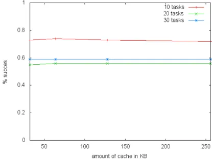
Cache size. Next, we run tests in order to determine the impact of the cache size on the percentage of the schedulable configuration returned. As presented previously, Figure 5,6 presents the results. The amount of cache make no difference here, thus we chose a typical cache size of 128KB. 5.2.2 Empirical parameters

With the parameters determined above, we want to choose value for the empirical parameters used by PDAA. Recall that we have four empirical parameters:

(25)

Figure 3: percentage succes for different numbers of partition with 2 cores

Figure 4: percentage succes for different numbers of partition with 4 cores

(26)

Figure 5: percentage succes for different cache sizes with 2 cores

Figure 6: percentage of succes for different cache sizes with 4 cores

(27)

• the number of attempts to re-allocate a task before giving up returning a schedulable configuration : nbT ry

First, we set nbT ry to a big value (2N ), so that it will no interfer with other experiment. Then, we’ll run tests to determine the other parameter. Finally, we reduce nbT ry in a such manner that a greater value value makes few difference in the performance.

Delta The parameter δ as presented previously is actually composed of a fixed part that we will not make vary. Precisely, if Pmin is the minimal

period of the input taskset and Pmax the maximal period, δ is defined such

that :

δ = Pmin− Pmax

M ×

∆ 100

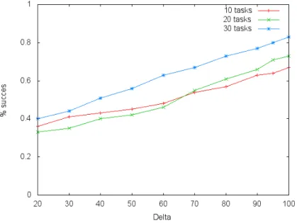
Thus, the interval of the periods of the input task set is divided by M. δ is actually ∆% of the result. What will be determined empirically is ∆.

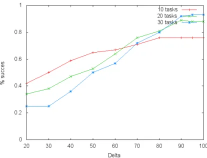
Figure 7: percentage of succes for different values of ∆ on 2 cores Figure 7, 8, 9 present the result for 2,4 and 6 cores. We see that the efficiency depends largely on this parameter. The efficiency is maximized for almost every test presented when ∆ = 90. We thus choose this value.

(28)

Figure 8: percentage of succes for different values of ∆ on 4 cores

Figure 9: percentage of succes for different values of ∆ on 6 cores

α and β Because of time constraints, there is no experiments yet for the determination of α and β. Therefore, there are arbitrarily fixed to 1. Thoses

(29)

parameters can only have influence on the choice of the tasks moved during the deplacement part of the algorithm. Therefore we can only expect few improvements with better values.

NbTry Finally, we ran the experiments with different valure of the nbT ry parameter. For the previous experiment, we had nbT ry = 2N . We tested with value N , N/2 and N/3. This made absolutly no difference in every experiment that we made, so we chose the lowest value : nbT ry = N/3.

5.3 Comparison with IA3

Finaly, we run experiment in order to determine if PDAA is more efficient than IA3 in terms of percentages of schedulable tasksets. We ran three experiments. First, for a given number of cores and a given number of tasks, we evaluate the efficiency in function of the total utilization. Then, we present experiments that describe the efficiency in function of the number of tasks. Finally, we make vary the number of core, in order to see if PDAA could take benefit of more cores in order to improve the efficiency.

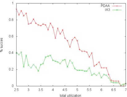
Load Figures 10, 11, 12 present the percentage of schedulable configura-tion in funcconfigura-tion of the total utilizaconfigura-tion of the taskset.

We can observe that PDAA is better than IA3, especially on system with 4 and 6 cores.

number of tasks Figures 13, 14 present the percentage of schedulable configuration in function of the number of task for a fixed total utilization. We see that the number of task has little influence of the percentage of schedulable configuration. We can notice a for both PDAA and IA3 a small improvement when the number of task is increased. We explain that by the fact that with more task for a given total utilization, tasks will trend to have smaller utilizations and then the algorithms can distribute the load among core more finely.

number of core (scalability) Finally, we test the scalability of the al-gorithm. We measured the efficiency metric in function of the number of core, for 20 tasks. Figure 15 and 16 present the result for a total utilization equal to respectively 6 and 9.

We clearly see that PDAA take benefit of more core while IA3 is non-scalable.

(30)

Figure 10: percentage of succes for differente values of total utilization on 2 cores

(31)

(32)

Figure 14: percentage of succes for different number of tasks on 6 cores

Figure 15: percentage of succes for different numbers of cores with Usum = 6

6 Conclusion and future work

(33)

Figure 16: percentage of succes for different numbers of cores with Usum = 9

in terms of our metric of efficiency. This result is obtained by taking into account the repartition of the periods of tasks of one core, which is critical in a system scheduled by NP-EDF. Moreover, PDAA is much more scalable than IA3, since it takes benefit of all core instead of trying to reduce the number of core used.

However, there are multiple possible improvements. First, we plan to extend the algorithm to work with a full cache hierarchy, not only with the L2 cache. Another possibility is to search for a preemptive algorithm. Finally, an important future work is to improve the representativity of the evaluation by experimenting on a real application and validate the task set generation.

References

[1] K. Albers and F. Slomka. An event stream driven approximation for the analysis of real-time systems. In Real-Time Systems, 2004. ECRTS 2004. Proceedings. 16th Euromicro Conference on, pages 187 – 195, june-2 july 2004.

(34)

[2] Sanjoy Baruah and Nathan Fisher. The partitioned scheduling of spo-radic real-time tasks on multiprocessor platforms.

[3] Enrico Bini and Giorgio C. Buttazzo. Measuring the perfor-mance of schedulability tests. Real-Time Systems, 30:129–154, 2005. 10.1007/s11241-005-0507-9.

[4] Bach D. Bui, Marco Caccamo, Lui Sha, and Joseph Martinez. Impact of cache partitioning on multi-tasking real time embedded systems. In Proceedings of the 2008 14th IEEE International Conference on Embed-ded and Real-Time Computing Systems and Applications, pages 101– 110, Washington, DC, USA, 2008. IEEE Computer Society.

[5] Giorgio C. Buttazzo. Hard Real-time Computing Systems: Predictable Scheduling Algorithms And Applications (Real-Time Systems Series). Springer-Verlag TELOS, Santa Clara, CA, USA, 2004.

[6] Hugues Cass, Louis Fraud, Christine Rochange, and Pascal Sainrat. Using Abstract Interpretation Techniques for Static Pointer Analysis . Computer Architecture News, 27(1):47–50, mars 1999.

[7] Robert I Davis and Alan Burns. A survey of hard real-time schedul-ing for multiprocessor systems. Journal of Soviet mathematics, 1(216682):590–669, 2010.

[8] Damien Hardy, Thomas Piquet, and Isabelle Puaut. Using bypass to tighten wcet estimates for multi-core processors with shared instruction caches. In Proceedings of the 2009 30th IEEE Real-Time Systems Sym-posium, RTSS ’09, pages 68–77, Washington, DC, USA, 2009. IEEE Computer Society.

[9] Damien Hardy and Isabelle Puaut. WCET analysis of instruction cache hierarchies. Journal of system architecture, 57(7), August 2011. [10] K. Jeffay, D.F. Stanat, and C.U. Martel. On non-preemptive scheduling

of period and sporadic tasks. In Real-Time Systems Symposium, 1991. Proceedings., Twelfth, pages 129 –139, dec 1991.

[11] Yan Li, Vivy Suhendra, Yun Liang, Tulika Mitra, and Abhik Roychoud-hury. Timing analysis of concurrent programs running on shared cache multi-cores. In Proceedings of the 2009 30th IEEE Real-Time Systems Symposium, RTSS ’09, pages 57–67, Washington, DC, USA, 2009. IEEE Computer Society.

(35)

[12] Jochen Liedtke, Hermann H¨artig, and Michael Hohmuth. Os-controlled cache predictability. In Proceedings of the 3rs IEEE Real-time Tech-nology and Applications Symposium (RTAS), Montreal, Canada, June 1997.

[13] Marco Paolieri, Eduardo Quiones, Francisco J Cazorla, Robert I Davis, and Mateo Valero. Ia3: An interference aware allocation algorithm for multicore hard real-time systems. 2011 17th IEEE RealTime and Em-bedded Technology and Applications Symposium, pages 280–290, 2011. [14] J. E. Sasinowski and J. K. Strosnider. A dynamic programming

al-gorithm for cache memory partitioning for real-time systems. IEEE Trans. Comput., 42:997–1001, August 1993.