THÈSE
En vue de l’obtention duDOCTORAT DE L’UNIVERSITÉ DE
TOULOUSE
Délivré par: Université Toulouse III – Paul Sabatier
École doctorale: Mathématiques Informatique Télécommunications (MITT) Unité de recherche: UMR 5219
Discipline : Mathématiques
présentée par
Arnaud MORTIER
Nouveaux aspects combinatoires de théorie des nœuds
et des nœuds virtuels
dirigée par Thomas FIEDLER
Soutenue le 12 juillet 2013 devant le jury composé de :
M. Christian Blanchet
Paris VII
examinateur
M. Thomas Fiedler
Toulouse III
directeur
M. Louis Funar
Institut Fourier rapporteur
M. Gregor Masbaum
Paris VI
examinateur
M. Jean-Baptiste Meilhan Institut Fourier examinateur
M. Michael Polyak
Technion
rapporteur
Remerciements
Avant tout je présente mes excuses aux personnes qui m’ont accompagné ou soutenu durant les quatre dernières années, pour le grand nombre de formalités et d’euphé- mismes contenus dans ces remerciements. Il peut être très difficile de ré-sumer en quelques mots la reconnaissance accumulée au cours d’une période aussi longue. Tout comme il est difficile de ne pas donner à de tels propos une allure d’épilogue.
Je remercie Thomas Fiedler. Pour la confiance qu’il n’a cessé d’avoir en moi, depuis le début et à travers des périodes très incertaines. Pour la souplesse et l’autonomie qu’il m’a laissées, sans être jamais à court de ressources, d’idées, de références, de contacts, lorsque le besoin pouvait s’en faire sentir. Pour être, enfin, l’instigateur d’une école d’hiver d’une richesse mathématique et humaine que je ne saurais décrire par des mots.
I wish to thank Misha Polyak. Because he accepted the task of being a referee to this thesis report. For the uninterrupted flow of his ideas merging topology, algebra and combinatorics, which were a great source of inspiration over the past years. For being, in some sense, my virtual co-advisor.
Je remercie Louis Funar et Gregor Masbaum pour avoir accepté de faire partie de mon jury, et Louis en particulier pour m’avoir donné son temps en relisant ce manuscrit.
À Jean-Baptiste Meilhan, je souhaiterais dire merci pour s’être intéressé à mon travail – et avoir sincèrement proposé d’être rapporteur de cette thèse, avant qu’une subtilité bureaucratique ne l’en empêche. Pour m’avoir invité à Grenoble, et permis de participer aux événements organisés dans le cadre de l’ANR VasKho.
Pour n’oublier aucun membre du jury, je souhaite exprimer ma profonde recon-naissance à Christian Blanchet, pour n’avoir jamais refusé une conversation, pour ses conseils (méta-)mathématiques et son soutien – qui m’a notamment permis de passer une année extrêmement enrichissante à Paris.
I would like to thank a number of people who accepted to share their ideas with me, namely Fionntan Roukema and Micah Chrisman with whom I had interesting conversations over the internet, and Matthew Hedden, Jean-François Barraud and Benjamin Audoux who are responsible for the little I know about Heegaard-Floer homology.
Je tiens à remercier Ana Lecuona, Hoel Queffelec et Catherine Gille pour une col-laboration inoubliable, qui m’a fait découvrir à quel point il peut être non seulement agréable, mais aussi productif, de travailler en groupe.
De trois ans passés à Toulouse, je garderai le souvenir de Michel Boileau et Joseph Tapia, qui ont une tendance innée à négliger leurs intérêts personnels pour prêter une attention sincère au néophyte et tenter de lui transmettre leurs connaissances, ne fût-il capable d’en absorber qu’une quantité finie.
Je me souviendrai de Jacques Sauloy, Claire Dartyge, Philippe Monnier, Ahmed Zeriahi et Anne Cumenge avec qui ce fut un plaisir d’enseigner – plaisir qui a pu se révéler réciproque, notamment lorsque Jacques a amicalement tenté de me dissuader de déménager à Paris.
Un grand merci à mes coburettes Virginie, Claire et Valentina (par ordre alphabé-tique des noms de famille, comme c’est d’usage en mathémaalphabé-tiques lorsqu’aucun autre ordre ne s’avère plus naturel), pour le café, les kalanchoes, la chauffeuse à sieste, la scopa, les dessins millénaires au tableau, la bonne humeur (meur, meur, meur-meur) qui a régné dans le bureau 105 pendant ces années, ponctuées par les passages éclair de Dima que je remercie pour les cours de russe et les cours de durak.
Merci à JC et Marie-Anne pour leur amitié, les soirées, le festival du cinéma d’Amérique latine, la coinche... Merci à Sébastien, Paul et Daniel pour les parties d’échecs, à Arnaud et Pascale pour les bons moments passés autour d’un pique-nique ou d’un barbecue. Merci à Gioia pour si bien porter son prénom.
Avant de continuer, le lecteur doit réaliser que la période de fin d’études doc-torales est assez éprouvante. Surtout les 36 derniers mois, dirait Coluche. Afin de tenir psychologiquement, il est de bon aloi de réserver une place incompressible à l’humour et à l’invraisemblable. Je ne peux que respecter cet état d’esprit en remer-ciant les personnes qui m’ont accompagné durant cette période et notamment les occupants des bureaux 7C08 puis 750, qui étaient pour beaucoup dans une situation similaire, et sans lesquelles la survie n’aurait pas été acquise.
Merci à LH et Lukas pour d’enrichissantes conversations, notamment sur les 3-coloriages de graphes bipartites, et sur les meilleures proportions thé/café dans lesquelles il convient d’arroser un cactus à raquettes. À Hoel pour sa preuve élégante de la primalité de 2013 (ainsi que d’autres nombres dont les mathématiciens ont longtemps mis en doute le caractère premier en raison de leur divisibilité par 2). À Elodie, pour ses connaissances en labyrinthes administratifs, pour la logistique pain/nutella/sopalin des pauses café, et pour les regards noirs qu’elle m’a valus en envoyant des e-mails calomnieux à ma femme. À Roro, le Chinois du Cambodge qui sait parler aux filles (en langage des singes), pour avoir porté mes slips (afin de donner un coup de main lors de mon déménagement à Paris), pour les week-ends studieux à Sophie Germain, et enfin pour m’avoir promis une côte de bœuf pour figurer dans ces remerciements. À Christophe, pour ses macarons ratés, pour les pauses chocolat aux horaires très stricts, pour croire sérieusement que des gens s’enferment dans les bureaux de Sophie Germain pour y développer des photos. À Xin, Sary et Alexandre, pour avoir préservé une part de sagesse dans le quotidien des doctorants.
Une pensée particulière à destination de Pascal Chiettini, secrétaire dont l’efficaci-té comme la disponibilil’efficaci-té ne semblent pas avoir de limites.
Enfin, merci à ma famille, mes parents, Vika, pour me supporter, pour croire en moi, pour me garder dans le droit chemin. Vika, sans toi ce manuscrit ne serait pas. Je te dois un café.
Contents
1 Introduction 7
1.1 Conventions . . . 11
2 Virtual knot theories 13 2.1 The classical case . . . 13
2.1.1 “Real” knots in S3 and their Gauss diagrams . . . 13
2.1.2 The birth of virtual knot theory . . . 17
2.2 Knot diagrams on an arbitrary surface . . . 18
2.2.1 Thickened surfaces . . . 18
2.2.2 Diagram isotopies and detour moves . . . 21
2.3 Virtual knot theory on a weighted group . . . 22
2.3.1 General settings and the main theorem . . . 22
2.3.2 Abelian Gauss diagrams . . . 28
2.3.3 Homological formulas . . . 32
3 Arrow diagram formulas for virtual knots 39 3.1 Finite-type invariants . . . 40
3.2 Gauss diagram invariants . . . 42
3.2.1 General algebraic settings . . . 42
3.2.2 The symmetry-preserving injections . . . 46
3.2.3 Arrow diagrams and homogeneous invariants . . . 49
3.3 Polyak’s conjecture . . . 55
3.3.1 Based and degenerate diagrams . . . 56
3.3.2 Detecting arrow diagram formulas . . . 57
3.3.3 Invariance criterion for w-orbits . . . 60
3.3.4 The topological viewpoint . . . 63
3.4 Examples and applications . . . 69
3.4.1 Grishanov-Vassiliev’s planar chain invariants . . . 69
3.4.2 There is a Whitney index for non nullhomotopic virtual knots 71 3.4.3 Some more computations . . . 74
4 Towards detection of closed braids 77 4.1 Tangles and T-diagrams . . . 77
4.1.1 T-diagrams of real knots . . . 79
4.2 A characterization of closed braid diagrams . . . 83
4.2.1 Positive admissible T-diagrams are represented by braids . . . 84
4.2.2 Admissible implies positive . . . 86 5
4.2.3 Asymptotic admissibility . . . 89
4.3 How to take care of Reidemeister moves – a conjecture . . . 91
4.3.1 Trace graphs . . . 92
4.3.2 A normal form for trace graphs . . . 94
4.3.3 Some ideas that do not work (yet) . . . 98
5 Invariants of non generic homotopies 103 5.1 Triple homotopies . . . 104
5.2 A non trivial triple loop . . . 106
Chapter 1
Introduction
Gauss diagrams
A Gauss diagram is the result of unknotting a knot diagram in the plane, using arrows to remember which couples of points of the circle were originally crossed. To make the construction faithful – that is, with no essential loss of information –, one also remembers the over/under datum and the local writhes of the crossings.
One observes that not all Gauss diagrams actually come from knots. By forget-ting the 3-space and the actual knots, considering only Gauss diagrams and their combinatorics (also made of “Reidemeister moves”), one obtains the virtual knot
the-ory, developed by Kauffman [17] in the late 90’s. It happens that virtual knots can
also be understood in terms of knot diagrams in the plane, with usual and virtual crossings, subject to usual, virtual and mixed Reidemeister moves. These last two additional kinds of moves are precisely those leaving the underlying Gauss diagram unchanged. Together, they are equivalent to the single detour move, which is global – one or the other viewpoint can be more convenient depending on the situation. An important result of Kauffman [17] states that the additional virtual moves cannot connect different usual knot types.
Knot theory in R3
Knot diagrams in R2 Reidemeister moves
Classical Gauss diagrams
R-moves
≃ Virtual knot diagrams in R2
Reidemeister moves + detour move
projection
In Chapter 2, we aim at generalizing this scheme following the initial idea of replacing the projection R3 → R2 with a real line bundle over an arbitrary surface Σ – which is called a thickened surface.
To circumvent algebraic issues about conjugacy in free groups, the knots con-sidered have all of their usual crossings lying over a fixed contractible subset of Σ. Also, every usual Reidemeister move can be made to happen over that set by an adequate diagram isotopy. This splits the tasks into two parts: understanding the
local Reidemeister moves (which are nothing more than what one is used to), and
understanding the global diagram isotopies and detour moves. It is shown that these global moves are essentially generated by the elementary move taking a real crossing and moving it all along a given loop in Σ.
From the Gauss diagram viewpoint – assuming for now that Σ is orientable:
➺ Gathering all the real crossings over a disc allows one to color the edges (the parts of the circle between two consecutive arrow ends) with elements of
π= π1(Σ).
➺ The Reidemeister moves are the same as usual, with the requirement that the edges involved must be marked the unit 1 ∈ π.
➺ As before, the detour moves do not change the diagram at all.
➺ There is a new conjugacy move corresponding to an elementary global move. It changes the π-markings of the four edges adjacent to an arrow.
The case of non orientable surfaces requires only little more effort: some of the Gauss diagram decorations may not be globally defined, in which case the conjugacy move can change them too, according to their monodromy. When the total space of the bundle is assumed to be orientable, then there is only one monodromy morphism to consider, and it is given by the first Stiefel-Whitney class of the tangent bundle to Σ.
With all this in mind we define a new Gauss diagram theory, that depends only on an arbitrary group π and a homomorphism w : π → F2 (Section 2.3). Just like the usual virtual knot theory gives up caring about the actual existence of knots, this “virtual knot theory on a group” ignores the existence of a surface on which to draw diagrams. As expected, for an arbitrary surface Σ, the input π = π1(Σ) and w ≡ w1(T Σ) (the first Stiefel-Whitney class) gives a theory that fully and faithfully encodes virtual knot diagrams on Σ up to Reidemeister moves, diagram isotopy and detour moves. It follows that when two surfaces happen to thicken into the same 3-manifold M – such as the annulus and the Moebius strip, one obtains different
“virtual” generalizations of knot theory in M. However, when π1(M) 6= {1}, it is not known whether the usual knot theory in M faithfully embeds into any of these virtual generalizations.
Knot theory in the thickening of Σ
Knot diagrams in Σ
Reidemeister moves
Gauss diagrams on π1(Σ) R-moves and conjugacy moves
≃ (Theorem 2.3.3) Virtual knot diagrams in Σ
Reidemeister moves + detour move
bundle projection
A slightly more compact version is defined when the group π is abelian, inspired by T.Fiedler’s diagrams decorated with elements of H1(Σ) [10, 9]. It allows one to get rid of the conjugacy moves, with no loss of information. In general, a description of the orbits of the conjugacy moves by diagrams with finitely many decorations is not known. It is related to the existence of an algorithm to decide whether two given Gauss diagrams are related by conjugacy moves. We discuss that question in Subsection 2.3.1 – paragraph About the orbits of w-moves.
Finite type invariants
Besides the encoding of knot diagrams, a major feature of Gauss diagrams is that they provide a combinatorial description of Vassiliev’s finite type invariants. This so called theory of Gauss diagram formulas was developed by M.Polyak and O.Viro [27], and independently by T.Fiedler [9]. A few formulas due to J.Lannes [19] for the invariants up to degree three do the same computations and came up simultaneously, though without the powerful diagrammatic aspect. All of these invariants are of finite type in the sense of Vassiliev. An important theorem of M.Goussarov [13] states that conversely, in the classical case of knots in R3, every Vassiliev invariant happens as a Gauss diagram formula.
Roughly, a Gauss diagram formula computes a weighted sum of the subdiagrams of its variable. An important particular case is that of arrow diagram formulas, whose weights satisfy the following rule: if two diagrams differ only by the signs of
their arrows, then either their weights are 0, or the ratio of their weights is equal to the ratio of the products of their signs. Historically, this particular case was the first
to appear (see [27]). Most examples still belong in this case at the time of writing (see [3], [4], [15]).
One observes that these invariants are naturally defined, as maps, on the set of all Gauss diagrams. It raises the question: which of them do also define invariants of virtual knots? This question is investigated in [14], where it is shown that the Q-space of virtual Gauss diagram formulas identifies with the dual of the Polyak
algebra from [25]. Also in [14], an alternative notion of finite-type is developed,
axiomatizing those virtual knot invariants that come from Gauss diagram formulas. Besides this virtual direction, a number of generalizations of Gauss diagram formulas have been made for knot diagrams in a surface Σ, using different kinds of
additional decorations – for instance free homotopy classes of loops in Σ [15], and elements of quotients of H1(Σ) [10]. All of these frameworks are “contained” the above Gauss diagram theory on a group.
Chapter 3 is devoted to the study of the virtual invariants in the framework of Gauss diagrams on a group. It generalizes [22] where only the case of knot diagrams in R × S1 was considered.
We formalize the fact that it should contain the existing theories by describing appropriate “symmetry preserving” maps: a space with few information and lots of symmetries injects into a space with more information and less symmetries.
A Polyak algebra is constructed. It allows one to observe numerous relations between arrow diagram formulas and homogeneous Gauss diagram formulas, which finally lead to show that these two notions coincide (Theorem 3.2.24). Special invariance criteria follow for arrow diagram formulas. In particular, the Reidemeister III criterion (Theorem 3.3.9) gives an interpretation and a proof of a conjecture of M.Polyak, which predicts that arrow diagram formulas should be the kernel of a map with values in some space of degenerate diagrams. Subsection 3.3.4 contains a topological point of view on this map, at the intersection between M.Polyak and V.A.Vassiliev’s ideas. This point of view is the most likely to give rise to a full cohomology theory, in which the above map would be the 0-coboundary.
Once the invariance criteria have been described at the top-level (that of arrow diagrams on a group), thanks to the symmetry-preserving injections one directly obtains criteria for all the kinds of invariants that lie “below”. Chapter 3 ends with examples that take advantage of this fact. In particular, we give an alternative proof to Grishanov-Vassiliev’s theorem on planar arrow diagram formulas [15] and slightly improve it.
Detection of closed braids in the solid torus
The closed braid problem is the following: given a knot diagram in the annulus R × S1, how to tell if it represents a knot that is isotopic to a closed braid in the solid torus [16]?
In [10], T.Fiedler suggests an attempt to answer that question by evaluating specific finite-type invariants, which conjecturally all vanish if and only if the knot is a closed braid. Only a few examples are constructed. The reason why the invariants from these examples vanish on closed braids is that they weight only diagrams that cannot happen as subdiagrams of a closed braid, because of the homology class of certain loops: those that run positively along the edges of the Gauss diagram (the
ER loops).
Chapter 4 is a draft attempt to answer the closed braid problem by a direct study of the set of these loops.
A new kind of Gauss diagrams is introduced, no more decorated by elements of a group, but by words in a fixed presentation of that group. The difference is significant – and similar to the step between Gauss diagrams with π1 decorations and those with only some h1 decorations: the more information there is in the Gauss diagrams, the more accurate will be their topological matches.
char-acterized by the fact that all ER loops must have a positive homology class in Z ≃ H1(R × S1) – a property called braid-admissibility already in [10]. We conjec-ture that for diagrams with minimal number of crossings, not being in a closed braid position implies not being equivalent to a closed braid diagram modulo Reidemeister moves. A few aspects and possible plans towards that conjecture are discussed at the end of the chapter.
Invariants of non generic homotopies
V.A.Vassiliev introduced the finite-type knot invariants by studying the topology of the infinite dimensional stratified space of all smooth immersions of a circle in R3. To define these invariants, one considers only those strata of the discriminant that correspond to singular knots with a finite number of ordinary double points.
In Chapter 5, we investigate what can happen if one avoids these strata and instead consider those with ordinary triple points. M.Heusener has proved that any knot can be unknotted by a homotopy that meets the discriminant only in such strata, even if one only allows some directions in which to cross these strata, called
coherent – that is, when on both sides of the singularity, the three crossings of the
knot diagram have the same local writhe.
By adding up all the writhe increases encountered at triple points during such a homotopy, one obtains an invariant of triple homotopies (in a sense that is made precise by defining homotopies of triple homotopies), that is shown to be non-trivial.
We show that a twisted (or weighted) form of the above invariant gives a formula for the “derivative” of the Casson invariant for knots, with respect to coherent triple points. A number of (unanswered) questions arise from there: is it possible to define a complete finite-type theory with respect to coherent triple points? How is it related to Vassiliev’s finite-type invariant theory?
1.1 Conventions
Pictures with incomplete diagrams
When several incomplete diagrams are represented side by side in a picture, or in one and the same equation, it is to be understood that
1. Every unseen part – including missing decorations, such as local orientations – is the same for all diagrams.
2. The picture is valid no matter what are those unseen parts, unless otherwise specified in the caption under the picture.
“Real” objects
The word “real” will be used to label a usual crossing in a knot diagram, or a knot diagram that only contains usual crossings, or a Gauss diagram that is represented by such a knot diagram. This terminology is justified by two reasons. First, the contrast with the word “virtual”, that labels the second kind of crossings encountered
in Gauss diagram theory. Second, a real crossing, in a diagram drawn on a surface Σ, is a double point of an immersion whose two smooth branches have been locally pushed inside a real line bundle over Σ.
I deeply apologize to the reader who is familiar with another terminology.
Notations
A notation that is absent from this list is usually specific to a section. D: a knot diagram.
G: a Gauss diagram or an abelian Gauss diagram. K: a knot, or the circle of a Gauss diagram.
R-I, R-II, R-III: Reidemeister moves of knot diagrams.
R1, R2, R3: R-moves of Gauss diagrams – matching the Reidemeister moves. ν: a knot invariant.
G: a linear combination of Gauss diagrams.
Gn: the Q-space freely generated by degree n Gauss diagrams. G≤n: the direct sum of all Gk’s for k ≤ n.
G: the direct limit of the G≤n’s with the natural inclusions.
G•: similar to G, where the Gauss diagrams have a preferred edge (Defini-tion 3.3.1).
DG: similar to G, with degenerate diagrams (Definition 3.3.1).
b
G: the Q-space of formal series of Gauss diagrams. There are similar notations for arrow diagrams:
A, A, An, A≤n, A, A•, DA, Ab. π: an arbitrary group.
h1(π): the set of conjugacy classes in π. g: an arbitrary element of π.
w: an arbitrary “weight” homomorphism π → F2. w0: the trivial homomorphism π → F2.
Σ: an arbitrary surface.
h1(Σ): the set of free homotopy classes of loops in Σ. M: the total space of an oriented real line bundle over Σ.
When a surface Σ is considered, π is set to π1(Σ) and w is set to the first Stiefel-Whitney class of T Σ. This couple is called the weighted fundamental group of Σ.
µ: the decorating map H1(G) → π of an abelian Gauss diagram G. γ: a loop S1 → G, or a homology class in H
1(G). A: an arrow of G.
e: an edge of G.
Chapter 2
Virtual knot theories
This chapter begins with a brief introduction to the classical settings of virtual knot theory via Gauss diagrams. The goal is to define Gauss diagrams in a large framework that contains virtual knot diagrams on an arbitrary surface.
Section 2.2 defines and studies (virtual) knot diagrams on an arbitrary surface Σ: these are tetravalent graphs embedded in Σ, some of whose double points (the “real” ones) are pushed and desingularized into a real line bundle over Σ. Defining Gauss diagrams requires a global notion for the branches at a real crossing to be one “over” the other, and a global notion of writhe of a crossing. It is shown that these notions can be defined simultaneously if and only if Σ is orientable. If it is not, we sacrifice the globality of one property, and take into account its monodromy. It is shown that when the total space of the bundle is orientable, the writhes are globally defined and the monodromy of the “over/under” datum is the first Stiefel-Whitney class of the tangent bundle to Σ, w1(Σ).
In Section 2.3 is given a definition of Gauss diagrams decorated by elements of a fixed group π, subject to usual Reidemeister moves, and to additional “conjugacy moves”, depending on a fixed group homomorphism w : π → F2. It is shown that when there is a surface Σ such that π = π(Σ) and w1 = w1(Σ), then there is a 1 − 1 correspondence between Gauss diagrams and virtual knot diagrams, that induces a correspondence between the equivalence classes (virtual knot types) on both sides.
A lighter kind of Gauss diagrams, called abelian, is defined in Subsection 2.3.2 following the idea of T.Fiedler’s H1(Σ)-decorated diagrams ([9]) and shown to be equivalent to the above when π is abelian and w is trivial. The little drawback of this version is that it becomes more difficult to compute the homological decoration of an arbitrary loop. Two formulas are presented in 2.3.3 to sort this out, involving quite unexpected combinatorial tools.
2.1 The classical case
2.1.1 “Real” knots in S
3and their Gauss diagrams
In the classical sense, a knot denotes a smooth embedding of a circle, which is here always assumed to be oriented, into the 3-dimensional sphere. Knots are usually considered up to isotopy: a knot type is the orbit of a knot under the action
of Diff+(S3), the group of positive (i.e. orientation preserving) diffeomorphisms of S3.
A significant part of knot theory goes through the study of knot diagrams, which are generic projections of knots on a plane (or a 2-dimensional sphere), whose double points are decorated with the datum of which branch is “over” the other. Such projections enable one to treat knots, and even knot types, as combinatorial objects: the isotopy equivalence relation, rather difficult to handle as such, splits into simple parts:
➺ On the one hand, diagram isotopy – that is, the action of positive diffeomor-phisms of the plane.
➺ On the other hand, the so-called Reidemeister moves, which actually change the underlying tetravalent graph.
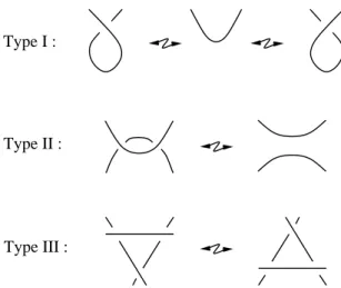
Reidemeister moves are depicted on Fig.2.1.
Type I :
Type II :
Type III :
Figure 2.1: The three types of Reidemeister moves for knot diagrams
The theory of Gauss diagrams gets rid of the “diagram isotopy” part, to keep only the combinatorial skeleton.
Definition 2.1.1. A classical Gauss diagram is an equivalence class of an oriented
circle in which a finite number of couples of points are linked by an abstract oriented arrow with a sign decoration, up to positive homeomorphism of the circle. A Gauss diagram with n arrows is said to be of degree n.
From a classical knot diagram D in R2, one obtains the associated Gauss dia-gram by considering a parametrization of D by an oriented circle, and connecting
the preimages of each crossing by an arrow oriented from the underpassing to the overpassing point (the direction of the light from the picture to the eye), given as a sign the local writhe of the crossing (see Fig.2.2).
It will often happen that we regard Gauss diagrams as topological objects (draw-ing loops on them, consider(draw-ing their first homology). In that case, one must beware of the fact that the arrows do not topologically intersect – that is what is meant by “abstract”. However, the fact that two arrows may look like they intersect is something combinatorially well-defined, and interesting for many purposes.
a
c
d
a
a
b
b
c
c
d
d
b
−
+
−
+
+
−
Figure 2.2: The writhe convention, a diagram of the figure eight knot, and its Gauss diagram – the letters are here only for the sake of clarity.
Definition-Lemma 2.1.2. Two knot diagrams in the plane with the same Gauss
diagram are isotopic to each other. In this regard, classical Gauss diagram theory is said to be faithful to real knot theory in S3.
A loop in a Gauss diagram is a continuous map S1 → G. Such a map is always homotopic to a locally injective one, so we will always assume loops to be locally injective: it is a helpful assumption to define combinatorial devices and properties. For instance, it makes sense to say that such a loop turns left at an arrow. Fig.2.3 shows 3 examples out of 8 possible local configurations.
+ + −
Figure 2.3: Paths turning left in a Gauss diagram and their knot diagrammatic version
In a knot diagram, it is possible to make two arcs cross each other by a Reide-meister II move if and only if these arcs face each other. Equivalently, there must be a path in the diagram that joins the two arcs and turns left at every crossing that it meets. Thus, one sees that Reidemeister II creating moves make sense in terms of Gauss diagrams.
In general, Gauss diagrams naturally enjoy a full set of Reidemeister moves. Fig.2.4 shows them without writhes, and Lemma 2.1.4 completes the picture.
Definition 2.1.3. In a classical Gauss diagram of degree n, the complementary of
the arrows is made of 2n oriented components. These are called the edges of the diagram. In a diagram with no arrow, we still call the whole circle an edge.
do not belong to the same arrow. Put
η(e) =
(
+1 if the arrows that bound e cross each other
−1 otherwise ,
and let ↑(e) be the number of arrowheads at the boundary of e. Then define
ε(e) = η(e) · (−1)↑(e).
Finally, define the writhe w(e) as the product of the writhes of the two arrows at the boundary of e. 1 R R 2 R 3 = = = = =
Figure 2.4: R-moves for Gauss diagrams (see Lemma 2.1.4 for the rules for the decorations)
Definition-Lemma 2.1.4. Let D be a knot diagram with Gauss diagram G, such
that G features a situation like on one of the pictures from Fig. 2.4 (say from table
Ri, 1 ≤ i ≤ 3). Then, the arcs/crossings of D corresponding to the edges/arrows of the local picture are in a position to perform a Reidemeister move of type i if and only if:
➺ i= 1. No additional condition.
➺ i= 2. The two arrows head to the same edge, and have opposite writhes, and
there is a simple path joining the two visible edges, turning left at every arrow that it meets.
➺ i= 3. The value of w(e)ε(e) is the same for all three visible edges e, and the
values of ↑(e) are pairwise different.
A picture from Fig. 2.4 is called an R-move of real Gauss diagrams as soon as it satisfies the above condition.
Remark 2.1.5. The strange sign ε will show up again, not only in other kinds of
000 111 000111 000111 000111 0 0 1 1 00 11 00 11 00 11 0 0 0 0 0 0 0 0 0 0 0 0 0 0 0 0 0 0 0 0 0 0 0 0 1 1 1 1 1 1 1 1 1 1 1 1 1 1 1 1 1 1 1 1 1 1 1 1 0000 1111 0000 1111 000 111 0 0 0 1 1 1 000 111 0 0 0 1 1 1 00 00 00 11 11 11 0 0 1 1 000 111 P P P a) b)
or
+
+
P?
P?
c)Figure 2.5: This one cannot come from a knot
2.1.2 The birth of virtual knot theory
Now a natural question is: “Is any classical Gauss diagram associated to some knot?”, and the answer is no. The simplest example is pictured on Fig.2.5: try to draw a corresponding knot diagram, you will soon find it necessary to add a crossing where no arrow allows it.
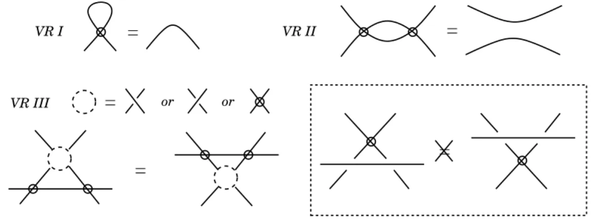
This is how virtual knot theory begins: add whichever crossings you need to complete the picture, and draw a circle around them, to notify that these are not regular crossings. These so-called virtual crossings are subject to a new set of Reide-meister moves, precisely those that leave the underlying Gauss diagram unchanged (in particular, the last move depicted on Fig.2.6 is forbidden!).
=
or or=
VR III=
=
=
VR II VR IFigure 2.6: Virtual Reidemeister moves
Definition 2.1.6. A detour move is a boundary-fixing homotopy of an arc that
goes through only virtual crossings. The arc may go across real crossings during the homotopy, and at the end it shall still contain only virtual crossings.
Fact. The full set of virtual Reidemeister moves (Fig.2.6) is equivalent to the detour
move.
Finally, we see that virtual crossings are what they were meant to be: an artefact that enables knot-diagrammatic representations of (all) Gauss diagrams, with no gain or loss of information, as formalized below:
Definition-Lemma 2.1.7. A classical Gauss diagram defines a unique virtual knot
diagram in the plane, up to diagram isotopy and virtual Reidemeister moves (or detour moves). We say that classical Gauss diagram theory is fully faithful to virtual knot theory in the plane.
Let us proceed to describing R-moves, with a virtual version of Lemma 2.1.4:
Definition-Lemma 2.1.8. Let (D, G) be a couple like in Lemma 2.1.4 – though D
is no more supposed to be real, and fix some edges/arrows of G matching a situation from Fig.2.4. Then, up to detour moves, the corresponding arcs/crossings of D are in a position to perform a classical Reidemeister move under the same necessary and sufficient conditions as in Lemma 2.1.4, except for Reidemeister II for which the “simple path condition” disappears.
Again a picture from Fig. 2.4 is called an R-move of Gauss diagrams if it satisfies the corresponding conditions.
The two previous lemmas allow one to regard virtual knot theory as the theory of Gauss diagrams, up to R-moves, completely forgetting about actual knots.
Let us end this section by mentioning a theorem due to Kauffman, which defi-nitely makes virtual knot theory satisfactory, because it really contains the classical theory:
Theorem 2.1.9 (Kauffman [17], see also [14]). Any two knots in S3 with diagrams that may be linked by a sequence of real and virtual Reidemeister moves are isotopic.
2.2 Knot diagrams on an arbitrary surface
One goal of this chapter is to examine when and how one can define a couple of equivalent theories “virtual knots − Gauss diagrams” that generalizes knot theory in an arbitrary 3-manifold M. What first appears is that a Gauss diagram depends on a projection; so it seems unavoidable to ask for the existence of a surface Σ (maybe with boundary, non orientable, or non compact), and a “nice” map p : M → Σ. For the over and under branches at a crossing to be well-defined at least locally, the fibers of p need to be equipped with a total order: this leaves only the possiblity of a real line bundle.
2.2.1 Thickened surfaces
Let us now split the discussion according to the two kinds of decorations that one would expect to find on a Gauss diagram: signs (local writhes), and orientation of the arrows.
Local writhes
For a knot in an arbitrary real line bundle, there are situations in which it is possible to switch over and under in a crossing by a mere diagram isotopy. For instance, in the non-trivial line bundle over the annulus S1 × R, a full rotation of
P
P
P
P
Figure 2.7: Non trivial line bundle over the annulus – as one reads from top to bottom, the knot moves towards the right of the picture.
the closure of the two-stranded elementary braid σ1 turns it into the closure of σ−11 (Fig. 2.7).
Fig. 2.7 would be exactly the same (except for the gluing indications) if one considered the trivial line bundle over the Moebius strip. Note that this diagram would then represent a 2-component link. In fact, it is possible to embed this picture in any non-orientable total space of a line bundle over a surface.
This phenomenon reveals the fact that in these cases, there is no way to define the local writhe of a crossing.
Definition 2.2.1. We call a thickened surface a real line bundle over a surface,
whose total space is orientable.
Definition-Lemma 2.2.2. If M → Σ is a thickened surface, then its first
Stiefel-Whitney class coincides with that of the tangent bundle to Σ. This class induces a homomorphism w1(Σ) : π1(Σ) → F2. The couple (π1(Σ), w1(Σ)) is called the weighted fundamental group of Σ. Note that in particular the thickening of Σ is the trivial bundle Σ × R if and only if Σ is orientable.
There is a general definition of the writhe in these settings – see [7], Lemma 1. Let us repeat it for the sake of completeness.
Let K : S1 → M be an oriented knot in an oriented thickened surface M → Σ, in generic position with respect to the bundle projection. Pick a double point p of the projection (i.e. a crossing), and choose an orientation of the fibre Mp. This
orientation induces a total order on Mp, and defines an over branch and an under
branch. By genericity, these may not be tangent through the projection, so the triple (under, over, fibre) defines an orientation on M.
Definition-Lemma 2.2.3. The writhe of the crossing at p is set to +1 if the
orien-tation defined above coincides with the fixed orienorien-tation of M, and −1 if not. This does not depend on the choice of an orientation of Mp.
Remark 2.2.4. It appears that the writhe of a crossing depends on a choice, that of
an orientation for M. The important thing is that this choice is global, so that it makes sense to compare the writhes of different crossings (they live in “the same” Z/2Z).
Arrow orientations
In the classical case, the orientations of the arrows in the Gauss diagram of a knot were defined according to which branch of each crossing was over the other. This assumed the choice of a position for the eye looking at the diagram, more formally an orientation for each fibre of the bundle.
For a knot in a general thickened surface, one can still orient the fibres over little neighborhoods of the crossings, thus defining an orientation for each arrow. But the fact of representing each all of these data with the same binary decoration, without any more information, implies that they can be compared – that they rely on a global definition (see Remark 2.2.4). This is possible only if the bundle is trivial, which, according to our definition of a thickened surface, happens only if the surface is orientable.
So it seems that one has a choice to make, either restricting one’s attention to orientable surfaces, or taking into account the monodromy of whatever is not glob-ally defined. Additional conjugacy moves will be needed when one defines Gauss diagrams – see section 2.3. The convention to consider only fibre bundles with an orientable total space is arbitrary, its only use is to reduce the number of monodromy morphisms to 1 instead of 2.
Fix an arbitrary surface Σ and denote its thickening by M → Σ.
Definition 2.2.5. A virtual knot diagram on Σ is a generic immersion S1 → Σ whose every double point has been decorated
➺ either with the designation “virtual” (which is nothing but a name), ➺ or with a way to desingularize it locally into M, up to local isotopy.
These diagrams are subject to the usual Reidemeister moves depicted on Fig.2.1, and to detour moves (Definition 2.1.6), which are still equivalent to the set of virtual Reidemeister moves from Fig.2.6.
➺ If one chooses an orientation for M, then the real crossings of a virtual knot diagram have a well-defined writhe.
➺ There is no way to associate a classical Gauss diagram with such a knot, unless Σ is orientable.
2.2.2 Diagram isotopies and detour moves
Here by knot diagram we mean a virtual knot diagram on a fixed arbitrary surface Σ, as defined above. In this case a diagram isotopy, usually briefly denoted by H : Id → h, is the datum of a diffeomorphism h of Σ together with an isotopy from IdΣ to h. A detour move is a boundary-fixing homotopy of an arc that, before and after the homotopy, goes through only virtual crossings (such an arc is called
totally virtual). Though both of these processes seem rather simple, it will be useful
to understand how they interact.
Lemma 2.2.6. A knot diagram obtained from another by a sequence of diagram
isotopies alternating with detour moves may always be obtained by a single diagram isotopy followed by detour moves.
Proof. It is enough to show that a detour move d followed by a diagram isotopy
Id → h may be replaced with a diagram isotopy followed by a detour move (without changing the initial and final diagrams). The initial diagram is denoted by D.
Call α the totally virtual arc that is moved by the detour move. By definition,
d(α) is boundary-fixing homotopic to α, and is totally virtual too. Thus, h (d (α))
and h(α) are totally virtual and boundary-fixing homotopic to each other. Since
h(d (D)) and h(D) differ only by these two arcs, it follows that there is a detour
move taking h(D) to h (d (D)).
Now an interesting question about diagram isotopies is when two of them lead to diagrams that are equivalent under detour moves. Here is a quite useful sufficient condition.
Definition 2.2.7. Let X and Y be two finite subsets of Σ with the same (positive)
cardinality n. A generalized braid in Σ × [0, 1] based on the sets X and Y is an em-bedding β of a disjoint union of segments, such that Im β ∩(Σ × {t}) has cardinality
n for each t, coincides with X at t = 0 and with Y at t = 1.
Let D be a knot diagram and H a diagram isotopy. Let p1 ∈ P1, . . . , pn ∈ Pn
denote little neighborhoods of the real crossings of D, and set P = ∪Pi. Then,
`
H(pi, ·) defines a generalized braid Hβ in Σ × [0, 1] with n strands based on the
sets {p1, . . . , pn} and {h(p1), . . . , h(pn)}. The strand of a braid β that intersects
Σ × {0} at pi is denoted by βi.
Proposition 2.2.8. Let D and H be as above. Then, up to detour moves, h(D)
only depends on D and the boundary fixing homotopy class of Hβ.
Proof. Let γ be a maximal smooth arc of D outside P (thus totally virtual). It
little arcs inside of Pi and Pj to join the endpoints of γ with pi and pj, one obtains
an oriented path H
β−1i γHβj.
The obvious retraction of Σ × [0, 1] onto Σ × {1} induces a map
π1(Σ × [0, 1] , h(P) × {1}) −→ π1(Σ, h(P)) that sends the classhHβ−1
i γHβj
i
to [h(γ)]. Since the former class is unchanged under boundary-fixing homotopy of γ andH
β, so is the latter, which proves the result.
This proposition states that the only relevant datum in a diagram isotopy of a virtual knot is the path followed by the real crossings along the isotopy, up to
homotopy: the entanglement of these paths with each other or themselves does not
matter. It follows that the crossings may be moved one at a time:
Corollary 2.2.9. Let D be a knot diagram with its real crossings numbered from 1
to n, and let H : Id → h be a diagram isotopy. Then there is a sequence of diagram isotopies H1, . . . , Hn, such that hn. . . h1(D) coincides with h(D) up to detour moves, and such that Hi is the identity on a neighborhood of each real crossing but the i-th one.
Remark 2.2.10. It is to be understood that the i-th crossing of hk. . . h1(D) is hk. . . h1(pi).
Proof. Any generalized braid is (boundary-fixing) homotopic to a braid β ⊂ Σ×[0, 1]
such that the i-th strand is vertical before the time i−1
n and vertical again after the
time i
n. Take such a braid β that is homotopic to
Hβ. Any diagram isotopy H′ such that β = H′
β factorizes into a product Hn. . . H1 satisfying the last required condition. The fact that hn. . . h1(D) and h(D) coincide up to detour moves is a consequence of Proposition 2.2.8.
2.3 Virtual knot theory on a weighted group
In this section, we define a new Gauss diagram theory, that depends on an arbitrary group π and a homomorphism w : π → F2 ≃ Z/2Z. These two data together are called a weighted group. When (π, w) is the weighted fundamental group of a surface (see Definition 2.2.2), this theory encodes, fully and faithfully, virtual knot diagrams on that surface.
2.3.1 General settings and the main theorem
Definition 2.3.1. Let π be an arbitrary group and w a homomorphism from π to
F2.A Gauss diagram on π is a classical Gauss diagram decorated with ➺ an element of π on each edge if the diagram has at least one arrow. ➺ a single conjugacy class in π if the diagram is empty.
Such diagrams are subject to the usual types of R-moves, plus an additional
conjugacy move, or w-move – the dependence on w arises only there. An equivalence
A subdiagram of a Gauss diagram on π is the result of removing some of its arrows. Removing an arrow involves a merging of its (2, 3, or 4) adjacent edges, and the resulting single edge should be marked with the product in π of the former markings. If all the arrows have been removed, this product is not well-defined, but its conjugacy class is.
The notion of subdiagrams will not be used before Chapter 3, but it already allows explicit understanding of
1. The distinction between empty and non empty diagrams in the definition above.
2. The “merge multiply” principle, which is omnipresent, in particular in R-moves.
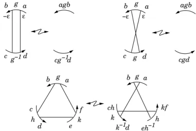
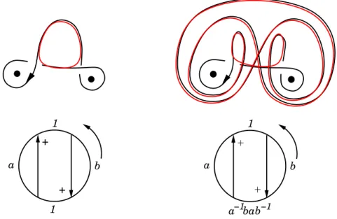
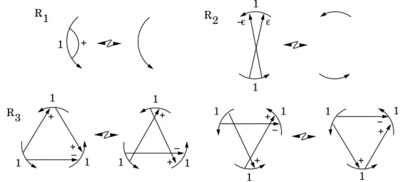
An R1-move is the local addition or removal of an isolated arrow, surrounding an edge marked with the unit 1 ∈ π. The markings of the affected edges must satisfy the rule indicated on Fig.2.8 (top-left). There are no conditions on the decorations of the arrows.
Exceptional case: If the isolated arrow is the only one in the diagram on the left,
then the markings a and b on the picture actually correspond to the same edge, and the diagram on the right, with no arrow, must be decorated by [a], the conjugacy class of a. R 2 −ε 1 R ab R 3 cd ab ε − ε 1 1 a b d c ε a 1 b a 1 1 b c d 1 1 1 1 1 1 1 1 1 1 1 1
Figure 2.8: The R-moves for Gauss diagrams on a group – the exceptional cases and the rules for the missing decorations are made precise in Definition 2.3.1.
An R2-move is the addition or removal of two arrows with opposite writhes and matching orientations as shown on Fig.2.8 (top-right). The surrounded edges must be decorated with 1, and the “merge multiply” rule should be satisfied.
Exceptional case of type 1: If the markings a and d (resp. b and c) correspond to
the same edge, then the resulting marking shall be cab (resp. abd).
Exceptional case of type 2: If the middle diagram contains no arrow at all, i.e. a
and d match and so do b and c, then the (only) marking of the middle diagram shall be [ab].
−1 a b g bg−1 g ag−1 a b cg −1 c d cg −1 c a b ag −1 g ag g b g b g d
Figure 2.9: The general conjugacy move (top-left) and its two exceptional cases – in every case the orientation of the arrow switches if and only if w(g) = −1.
An R3-move may be of the two types shown on Fig.2.8 (bottom left and right). The surrounded edges must be decorated by 1, the value of w(·)ε(·) must be the same for all three of them, and the values of ↑(·) must be pairwise distinct (see Definition 2.1.3).
A conjugacy move depends on an element g ∈ π. It changes the markings of the adjacent edges to an arbitrary arrow as indicated on Fig.2.9. Besides, if
w(g) = −1 then the orientation of the arrow is reversed – though its sign remains
the same.
Remark 2.3.2. By composing R-moves and w-moves, it is possible to perform gen-eralized moves, which look like R-moves but depend on w. Fig.2.10 shows some of
them. agb cgd ε a b d c g g −1 ε a b g ε − −1 cg d agb ε − d c g −1 −1 k kf ch k d eh b g h a a c d e f h k g b
Figure 2.10: Some generalized moves – for the R3 picture, it is assumed that ghk = 1.
Warning: the rules for the arrow orientations in R2 and R3 depend on the value of w(g).
Theorem 2.3.3. Let (Σ, x) be an arbitrary surface with a base point, and denote
a 1 − 1 correspondence between Gauss diagrams on π up to R-moves and w-moves (i.e. virtual knot types on (π, w)), and virtual knot diagrams on Σ up to diagram isotopy, Reidemeister moves and detour moves (i.e. virtual knot types on Σ).
Proof. Fix a subset X of Σ homeomorphic to a closed 2-dimensional disc and
con-taining the base point x – so that π = π1(Σ, X). Also, X being contractible allows one to fix a trivialization of the thickening of Σ over X: this gives meaning to the locally over and under branches when a knot diagram has a real crossing in X.
Construction of Φ. Pick a knot diagram D ∈ Σ and assume that every real
crossing of D lies over X. Then D defines a Gauss diagram on π, denoted by ϕ(D): the signs of the arrows are given by the writhes (Definition 2.2.3), their orientation is defined by the trivialization of M → Σ over X, and each edge is decorated by the class in π of the corresponding arc in D. This defines ϕ(D) without ambiguity if D has at least one real crossing. If it does not, then define ϕ(D) as a Gauss diagram without arrows, decorated with the conjugacy class corresponding to the free homotopy class of D. Finally, put
Φ(D) := [ϕ(D)] mod R-moves and w-moves.
Invariance of Φ under diagram isotopy and detour moves. It is clear
from the definitions that ϕ(D) is strictly unchanged under detour moves on D. Now assume that D1and D2are equivalent under usual diagram isotopy – that is, diagram isotopy that may take real crossings out of X for some time. By Corollary 2.2.9, it is enough to understand what happens for a diagram isotopy along which only one crossing goes out of X. In that case, ϕ(D) is changed by a w-move performed on the arrow corresponding to that crossing, where the conjugating element g is the loop followed by the crossing along the isotopy. Indeed, since the first Stiefel-Whitney class of the thickening of Σ coincides with that of its tangent bundle, it follows that: 1. The orientation of the fibre (and thus the notions of “over” and “under”) is
reversed along g if and only if w(g) = −1, which actually corresponds to the rule for arrow orientations in a w-move.
2. The orientation of the fibre over the crossing is reversed along g if and only if a given local orientation of Σ is reversed along g, so that the writhe of the crossing never changes.
Invariance of Φ under Reidemeister moves. Up to conjugacy by a diagram
isotopy, it can always be assumed that a Reidemeister move happens inside X. In that case, at the level of ϕ(D), it clearly corresponds to an R-move as described in Definition 2.3.1.
So far, Φ is a well-defined map from the set of virtual knot types on Σ to the set of virtual knot types on (π, w).
Construction of an inverse map Ψ. If G is a Gauss diagram without arrows,
then define ψ(G) as the totally virtual knot with free homotopy class equal to the marking of G – it is well-defined up to detour moves. If G has arrows, then for each of them draw a crossing inside X with the required writhe, and then join these
by totally virtual arcs with the required homotopy classes. The resulting diagram
ψ(G) is well-defined up to diagram isotopy and detour moves by this construction.
In both cases, put
Ψ(D) := virtual knot type of ψ(D).
Let us prove that ϕ and ψ are inverse maps, so that Ψ will be the inverse of Φ as soon as it is invariant under R-moves and w-moves.
It is clear from the definitions that ϕ ◦ ψ coincides with the identity. It is also clear that ψ ◦ ϕ is the identity, up to detour moves, for totally virtual knot diagrams.
Now fix a knot diagram D with at least one real crossing (and all real crossings inside X). Recall that ψ ◦ ϕ(D) is defined up to diagram isotopy and detour moves, so fix a diagram D′ in that class. There is a natural correspondence between the set of real crossings of D and those of D′, due to the fact that both identify by construction with the set of arrows of ϕ(D). Pick a diagram isotopy h that takes each real crossing of D to meet its match in D′, without leaving X. Then clearly ϕ(h(D)) = ϕ(D), and because ϕ ◦ ψ is the identity, one gets
ϕ(h(D)) = ϕ(D′). (2.1)
The choice of h ensures that h(D) and D′differ only by totally virtual arcs, and (2.1) implies that each of these, in h(D), has the same class in π1(Σ, X) as its match in D′, which means by definition that h(D) and D′ are equivalent up to detour moves. Thus ψ ◦ ϕ is the identity up to diagram isotopy and detour moves.
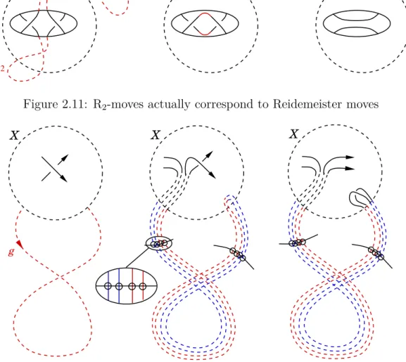
Invariance of Ψ under R-moves. Let us treat only the case of R2-moves, which contains all the ideas. Let G1 and G2 differ by an R2-move, and assume that G1 is the one with more arrows. By appropriate diagram isotopy and detour moves inside X, performed on ψ(G1), it is possible to make the two concerned crossings “face” each other, as in Fig.2.11 (left). The paths α1 and α2 from this picture are totally virtual and trivial in π1(Σ, X), thus ψ(G1) is equivalent to the second diagram of Fig.2.11 up to detour moves. The fact that at this point, an R-II move is actually possible is a consequence of (in fact equivalent to) the combinatorial conditions defining the R-moves. Denote by D the third diagram of the picture. The “merge multiply” principle that rules R2-moves implies that ϕ(D) = G2, so that
ψ(G1) ∼ D ∼ ψ ◦ ϕ(D) = ψ(G2), (2.2)
where ∼ is the equivalence under diagram isotopy, detour moves and Reidemeister moves. It follows that ψ(G1) and ψ(G2) have the same knot type.
Invariance of Ψ under w-moves. Let G1 and G2 differ by a w-move on g ∈ π. Call c the corresponding crossing on the diagram ψ(G1). Then, pick two little arcs right before c, one on each branch, and make them follow g by a detour move. At the end, one shall see a totally virtual 4-lane railway as pictured on Fig.2.12 (middle): the strands are made parallel, i.e. any (virtual) crossing met by either of them is part of a larger picture as indicated by the zoom. This ensures that, using the mixed version of Reidemeister III moves, one can slide the real crossing all along the red part of the railway, ending with the diagram on the right of the picture – let us call
α2
α1
X X X
Figure 2.11: R2-moves actually correspond to Reidemeister moves X
X
g
X
Figure 2.12: Performing a w-move – the railway trick
it D. The conclusion is identical to that for R-moves: again ϕ(D) = G2 and (2.2) holds, whence ψ(G1) and ψ(G2) have the same knot type.
About the orbits of w-moves
It could feel natural to try to get rid of w-moves by understanding their orbits in a synthetic combinatorial way. This is what is done in Section 2.3.2 in the particular case of an abelian group π endowed with the trivial homomorphism π → F2.
In general, for a Gauss diagram on π, G, denote by h1(G) the set of free homotopy classes of loops in the underlying topological space of G (it is the set of conjugacy classes in a free group on deg(G) + 1 generators). Also, denote by h1(π) the set of conjugacy classes in π. Then the π-markings of G define a map
FG: h1(G) → h1(π).
questions that amout to technical group theoretic problems, and which will not be answered here (Gw denotes the orbit of G under w-moves):
1. Is the map Gw 7→ F
G injective?
2. If the answer to 1. is yes, then is Gw determined by a finite number of values
of FG, for instance its values on the free homotopy classes of simple loops?
3. Is it possible to detect in a simple manner what maps h1(G) → h1(π) lie in the image of Gw 7→ F
G?
Remark 2.3.4. Gauss diagrams with decorations in h1(Σ) can be met for example in [15], where they are used to construct knot invariants in a thickened oriented surface Σ – see Section 3.4. If the answer to Question 1. above is no, then such invariants, which factor through FG, stand no chance to be complete.
Remark 2.3.5. Even for diagrams with only one arrow, it still does not seem easy to
answer the “simple loop” version of Question 2. Given x, y, h, k in a finite type free group, is it true that
hxh−1kyk−1= xy =⇒ ∃l,
(
hxh−1 = lxl−1 kyk−1 = lyl−1 ?
Let us end with an example that shows that the values of FG on the (finite) set
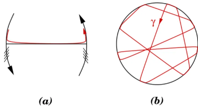
of simple loops running along at most one arrow is not enough (cf. Question 2.). Fig.2.13 shows a Gauss diagram with such decorations – {a, b} is a set of generators for the free group π1(Σ) ≃ F(a, b), where Σ is a 2-punctured disc. These particular values of FG do not determine the free homotopy class of the red loop γ, as it is
shown in Fig.2.14. [a] [b] + [ab] γ [b] [a] +
Figure 2.13: A Gauss diagram that does not define a unique virtual knot In fact, these two virtual knots are even distinguished by Vassiliev-Grishanov’s planar chain invariants, which means they represent different virtual knot types.
2.3.2 Abelian Gauss diagrams
In this subsection, π is assumed to be abelian, and w0 denotes the trivial homo-morphism π → F2. We describe a version of Gauss diagrams that carries as much information as the previously introduced virtual knot types on (π, w0), with two improvements:
+ + 1 b a 1 + + −1 −1 a bab b a 1
Figure 2.14: One red loop is trivial, while the other is a commutator ➺ This version is free from conjugacy moves.
It is inspired from the decorated diagrams introduced by T. Fiedler to study combi-natorial invariants for knots in thickened surfaces (see [9, 10]).
We use the same notation G for a Gauss diagram and its underlying topological space, that is a 1-dimensional complex with edges and arrows as oriented 1-cells.
H1(G) denotes its first integral homology group.
Definition-Lemma 2.3.6 (fundamental loops). Let G be a classical Gauss diagram
of degree n. There are exactly n + 1 simple loops in G respecting the local orienta-tions of edges and arrows, and going along at most one arrow. They are called the
fundamental loops of G and their homology classes form a basis of H1(G).
Definition 2.3.7 (abelian Gauss diagram). Let π be an abelian group. An abelian
Gauss diagram on π is a classical Gauss diagram G decorated with a group
homo-morphism µ : H1(G) → π. It is usually represented by its values on the basis of fundamental loops, that is, one decoration in π for each arrow, and one for the base circle – that last one is called the global marking of G.
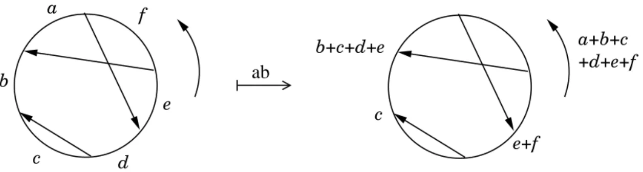
A Gauss diagram on π determines an abelian Gauss diagram as follows: ➺ The underlying classical Gauss diagram is the same.
➺ Each fundamental loop is decorated by the sum of the markings of the edges that it meets (see Fig 2.15).
This defines an abelianization map ab.
Proposition 2.3.8. The map ab induces a natural 1 − 1 correspondence between
abelian Gauss diagrams on π and equivalence classes of Gauss diagrams on π up to w0-moves. Moreover, if π = π1(Σ) is the fundamental group of a surface, then these sets are in 1 − 1 correspondence with the set of virtual knot diagrams on Σ up to diagram isotopy and detour moves.
Proof. The proof of the last statement is contained in that of Theorem 2.3.3 –
a+b+c +d+e+f a f e d c b c e+f b+c+d+e ab
Figure 2.15: Abelianizing a Gauss diagram on an abelian group
isotopy, and that w-moves at the level of knot diagrams can be performed using only detour moves and diagram isotopies, by the railway trick (Fig.2.12).
As for the first statement, one easily sees that ab is invariant under w0-moves. We have to show that conversely, if ab(G1) = ab(G2), then G1 and G2 are equivalent under w0-moves.
This is clear if G1 has no arrows, since then ab(G1) = G1. Now proceed by induction. Since G1 and G2 have the same abelianization, they have in particular the same underlying classical Gauss diagram, and there is a natural correspondence between their arrows.
Case 1: No two arrows in G1cross each other. Then at least one arrow surrounds a single isolated edge on one side (as in an R1-move). Choose such an arrow α and remove it, as well as its match in G2. By induction, there is a sequence of w0-moves on the resulting diagram G′
1 that turns it into G′2. Since the arrows of G′1 have a natural match in G1, those w0-moves make sense there, and take every marking of G1 to be equal to its match in G2, except for those in the neighborhood of α. So we may assume that G1 and G2 only differ near α as in Fig.2.16. Since all the unseen markings coincide in G1 and G2, and since ab(G1) and ab(G2) have the same global marking, it follows that
a+ b + c = a′+ b′+ c′.
Thus a w0-move on α with conjugating element g = a′− a turns G1 into G2.
a b c ’ ’ ’ 2 G a b c G 1 α α
Figure 2.16: Notations for case 1
Case 2: There is at least one arrow α in G1 that intersects another arrow. By the same process as in case 1, one may assume that G1 and G2 only differ near α – see Fig.2.17, where a, b, c and d actually correspond to pairwise distinct edges since
one obtains
a+ d = a′+ d′,
and
b+ c = b′+ c′,
by considering the global marking, and the marking of α, in ab(G1) and ab(G2). Moreover, there is at least one arrow intersecting α: considering the marking of that arrow gives
a+ b = a′+ b′.
The last three equations may be written as
a′− a = b − b′ = c′ − c= d − d′,
so that, again, a w0-move on α with conjugating element g = a′− a turns G1 into G2. 2 G G 1 α a b c d α a b c d ’ ’ ’ ’
Figure 2.17: Notations for case 2
Remark 2.3.9. Another proof of this proposition was given in a draft paper, in the
special case π = Z ([21], Proposition 2.2). As an exercise, one can show that this proof extends to the case of an arbitrary abelian group.
To make the picture complete, it only remains to understand R-moves in this context.
Definition 2.3.10 (obstruction loops). Within any local Reidemeister picture like
those shown on Fig.2.4 featuring at least one arrow, there is exactly one (unoriented) simple loop. We call it the obstruction loop. Fig.2.18 shows typical examples.
Definition 2.3.11 (R-moves). A move from Fig.2.4 is likely to define an R-move
only if the obstruction loop lies in the kernel of the decorating map H1(G) → π (which makes sense even though the loop is unoriented). Under that assumption,
the R-moves for abelian Gauss diagrams are defined by the usual conditions: ➺ i= 1. No additional condition.
➺ i= 2. The arrows head to the same edge, and have opposite signs.
➺ i= 3. The value of w(e)ε(e) is the same for all three visible edges e, and the values of ↑(e) are pairwise different (see Definition 2.1.3).
R 2 1 R R 3
Figure 2.18: Homological obstruction to R-moves
Theorem 2.3.12. The map ab induces a natural 1 − 1 correspondence between
equivalence classes of abelian Gauss diagrams on π up to R-moves and virtual knot types on (π, w0).
Proof. ab clearly maps an R-move in the non commutative sense to an R-move in
the abelian sense. Conversely, if ab(G1) and ab(G2) differ from an (abelian) R-move, then the vanishing homological obstruction implies that G1 and G2 are in a position to perform a “generalized R-move” like the examples pictured on Fig.2.10.
Theorems 2.3.3 and 2.3.12 together imply the following
Corollary 2.3.13. If Σ is an orientable surface with abelian fundamental group,
then there is a 1 − 1 correspondence between abelian Gauss diagrams on π1(Σ) up to R-moves, and virtual knot types on Σ.
2.3.3 Homological formulas
It may seem not easy to compute an arbitrary value of the linear map decorating an abelian Gauss diagram, given only its values on the fundamental loops. To end this section, we give two formulas to fill this gap, by understanding the coordinates of an arbitrary loop in the basis of fundamental loops.
The energy formula
Fix an abelian Gauss diagram G. Observe that as a cellular complex, G has no 2-cells, thus every 1-homology class has a unique set of “coordinates” along the family of edges and arrows. For each 1-cell c (which may be an arrow or an edge), we denote by h·, ci : H1(G) → Z the coordinate function along c. It is a group homomorphism.
Let us denote by [A] ∈ H1(G) the class of the fundamental loop associated with an arrow A (Fig.2.19 left).
Definition-Lemma 2.3.14 (Energy of a loop). Fix an edge e in G, and a class γ ∈ H1(G). The value of Ee(γ) = hγ, ei − X h[A],ei=1 hγ, Ai (2.3)
is independent of e. This defines a group homomorphism E : H1(G) → Z.
Proof. Let us compare the values of E·(γ) for an edge e and the edge e′ right after it. e and e′ are separated by a vertex P , which is the endpoint of an arrow A. There are two possible situations (Fig.2.19):
1. P is the tail of A. Then h[A] , ei = 1 and h[A] , e′i= 0, so that Ee(γ) − Ee′(γ) = hγ, ei − hγ, Ai − hγ, e′i .
2. P is the head of A. Then h[A] , ei = 0 and h[A] , e′i= 1, so that Ee(γ) − Ee′(γ) = hγ, ei + hγ, Ai − hγ, e′i .
In both cases, Ee(γ) − Ee′(γ) is equal to h∂γ, P i, which is 0 since γ is a cycle.
e
e’
A
A
[A]
e
e’
[A]
A
[A]
Figure 2.19: The fundamental loop of an arrow and the two cases in the proof of Lemma 2.3.14
Theorem 2.3.15. For any γ ∈ H1(G), one has the decomposition γ =X
A
hγ, Ai[A] + E(γ) [K] . (2.4)
Proof. This formula is an identity between two group homomorphisms, so it suffices
to check it on the basis of fundamental loops, which is immediate.
Remark 2.3.16. The existence of a map E such that Theorem 2.3.15 holds was clear,
since for each arrow A considered as a 1-cell, [A] is the only fundamental loop that involves A. With that in mind, one may read into (2.3) as follows: E(γ) counts the (algebraic) number of times that γ goes through an edge, minus the number of those times that are already taken care of by the fundamental loops of the arrows. This number has to be the same for all edges, so that one recovers a multiple of [K].