Data mining for diagnosis, monitoring, and prediction in wind
power plants
by
Mostafa SAEIDI
THESIS PRESENTED TO ÉCOLE DE TECHNOLOGIE SUPÉRIEURE
IN PARTIAL FULFILLMENT FOR A MASTER’S DEGREE
WITH THESIS IN ELECTRICAL ENGINEERING
M.A.Sc.
MONTREAL, 14TH AUGUST 2020
ÉCOLE DE TECHNOLOGIE SUPÉRIEURE UNIVERSITÉ DU QUÉBEC
© Copyright reserved
It is forbidden to reproduce, save or share the content of this document either in whole or in parts. The reader who wishes to print or save this document on any media must first get the permission of the author.
BOARD OF EXAMINERS (THESIS M.SC.A.)
THIS THESIS HAS BEEN EVALUATED BY THE FOLLOWING BOARD OF EXAMINERS
Mr. Ambrish Chandra, Thesis Supervisor
Département de génie électrique at École de technologie supérieure
Mr. Zhaoheng Liu, President of the Board of Examiners
Département de Génie Mécanique at École de technologie supérieure
Mr. Pierre Jean Lagacé, Member of the jury
Département de génie électrique at École de technologie supérieure
Mr. Philippe Cambron, External Evaluator Power Factors
THIS THESIS WAS PRENSENTED AND DEFENDED
IN THE PRESENCE OF A BOARD OF EXAMINERS AND PUBLIC <DEFENCE DATE OF THE THESIS>
ACKNOWLEDGMENT
It is a pleasure to thank the many people who have helped and inspired me during my M.A.Sc. study. First of all, I would like to express my deep and sincere gratitude to my supervisor, Ambrish Chandra. His understanding, encouraging and personal guidance have provided a fundamental basis for the present thesis. His patience, guidance, encouragement, and useful critiques through this research work helped me enormously. Many thanks also to Dariush Faghani, Phippe Cambron, and Francis Pelletier from Power Factors. Their detailed and constructive advices helped me in the development of my team working and professionalism skills and this work. I would like to thank the members of my examining committee: Pierre Jean Lagacé, Philippe Cambron, and Zhaoheng Liu, who have agreed in evaluating this thesis and provided me valuable comments. Thanks also to my many colleagues in the GREPCI (le Groupe de recherche en électronique de puissance et commande industrielle) who provided a stimulating and friendly environment to learn and grow. Also, I would like to give my special thanks to my entire family and parents, Mohammadreza and Farahnaz for providing me with unfailing support and continuous encouragement throughout my years of study. Most of all, thanks to my dearest friend, Pardis for her understanding, endless love, and encouragement which were fundamental for me during my study. They have always supported, inspired, and loved me. To all of them I dedicate this thesis. I also thank National Sciences and Engineering Research Council NSERC of Canada, and École de Tecnologie Supérieure for their financial support. This work would not have been possible without their support.
Extraction de données pour le diagnostic, la surveillance et la prévision dans les centrales éoliennes
Mostafa SAEIDI
RÉSUMÉ
De nos jours, les sources d'énergie renouvelables jouent un rôle clé dans l'ingénierie des systèmes électriques. Parmi la multiplicité des sources d'énergie, l’énergie éolienne est plus populaire en raison de ses avantages substantiels tels que le bas coût de l’énergie produite, sa technologie bien établie et le fait qu'elle soit plus accessible. Cependant, ce type de technologies a des coûts considérables qui peuvent réduire les bénéfices des investisseurs et des consommateurs. Parmi les différents coûts, les coûts d'exploitation et de maintenance jouent un rôle clé, car de nombreuses éoliennes installées vieillissent. Pour réduire les coûts d’exploitation et d’entretien, il est essentiel d’actualiser les stratégies définies pour la surveillance de l’état dans les parcs éoliens. L’outil de surveillance de l’état approprié doit être développé après avoir effectué une étude complète des techniques de surveillances de l’état existantes. Pour passer d’une surveillance de l’état manuelle à une approche automatique et intelligente, les concepts d’apprentissage automatique et d’exploration de données seront utilisés dans cette application. La nécessité d’une stratégie moderne de surveillance de l’état coïncide avec l’émergence de l’apprentissage en profondeur au cours de la dernière décennie. Une nouvelle surveillance de l’état est proposée dans cette thèse, afin de surveiller la température des enroulements des générateurs dans un parc éolien, en utilisant le modèle de mémoire à court terme qui est une méthode de réseau de neurones récurrents. Ce modèle d’apprentissage en profondeur est un choix pratique et unique pour la prédiction en raison de sa capacité à prendre en compte les dépendances à long terme entre les caractéristiques séquentielles d’entrée qui, dans ce cas, sont l’ensemble des données chronologiques fournies par le système SCADA. Les données chronologiques de SCADA sont fournies par Power Factors qui dispose d'une vaste base de données d'informations sur les performances des différentes centrales électriques, qui a été rassemblée par un système SCADA à une fréquence de 1 Hz. Le nouveau modèle proposé dans cette thèse est évalué à partir d’un parc éolien dans la province de Québec (Canada), où les scénarios de cas seront des conditions de fonctionnement sain et anormal. De plus, le signal d’erreur est calculé entre les signaux réels et prédits pour évaluer la bonne performance du modèle. Enfin, ce modèle est comparé avec le modèle de régression linéaire multiple pour montrer l’efficacité et la grande précision du modèle proposé.
Mots-clés: surveillance de l'état, mémoire à court terme, SCADA, apprentissage en
Data mining for diagnosis, monitoring, and prediction in wind power plants
Mostafa SAEIDI
ABSTRACT
Nowadays, renewable energy sources play the key role in power system engineering. Among multiplicity of energy sources, wind energy is more popular due to its substantial advantages such as lower prices of produced electricity, their established technology, and being more accessible. However, these technologies have considerable costs that can mitigate profit for the investors and consumers. Among the different costs, the operation and maintenance (O&M) costs have the key role since many installed wind turbines are getting older. To mitigate the O&M costs it is crucial to update the defined strategies for condition monitoring (CM) in wind farms. The proper CM tool should be developed after exerting complete survey of existing CM techniques. To shift from a manual CM toward an automatic and smart approach, the machine learning and data mining concepts will be utilized in this application. The need for a modern condition monitoring strategy coincides with the emergence of Deep Learning (DL) in the recent decade. In this thesis, a novel condition monitoring is proposed to monitor the temperature of generator windings in a wind farm using Long Short-Term Memory (LSTM) model which is a Recurrent Neural Network (RNN) method. This DL model is a practical and unique choice for prediction due to its ability for considering long-term dependencies among input sequential features, which in this case are the provided time-series datasets by SCADA system. The time-series SCADA datasets are provided by Power Factors which has a vast database of information about performance of different power plants which is gathered by SCADA system at 1Hz frequency. The novel proposed model in this thesis is evaluated in healthy and abnormal operation modes of a wind farm in Quebec Province, Canada as case scenarios. Moreover, the error signal is calculated between real and predicted signals to evaluate the proper performance of the model. Finally, this model is compared with Multiple Linear Regression model to show the effectiveness and high precision of the proposed model.
Keywords: condition monitoring, long short-term memory, SCADA, deep learning, generator
TABLE OF CONTENTS
Page
INTRODUCTION ...16
CHAPTER 1 Problem Description ...19
1.1 Supervisory Control and Data Acquisition (SCADA) systems ...20
1.2 Condition monitoring challenges of wind power plants ...21
1.3 Objectives of project ...23
1.4 Research Contribution ...24
1.5 Methodology ...25
1.5.1 A thorough literature review ... 25
1.5.2 Refining raw data ... 26
1.5.3 Pre-interpretation of data based on grid codes ... 26
1.5.4 ML usage for interpretation of data ... 27
CHAPTER 2 Literature Review...28
2.1 Common failures in main equipment ...28
2.1.1 Blades ... 29 2.1.2 Gearbox ... 29 2.1.3 Main Shaft ... 29 2.1.4 Power Converters ... 30 2.1.5 Electric Machine ... 30 2.2 Spectral Analysis ...31 2.3 Signal Trending ...35 2.4 Physical Model...36
2.5 ML and signal processing techniques ...38
CHAPTER 3 Proposed Data Preprocessing Technique and Regression Model ...41
3.1 Correlation Analysis ...41
3.2 Multiple Linear Regression (MLR) ...42
3.3 Artificial Neural Network (ANN) ...44
3.3.1 Activation Function ... 45
3.3.1.1 Binary Step Function ... 45
3.3.1.2 Linear Activation Function ... 46
3.3.1.3 Sigmoid Function ... 47
3.3.1.4 Hyperbolic Tangent Function ... 48
3.3.2 Optimizer ... 49
3.3.3 Loss Function ... 50
3.3.4 Learning Rate ... 52
3.3.5 Dropout ... 52
3.4 Recurrent Neural Network (RNN) ...54
3.4.1 Vanishing Gradient Challenge: ... 55
CHAPTER 4 Results & Discussions...61 4.1 Stacked LSTM ...61 4.2 Bidirectional LSTM ...67 4.3 Multivariate LSTM ...69 4.4 Performance Comparison...77 CONCLUSION ...80 RECOMMANDATIONS ...81
LIST OF TABLES
Page
Table 0.1 Number of wind turbine and installed wind power : Canada & Quebec ...21
Table 0.2 O&M costs in Canada ...33
Table 2.1 Carrier frequencies (CF) and their side-bands ...33
Table 4.1 The candidate parameters for inputs and output ...70
Table 4.2 Correlation values of candidate parameters ...71
Table 4.3 Tuned hyperparameters for developed LSTM models ...78
LIST OF FIGURES
Page
Figure 0.1 Installed wind power plant capacity in Canada ...16
Figure 1.1 Structure of a SCADA system ...76
Figure 1.2 Time trace of substation voltage ...23
Figure 1.3 The flowchart of project methodology ...25
Figure 2.1 Failure rate in wind power plant components ...28
Figure 2.2 Common failure rate in power converters of wind power plants ...30
Figure 2.3 The stator current spectrum ...32
Figure 2.4 The stator current spectrum in different operational condition ...34
Figure 2.5 The spectrum of active power in different operation condition ...34
Figure 2.6 Drive train temperature ...35
Figure 2.7 The gathered raw data by SCADA system for 750 kW wind turbine ...36
Figure 2.8 Pre-processed data for a 750-kW wind turbine ...37
Figure 2.9 Generator winding fault detection ...38
Figure 3.1 Correlation scenarios between two variables ...42
Figure 3.2 The topology of a one-layer ANN ...44
Figure 3.3 A graphical representation of neuron structure ...45
Figure 3.4 Binary step activation function representation ...46
Figure 3.5 Linear activation function representation ...46
Figure 3.6 Sigmoid activation function representation ...47
Figure 3.7 Hyperbolic tangent activation function ...48
Figure 3.9 Learning rate effect on finding the optimal point ...52
Figure 3.10 Dropout implementation on an ANN ...53
Figure 3.11 RNN topology over time ...54
Figure 3.12 Simple LSTM structure...56
Figure 3.13 LSTM structure ...57
Figure 4.1 Generator windings actual temperature: WT 7 ...62
Figure 4.2 Generator windings actual temperature: WT 67 ...62
Figure 4.3. Training dataset: Generator Winding Temperature WT 7 ...64
Figure 4.4. Testing dataset: Generator Winding Temperature WT 7 ...65
Figure 4.5 Predicted generator windings temperature by Stacked LSTM: WT 7 ...66
Figure 4.6 Predicted generator windings temperature by Stacked LSTM: WT 67 ...66
Figure 4.7 Bidirectional LSTM structure ...67
Figure 4.8 Predicted target variable by Bidirectional LSTM: WT 7 ...68
Figure 4.9 Predicted target variable by Bidirectional LSTM: WT 67 ...69
Figure 4.10 Scatter plots of candidate parameters ...71
Figure 4.11 Generator cooling system temperature: WT 7 ...72
Figure 4.12 Produced active power: WT 7 ...73
Figure 4.13 Generator cooling system temperature: WT 67 ...73
Figure 4.14 Produced active power: WT 67 ...74
Figure 4.15 Predicted target variable by Multivariate LSTM: WT 7 ...75
Figure 4.16 Predicted target variable by Multivariate LSTM: WT 67 ...75
Figure 4.17 Histogram of model residuals ...75
Figure 4.18 Density plot of model residuals ...75
LIST OF ABREVIATIONS
RES Renewable Energy Source
O&M Operation and Maintenance
AC Alternating Current
DC Direct Current
SCADA Supervisory Control and Data Acquisition RTU Remote Terminal Units
PLC Programmable Logic Control LSTM Long Short-Term Memory
PMSG Permanent Magnetic Synchronous Generator MPPT Maximum Power Point Tracking
DFIG Doubly-Fed Induction Generator RNN Recurrent Neural Network MLR Multiple Linear Regression ANN Artificial Neural Network NLP Natural Language Processing
MLP Multi-Layer Perception
SGD Stochastic Gradient Descent
GD Gradient Descent
ADAM Adaptive Moment Estimation MSE Mean Square Error
MAE Mean Absolute Error
NEMA National Electrical Manufacturers Association CNN Convolutional Neural Network
LIST OF SYMBOLS
𝑘 Harmonic index
𝑓 Supplying frequency of induction machine 𝑠 Slip
𝑓 Broken rotor bar harmonic frequency 𝑓 Stator windings harmonic frequency
𝑓 Faulty frequency related to unbalanced rotor in induction machines 𝑝 Number of pole pairs
𝑙 Supply time harmonic constant
𝑓 Supplying frequency
𝑥 Input feature of models
𝑦 Dependent variable or target variable 𝑥̅ Mean value of input feature
𝑦 Mean value of dependent variable
𝛽 Regression coefficient
𝜀 Error of model
𝑟 Correlation between x and y variables 𝜎 Sigmoid activation function
Tanh Tangent hyperbolic activation function 𝐸(𝑘) Prediction error vector at time step k 𝑐 Cell state or memory state
ℎ Output of LSTM model 𝑊 Vector of weights
𝑊 Vector of weights for input features
𝑊 Vector of weights for previous LSTM cell output
INTRODUCTION
In recent decades, renewable energy sources (RESs) have been the focal point of research among scholars due to their considerable advantages over conventional and fossil fuel-based power plants. Penetration of RESs has been increased substantially in power network in recent decade to provide both consumers and network operators with technical and economic benefits. Technological development of power electronics has also boosted RESs utilization in both transmission and distribution levels of power network (Garcia-Vera, Dufo-Lopez & Bernal-Agustin, 2019). In recent decade, Canadian government has increased the investment in RES. Currently, Canada is ranked 9th in global wind power generation by producing 2% of global
wind power generation and 4% of Canada’s electricity generation (Canadian Wind Energy Association, 2020). In Figure 0.1, the increase in installed capacity of wind power plants in Canada is shown.
Figure 0.1 Installed onshore wind power plant capacity in Canada Taken from CanWEA (2020)
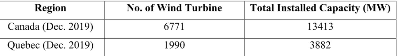
It is obvious from Figure 0.1 that by the end of 2019, more than 13GW wind power is installed all over Canada and wind power plants have a high share of power production in the network. Besides, the number of installed turbines has been also increased in Canada and Quebec. In Table 0.1, the numbers of turbines and installed wind power capacity in Canada and Quebec are presented (CanWEA, 2020).
Table 0.1 Number of wind turbine and installed wind power: Canada and Quebec
Region No. of Wind Turbine Total Installed Capacity (MW)
Canada (Dec. 2019) 6771 13413
Quebec (Dec. 2019) 1990 3882
Many of these turbines are installed more than 10 years ago and precise condition monitoring strategies should be implemented for them to prevent any failure in the system. It is worth mentioning that the O&M expenses in wind power industry are increasing considerably. Table 0.2 shows the increasing trend of O&M costs in Canada (Canadian wind Energy Association, 2017).
Table 0.2 O&M costs in Canada
Year O&M (M$)
2017 290 2020 450
According to Table 0.2, it is anticipated that the O&M costs of wind power plants in Canada will increase to 450M$ by the end of 2020 (CanWEA, 2017). Hence, scholars in collaboration with wind industry are trying to find innovative ways to decrease O&M costs in recent years. The scope of this research is to develop a powerful tool for fault diagnosis, condition monitoring, and fault prediction for wind power plants (specifically for generator windings) in collaboration with Power Factors and Natural Sciences and Engineering Research Council (NSERC). The rest of this report is organized as follows:
• Chapter 1 defines the problem and motivation for solving it. Objectives of project and the expected contributions are discussed in this chapter.
• Chapter 2 expounds the previous works on condition monitoring in wind power plants. Furthermore, an overview on Machine Learning (ML) and Deep Learning (DL) usage for processing SCADA data is provided in this chapter.
• Chapter 3 explains detailed methodology of project for achieving the defined goals and elaborates the concepts, advantages, and disadvantages of Multiple Linear Regression, Artificial Neural Networks, Recurrent Neural Network, Long Short-Term Memory. Moreover, the concept of Correlation Analysis for feature selection is explained.
• Chapter 4 defines two case scenarios which represents the healthy and faulty operation modes of a wind farm in the North of Quebec Province, Canada. The provided datasets by Power Factors are preprocessed and after implementing Correlation Analysis, the chosen input features are fed to different types of LSTM models in order to predict the generator winding temperature in both case scenarios. Finally, the obtained results are compared to indicate the performance of model. In the final section, a conclusion from this thesis is provided and some possible ideas for future works are discussed.
CHAPTER 1
PROBLEM DESCRIPTION
In last decade, electricity usage in urban and rural areas is increased substantially. Considering the electricity history, AC generators gained much more attention based on their abilities over DC generators. Most of the primitive power plants were diesel and steam generators; however, steam and hydro power plants widely added to power networks after a while. The increasing penetration of fossil fuel-based power plants in power grid have raised many environmental concerns which coerces many to see RES as a unique solution for meeting the electricity demand while considerably decreases Co2 emission (Østergaard et al., 2020).
Wind power plants among different RESs have more established technology which made them more popular. Moreover, the energy source is free in these power plants which make them one of the affordable RESs. Besides all the merits that wind power plants have, it should be noted that their presence in power grid creates challenges for grid operators and owners of wind power plants. The intermittent production of power (due to unpredictable nature of wind speed) needs specific control algorithms and considerations that are not taken into account for fossil fuel-based power plants.
Another equally noteworthy challenge in operation of wind power plants is their considerable maintenance expenses. For several years, RESs have been advertised as cutting-edge technologies; however, after passing 20 years from their operation in power network, they cannot be considered as new technologies anymore. More equipment in wind power plants is reaching the end of their life span (Papatzimos et al., 2019). As a result, the O&M costs are increasing substantially in recent years. It has been anticipated that by the end of 2020, over 450 M$ is needed for O&M costs of wind industry in Canada (CanWEA, 2017). Hence, it is highly important for governments and wind power plants owners to keep their competitiveness with fossil fuel-based power plants. Considering high share of O&M costs in total expenses of
power plants, finding solutions for reducing O&M costs of wind power plants will be the best way to increase the competitiveness of these power plants.
1.1 Supervisory Control and Data Acquisition (SCADA) systems
It is worth mentioning that Supervisory Control and Data Acquisition (SCADA) systems are widely used in wind power plants to gather data from equipment and send them to command center for processing and operation. The gathered data by SCADA systems can be used for monitoring the system operation. In the Fig. 1.1, it has been illustrated how SCADA system works (Inductive Automation, 2018).
The installed sensors, all over the wind power plant, gather data and send them to programmable logic controllers (PLCs) or remote terminal units (RTUs). Data can be sent to PLCs and RTUs manually, as well. PLCs and RTUs convey the gathered data to SCADA system for further actions. In the next step, SCADA systems prepare data for supervisory and
Figure 1.1 Structure of a SCADA system Taken from Inductive Automation (2018)
operational actions (Setiawan et al., 2018). Usually SCADA systems gather the data from different equipment by 10-mins average. However, SCADA systems are capable of gathering data for higher frequency up to 1 Hz. It is worth mentioning that 10-mins average gathering of data make analyzing system parameters more complex, especially for electrical parameters which usually have faster variations than mechanical ones.
1.2 Condition monitoring challenges of wind power plants
Considering the fact that studying horizon (which can be over 10 years) is much bigger than the gathering sample rate (in our case it is 10-mins average), the gathered data will be enormous over the years and as a result, their analysis will be a time-consuming process. The raw data which are gathered by SCADA systems provide the operators with several challenges that should be considered to guarantee proper operational analysis of wind power plants. These challenges can be explained as follows:
• Many of the gathered data may be out of rational operational boundaries. These data can affect proper condition monitoring analysis and moreover, the time required for analysis will be increased significantly. Hence, the raw data should be pre-processed based on the elimination these data (Yang & Shen, 2020).
• Any failure in measurement systems can affect the gathered data. It is highly important to know that the data have been gathered and processed under healthy operation of sensors, PLCs, and RTUs. By knowing the failure report of measurement devices, the faulty data can be deleted from our dataset (Jiang & Srivastava, 2020).
• Condition monitoring analysis is significantly related to the system operation point. Considering the fact that operation point of wind power plants is more variable than fossil fuel-based power plants (due to their dependence on wind speed), it can be deduced that condition monitoring in wind power plants are more complicated.
• The wind power plants experience shut-down periods due to different reasons such as grid operators command, curtailment, high wind speed and etc. The shut-down periods produce blank data in the database which affect the continuity of condition monitoring analysis.
• Another challenge in analyzing SCADA data for wind power plants is mutual interactions between mechanical and electrical parameters. This correlation fails any successful individual investigation for electrical or mechanical data analysis. Hence, any specific parameter monitoring in these systems needs more complicated control algorithms to consider the correlation between mechanical and electrical parameters (Moeini et al., 2019).
• The other challenge for condition monitoring in wind power plants is the geographical position of turbines. It is very important to consider the turbines’ location in the condition monitoring, because the wind speed, shading effects, ambient temperature, altitude, and etc. are several parameters that related to the geographical position of turbines which affect the generated power (Aziz et al., 2019), (Shen et al., 2019), (Patrizi, Ciani, Guidi & Bartolini, 2019).
These challenges should be considered in developing any condition monitoring tool for wind power plants. To show the complexities of these challenges in the time trace of real data, the voltage of a wind power plant in high voltage side of its substation is shown in Fig. 1.2.
This wind power plant is located in Quebec Province, Canada and the data is provided in collaboration with Power Factors; however, the name of this power plant is not mentioned here due to confidentiality reasons. The nominal voltage at high voltage side of substation is 161 kV. From Fig. 1.2, it can be understood that most of gathered data deviate around 161 kV, which is the nominal voltage at the high voltage side of substation. However, there are many data which is below 140 kV and many periods have zero voltage. The root cause of these considerable deviations can be any of the mentioned challenges.
1.3 Objectives of project
In order to reduce the O&M costs of wind power plants, there is a need for an accurate condition monitoring tool to overcome mentioned challenges and also reduce operational costs
of wind power plants. This goal cannot be achieved without exploiting ML techniques. As a result, the main objective of this project is to develop a precise condition monitoring tool for monitoring the temperature of generators’ windings in wind power plants by using the gathered data from SCADA systems and using data mining and ML techniques for processing them.
1.4 Research Contribution
As it was mentioned earlier, few works have focused on electrical side of condition monitoring in wind power plants and mechanical equipment such as gearbox, blades, bearings and etc. were the focal point of research in recent decades. Hence, any endeavor for monitoring electrical equipment can be a contribution. Furthermore, since this project is in collaboration with an industrial compartment (Power Factors), it is important to know that there are several practical contributions for this project beside the research contributions.
In this project a diagnosis/monitoring/predictive tool is developed by DL approach for integrating to Power Factors’s DIAGNOSTIX tool. Therefore, the development of this type of tool will help the electric power industry, in general and help Power Factors to keep its competitive edge at national and global market and benefit several industries in renewable energy sources areas, as well.
In the following, several research contributions of this project are explained:
• In this project, mutual investigation of electrical and mechanical parameters will be the focal research point. Moreover, the correlation analysis will be performed between mechanical and electrical parameters of system to extract exact relations between different parameters.
• Another contribution of this project is anomaly detection in the provided parameters by early prediction of faults and malfunction in the system. This will give the owners of wind power plants a unique opportunity to prevent any damage to their equipment.
• The main contribution of this project is implementing ML techniques for monitoring the temperature of generator windings based on the gathered real data from SCADA systems. Since the provided temperature signal is time-series data, Long Short-Term Memory (LSTM) technique is the best method for developing a monitoring model. Besides, a comprehensive literature review on ML applications on wind farm maintenance will be provided.
1.5 Methodology
To reach the mentioned goal in the previous chapter, it is important to propose a well-organized and detailed methodology. In the following, the methodology of this research is demonstrated in a flowchart.
The methodology has been proposed in several steps as follows:
1.5.1 A thorough literature review
Similar to every other project, it is necessary to perform a complete literature survey about the problem in order to gather required knowledge. The main focus on this project will be on two topics as follows:
• It is necessary in the first step to review the works that have been done on condition monitoring for equipment of wind power plants. Although most of the works has only focused only individual equipment for condition monitoring, these papers give good insight about the most common failures in them.
• Another equally noteworthy topic for literature review is the methods that have been used by papers for processing the gathered data by SCADA systems. The main focus in this part will be on the ML and data mining techniques which are used for processing the data and early stage prediction of faults in the system.
1.5.2 Refining raw data
As it was mentioned earlier, the gathered data by SCADA system can be logically false due to various reasons such as sensor failures, shut-down periods, and etc. It is crucial to exert a refining operation on these data before using them for further condition monitoring analysis and refining operation is called “pre-processing” the data. The main focus on preprocessing the data is to delete those data that are logically false. As an example, the amplitude of depicted substation voltage in Fig. 1.2. cannot be negative; hence, any negative voltage in the database should be eliminated to guarantee proper further analysis.
1.5.3 Pre-interpretation of data based on grid codes
It should be noted that each of the equipment that have been used in wind power plants can operate within ranges for normal operation or transient operation (when a fault occurs in the main grid or other parts of power plant). Moreover, the grid operators define various regulations in order to satisfy different indices to guarantee proper delivery of electrical energy to costumer. These regulations are known as grid codes which in this project are defined by Hydro-Quebec as the grid operator in Quebec Province. The grid codes will be scrutinized in literature review section.
After refining the gathered data in previous part, it is important to exert a pre-processing analysis based on the existing grid codes and defined operational ranges for each of the parameters. This will give us a good sight about the faulty and healthy operation regions. Moreover, it can be seen how close the system is operating to defined boundaries.
1.5.4 ML usage for interpretation of data
After determining the healthy operation regions, the dataset will be ready for being processed by ML methods in order to move from manual condition monitoring, which was based on data checking with grid codes and normal operation ranges, to a smart condition monitoring method which is not only shows the healthy and faulty operation regions, but also determines the correlations between different mechanical and electrical parameters to extract the root cause of failures in the system.
Knowing the correlations of mechanical and electrical parameters and also, the healthy and faulty states of system are two handy tools for interpretation of existing operational behaviors of system. The developed condition monitoring tool for analyzing the system behaviors in previous sections can monitor the system behaviors and detect the under-performance and faults in the system. However, it is crucial for wind power plants owners to prevent any damage to the equipment. Hence, the predictive approach will be added to the developed model in order to follow the trends of equipment operational behaviors. The predictive approach also can help us to estimate the life-span of equipment and moreover, redesign the maintenance schedule.
CHAPTER 2 LITERATURE REVIEW
2.1 Common failures in main equipment
As it was mentioned earlier, wind power plants are using SCADA system to execute their supervisory control and to gather data from equipment. It is worth noting that SCADA systems are already installed in most wind power plants; hence, their exploitation for condition monitoring purposes needs no additional tools or expenses which makes them a suitable choice for condition monitoring (Ye & Zhou, 2013).
Wind power plants are consisted from different electrical and mechanical equipment which make them vulnerable to various faults. It has been reported in literature that converters, control system, and rotors are among top three main faulty equipment in wind power plants (Hahn, Durstewitz & Rohrig, 2006), (Santos & González, 2019). In Fig. 2.1, the failure rate of wind power plant components is shown (Hahn et al., 2006).
Figure 2.1 Failure rate in wind power plant components Taken from Hahn et al. (2006)
In the following paragraphs, the papers that have focused on a specific component will be explained as follows:
2.1.1 Blades
Blades are one of the mechanical components of wind power plants which should be designed very carefully in order to guarantee maximum energy extraction from wind power. Fatigue, surface crack, material aging, deformation, and false design of pitch angle are some of the possible root causes of failures in blades (Finnegan, Flanagan & Goggins, 2020), (Mustafa, Barabadi, & Markeset, 2019). Moreover, the environmental factors such as weather condition such as icing can have considerable impact on underperformance of blade (Zeng et al., 2013). Mostly acoustic emission and vibration sensors are used in order to detect failures in the blades (Helander et al., 2017).
2.1.2 Gearbox
In some wind turbine topologies, gear box can be eliminated due to the fact that some generators can operate with lower rotational speed such as permanent magnetic synchronous generators (PMSGs). However, gearbox is used in most popular and well-established topologies and it is cardinal to consider them for condition monitoring analysis. The main faults of gearbox are related to faulty design and installation, tooth crack, bearing damage, and torque overload which can increase the temperature of oil and bearing (Salem, Abu-siada, & Islam, 2017), (Jantara & Papaelias, 2020), (Wang et al., 2020).
2.1.3 Main Shaft
Mechanical shaft plays a cardinal role in conveying the torque; hence, any failure or malfunction in it such as misalignment, corrosion, and crack, can decrease the torque. As a result, the characteristic figures of rotational speed and generated power change from their nominal values which can be a sign for failure in the system (Blancke et al., 2016).
2.1.4 Power Converters
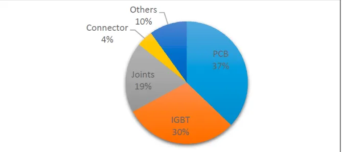
Power converters are important components of wind power plants which are responsible for different tasks such as controlling voltage and guaranteeing maximum power point tracking (MPPT). Any failure in them can affect delivery of the generated power to grid considerably. Vibration, humidity, and temperature are three main reasons that can affect the capacitor, PCB, and IGBTs performance (Peyghami, Blaabjerg & Palensky, 2020), (Luo et al., 2019).
It can be seen from Fig. 2.2 that most of failures are related to PCBs and IGBTs (Qiao & Lu, 2015).
2.1.5 Electric Machine
One of the most important components of wind power plants are electric machines which can be considered as the heart of power production in wind farms. Considering the fact that generator deals with both mechanical and electrical sections of system (responsible to transform mechanical energy to electrical one), both mechanical and electrical failures can affect its proper performance. Short-circuit, imbalance voltage and current phases are some of
Figure 2.2 Common failure rate in power converters of wind power plants Taken from Qiao et al. (2015, p. 6546)
the main electrical faults in the generators; on the other hand, air gap eccentricity, shaft, and bearing failures are among the most common mechanical failures in the generator (Yucai & Yonggang, 2016), (Artigao et al., 2020), (Zhang et al., 2020). Different tests and detection techniques are used in the literature to diagnosis these faults such as shaft displacement detection, vibration analysis, temperature monitoring, and torque measurement (Qiao & Lu, 2015).
2.2 Spectral Analysis
Another important fault diagnosis technique in generators is performing spectral analysis for electrical parameters. In (Artigao, Honrubia-escribano & Gomez-lazaro, 2018), Artigao suggests that the healthy and faulty operation conditions have their own specific signature in the spectral analysis of electrical parameters. This paper proposes the current spectral analysis for doubly-fed induction generators (DFIGs) for the first time. It is worth mentioning that the advantage of this method is that most of the failures’ frequencies are known and based on the current spectrum, the failures and root causes can be detected.
As an example, when the rotor bars break, it is known for a long time that it affects the magnetic and electrical symmetrical structure of rotor; hence, it produces a frequency component in stator current spectrum at the following frequency:
𝑓 = 𝑓 ± 2𝑠𝑓 (2.1)
Where 𝑠 is the slip and 𝑓 is the supplying frequency of generator.
Another possible failure in the generators is inter-turn short circuit in the stator winding which produces a frequency component at the following frequency:
𝑓 = 𝑓 [𝑘(1 − 𝑠 𝑝 ) ± 𝑛]
(2.2)
The unbalance rotor is another failures root cause in generators which produces stator current harmonics and can be detected via produced frequency component at the following frequency:
𝑓 = 𝑓 𝑘
𝑝(1 − 𝑠) ± 𝑙
(2.3)
Where 𝑙 is the supplying time harmonic constant.
This paper also provides other frequency components for various failures such as bearing damage, and air gap eccentricity which can be referred to detect malfunction or underperformance in the generator. The authors gathered their database from a wind farm in Spain for one year (starting September 2015) and extracted the stator current spectrum in different loading condition and also, in both super-synchronous and sub-synchronous speeds. In Fig 2.3., the stator current spectrum is shown by using FFT analysis (Artigao et al., 2018).
As it is demonstrated in Fig 2.3, there are several peak values for current in higher frequencies that might be the sign of failures. The mentioned equations can be used to check the root cause of possible failure and afterwards, rescheduling the maintenance observations.
Figure 2.3 The stator current spectrum Taken from Artigao et al. (2018, p. 5)
In (Sarma et al., 2019), Zappala developed the current spectral idea by adding stator active power and rotational speed to the studies for spectral condition monitoring. However, it should be mentioned that this paper is only about generator’s rotor electrical failure.
Table 2.1Carrier frequencies (CF) and their side-bands
Generator Signal Closed-Form Analytical Expressions
Balanced Rotor (CF) Unbalanced Rotor (𝑪𝑭 ± 𝟐𝒏𝒔𝒇)
Stator Current, Is |𝑖 ± 6𝑘(1 − 𝑠)|𝑓 |(𝑖 ± 2𝑛𝑠) ± 6𝑘(1 − 𝑠)|𝑓
Stator Active Power, Rotational Speed, Pe & Ns
|(𝑙 ± 𝑖) ± 6𝑘(1 − 𝑠)|𝑓 |((𝑙 ± 𝑖) ± 2𝑛𝑠) ± 6𝑘(1 − 𝑠)|𝑓
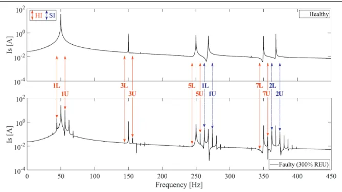
Table 2.1. indicates the possible increase in current, active power, and rotational speed spectrums due to unbalanced rotor structure. The effect on the mentioned spectrums will be as side bands (2nsf). The paper used a DFIG laboratory model with an emulated design and operational data as a DFIG harmonic model to demonstrate the proper performance of suggested frequency carriers. In the following figures, the predicted stator current and active power are shown in both healthy and unbalanced rotor condition in laboratory environment.
Figure 2.5 The stator current spectrum in different operational condition Taken from Sarma et al. (2019, p. 14)
Figure 2.4 The spectrum of active power in different operation condition Taken from Sarma et al. (2019, p. 14)
It can be seen from Fig. 2.4 and Fig. 2.5 that the anticipated carrier frequencies for current and active power are correct and side bands appeared in rotor failure condition (Sarma et al., 2019). There are still other components in wind power plants which their failure affects proper performance of the system; however, since the main failures are discussed here, the failures of other components can be neglected. The gathered data by SCADA system can be exploited for condition monitoring purposes via three different approaches: 1) Signal trending, 2) Physical models, and 3) ML and signal processing techniques.
2.3 Signal Trending
This method of analyzing SCADA data is based on comparing the measurements from one turbine with other turbines. As an example, the bearing temperature in one turbine can be compared with other bearings temperatures in other turbines and any deviations will be a sign of failure in this method. One of the techniques that are used in this method is normalizing the quantity of measured parameter in order to make the comparison easier (Orleans, 2013). As an example, the temperature of drive train in a wind farm has been demonstrated in Fig. 2.6.
Figure 2.6 Drive train temperature Taken from Orleans (2013, p. 382)
As it has been shown in Fig. 2.6, the drive train temperature of one turbine is compared with other ones in order to check the deviation. It can be seen after December 2010 the temperature deviates from expected value which can be a sign of failures. It is worth mentioning that this method is based on comparison of different turbines without considering the location of turbines and topology of wind farm. The altitude of turbines from sea level is highly affects the wind speed; hence, this method will have a high rate of false failure alarms though it might lead to detection of some failures in the system.
2.4 Physical Model
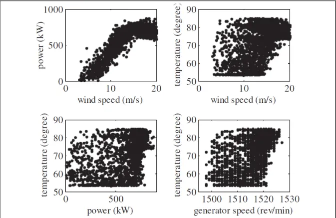
The other approach in condition monitoring of wind power plants are based on the physical and mathematical modeling of the system. In (Yang, Court & Jiang, 2013), Yang tried to refine to the data at the first step by sectionalizing the database and showing each section with only
Figure 2.7 The gathered raw data by SCADA system for 750 kW wind turbine Taken from Yang et al. (2013, p. 365)
one value. In Fig. 2.7., it has been shown how the gathered raw data for a 750-kW wind turbine are pre-processed by sectionalizing.
In Fig. 2.8., the refined data based on sectionalizing method are shown (Yang et al., 2013).
In this paper, a correlation test is also exerted to estimate the future values of parameters based on the variations in other parameters. The following equation the value of estimated value based on the correlation with other parameters.
𝑦 = 𝑎 + 𝑎 𝑥 + 𝑎 𝑥 + ⋯ + 𝑎 𝑥 (2.4)
Which the ai parameters are calculated in the sensitivity analysis of other parameters as
follows: ⎩ ⎪ ⎨ ⎪ ⎧ ( )= 0 ( ) = 0 ⋮ ( )= 0 (2.5) Figure 2.8 Pre-processed data for a 750-kW wind turbine
Where:
𝑅 = [𝑦 − 𝑦 ] (2.6)
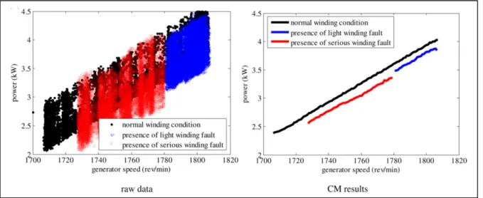
This paper uses these equations to estimate the parameters and predict the system behaviors. A 30-kW wound rotor induction generator is used in laboratory to test the proper performance of this method. The system is tested in presence of slight and severe winding failures. The pre-processing algorithm is employed on the model and the figures have been extracted as follows (Yang et al., 2013):
It can be seen that pre-processing method made the interpretation easier and also, deviations are clearer.
2.5 ML and signal processing techniques
The gathered data by SCADA system can be interpreted by using different signal processing methods. The Hilbert transform can be used for both time and frequency analysis and demodulate the target signal for feature extraction in order to make the data ready for fault
Figure 2.9 Generator winding fault detection Taken from Yang et al. (2013, p. 365)
diagnosis based on the faults’ features (Lu et al., 2013), (Gong, Qiao & Member, 2015), (Deng et al., 2019). The other signal processing method is Envelope method which is mainly used for vibration signals and detects the bearing inner and outer faults; however, it needs other signal processing methods to complete condition monitoring procedure, because this analysis is only in time domain (Weller, 2009), (Halpin et al., 2008).
The Statistical Analysis is another well-established method for fault detection wind power plants. In this method, the statistical parameters (mean value and variance) of signal is calculated and extracted for a healthy operation period and it will be recalculated for other periods. If the measured and calculated value deviate from the stored valued, it can be sign of failures in the system. It should be noted that in this method, only the occurrence of faults can be detected and prediction is not available and moreover, presence of noise in the data can highly affect to the interpretation of analysis and lead to a false alarm (Kusiak & Verma, 2012). The signals also can be divided into several different components with their specific scale and frequencies by Wavelet method to provide more data about the operation of system. The wavelet method has been used for monitoring bearings of generator and also gearbox, so far (Zimroz et al., 2012), (Watson et al., 2010), (Gray & Watson, 2010).
Using artificial intelligence is getting wide-spread in the last decade for engineering application due to enhances in computational systems. DL models are widely used in literature for anomaly detection in different systems. Here, we only focus on developed models for time-series data since the purpose of this project is to monitor temperature of generator windings provided by SCADA system with 10-min interval sampling. To handle the sequential data monitoring, Recurrent Neural Networks (RNNs) are the best choice among other developed DL topologies.
Among different RNN models, LSTM shows unique performance for analyzing time-series data with inherent dependencies to previous states of the system (Zhang, Li, Long & Ling, 2018), (Hu & Chen, 2018). In (Lei, Liu & Jiang, 2019), a classification approach is followed using LSTM for anomaly detection in wind farms by setting rotor-related signals. Moreover,
LSTM is used to predict the generated power of a wind farm for enhancing the competitiveness of wind farm in electricity market (Shi et al., 2018). However, usage of LSTMs for monitoring the generator winding is not reported in the literature. The contribution of this project is to utilize LSTM model for anomaly detection in windings of generators in wind farms.
CHAPTER 3
PROPOSED DATA PREPROCESSING TECHNIQUE And REGRESSION MODEL 3.1 Correlation Analysis
In this project, the main object is to predict the temperature of windings of generators in wind farms. For this purpose, considerable datasets of different mechanical and electrical signals are needed to be set as the inputs of ML models. Although these datasets are provided by Power Factors, several preprocessing techniques should be imposed on these raw datasets to be prepared for the models.
To increase the computation speed and decrease the complexity of model, it is crucial to decrease number of inputs to the models. The correlation analysis will be exploited in this project to determine the highly correlated features. The correlation between two datasets can be calculated as follows (Thompson , 2005):
𝑟 = ∑(𝑥 − 𝑥̅)(𝑦 − 𝑦)
∑(𝑥 − 𝑥̅) ∑(𝑦 − 𝑦) (3.1)
Where 𝑋, 𝑦 are the mean values of datasets.
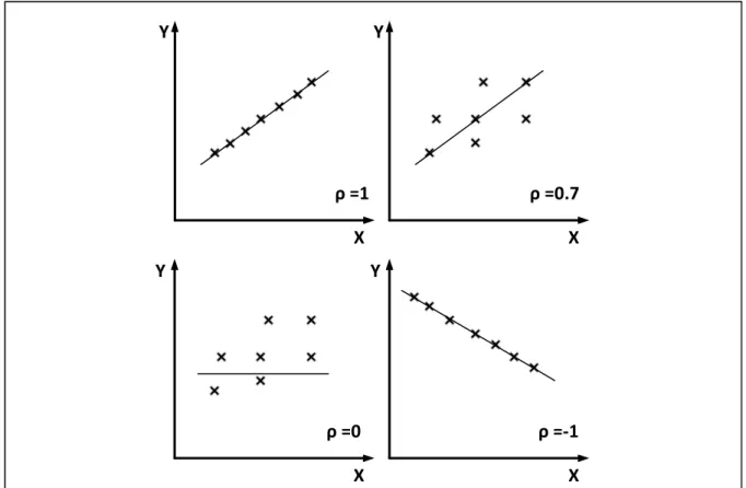
A perfect positive correlation shows that the datasets are highly and linearly correlated and follow the same variation patterns and zero correlation value means that datasets have the least possible relation between each other. Finally, negative correlation value shows that datasets are linearly but negatively related to each other.
Figure 3.1 Correlation scenarios between two variables
When two variable has a high correlation value, it can be interpreted that their trends of variation are roughly the same. Hence, one of these highly correlated variables can represent other ones and decrease the number of features and complexity of model.
3.2 Multiple Linear Regression (MLR)
A regression approach is used for modeling relationship between a dependent variable and one (Simple Linear Regression) or several independent variables (MLR). MLRs show excellent performance for predicting a target value when variables are linearly related though there will be some inevitable errors. In MLR, linear relationship between features and dependent variable is obtained as follows (Breiman & Friedman, 1997):
𝑦 = 𝑋𝛽 + 𝜀 (3.2) X Y ρ =1 X Y ρ =0.7 X Y ρ =0 X Y ρ =-1
Where: 𝑦 = 𝑦 𝑦 ⋮ 𝑦 , 𝑋 = 1⋮ 1 𝑥 … 𝑥 ⋮ ⋱ ⋮ 𝑥 … 𝑥 ; 𝛽 = 𝛽 𝛽 ⋮ 𝛽 ; 𝜀 = 𝜀 𝜀 ⋮ 𝜀
Where 𝑦, 𝑋, 𝛽, and 𝜀 are dependent variable, input features, regression coefficients, and error term, respectively. The whole MLR idea relies on the fact that there should be a linear relation between input features and output. The best linear regression is achievable by minimizing the error term in (3.2). The popular approach for minimizing the error term is mostly based on least square modeling which tries to minimize error square which is represented as follows:
𝑆(𝛽) = 𝜀 = 𝜀 𝜀 = (𝑦 − 𝑋𝛽) (𝑦 − 𝑋𝛽) (3.3)
The expanded version (3.3) is shown as follows:
𝑆(𝛽) = 𝑦 𝑦 − 𝛽 𝑋 𝑦 − 𝑦 𝑋𝛽 + 𝛽 𝑋 𝑋𝛽
= 𝑦 𝑦 − 2𝛽 𝑋 𝑦 + 𝛽 𝑋 𝑋𝛽 (3.4)
To obtain the optimal regression coefficient, the first derivative of least square equation in (3.4) is calculated as follows:
𝛿𝑆
𝛿𝛽 = −2𝑋 𝑦 + 2𝑋 𝑋𝛽 = 0 (3.5)
Hence, the optimal regression coefficient is obtained as follows:
3.3 Artificial Neural Network (ANN)
The brain functionality of humans in obtaining and processing the input signals from environmental experiences of body inspired scholars (McCulloch & Pitts, 1943) to develop an algorithm, named ANN. The developments in neural network modeling is pursed by scientists for reaching a better understanding of brain functionality and more importantly, developing algorithms and computers which have better performance in poorly defined problems such as pattern recognition and Natural Language Processing (NLP). The recent advances in computational systems made ANN-based systems the perfect choice for many different practical applications such as prediction, classification, image processing, and etc. One of the basic and widely popular types of ANNs is multi-layer perception (MLP) which shows a powerful performance in many practical aspects. The MLP structure is consists of three layers: input layer, hidden layer, and output layer. The schematic of a fully inter-connected MLP is shown in Fig. 3.2.
It is worth mentioning that the neurons are the main components of MLP layer which determine the overall performance of system. To have a better understanding about MLP’s performance, it is crucial to know exactly how a neuron or node processes the input data. The schematic of a node is presented in Fig. 3.3.
The input data from input layer are fed to neurons in the hidden layer. Each neuron assigns a weight for the incoming data from previous layer to indicate the relative importance of them. In a neuron, the propagation function is exerted to the inputs by calculating the weighted sum of inputs which is added to a bias term. The obtained propagated values of neuron are fed to activation function and the results are passed to the next layer. This structure which relies on one-way flow of information is the basic topology for neural networks which is called feed-forward neural networks.
3.3.1 Activation Function
In terms of biological neural network, the activation function acts as the rate of action potential of firing of cells. Since the activation functions play a cardinal role in obtaining a proper output, dozens of activation functions are developed, which each of them has unique performance for specific problems. Considering the studied problem in this thesis, we only focus on the most relevant activation functions.
3.3.1.1 Binary Step Function
This activation function checks the calculated weighted sum of inputs with a threshold. Once the threshold is passed the neuron is activated and sends the exact same value to the next layer. The graphical representation of Binary Step Function is shown in Fig. 3.4.
3.3.1.2 Linear Activation Function
The Linear Activation Function produces a proportional of input value and sends it to the next neuron. This activation function provides more freedom by producing multiple outputs instead of binary ones. In gradient descent algorithm, it is essential to have a relation between inputs and the derivative term of activation function and Linear Activation Function derivative term is constant and not related to the inputs; hence, the weights cannot be updated to minimize the error which makes this activation function practically useless. The Linear Activation Function is plotted in Fig. 3.5.
Figure 3.4 Binary step activation function representation
3.3.1.3 Sigmoid Function
The Sigmoid Function is a nonlinear activation function which its outputs are between 0 and 1. The Sigmoid curve in shown in Fig. 3.6.
The limitation of output between 0 and 1 means that the rate of action potential firing in the cells cannot be faster than a certain rate. The mathematical representation of sigmoid function is shown as follows:
𝜎(𝑧) = 1
1 + 𝑒 (3.7)
This activation function guarantees that the output will remain between 0 and 1. Sigmoid function provides a fixed output range with continuously differentiable spectrum for different 𝑧 values. It provides a smooth gradient which prevents any jumps in the outputs of neurons. One of the main disadvantages of this activation function is that it only produces positive output and cannot provide a proper response for problems that need negative output to reduce a variable or forget irrelevant data. Moreover, this activation function suffers from vanishing gradient problem which occurs for very high and very low values of input features. The network refuses to learn or learn very slowly in these ranges due to almost no change in the output of Sigmoid Function in these areas. However, Sigmoid Functions are widely exploited
for regression and classification problems due to their ability in providing a probability range for the output.
3.3.1.4 Hyperbolic Tangent Function
A modified version of sigmoid function is developed to produce both positive and negative output values. The output values for this activation function varies between -1 and 1. The Tanh function is plotted in Fig. 3.7.
The mathematical representation of Tanh activation function is represented as follows:
tanh(𝑧) = 2
1 + 𝑒 (3.8)
It is worth mentioning that one of the reasons for both sigmoid and Tanh activation functions popularity is their simple derivative forms which makes the backpropagation process for updating weights easier. Besides the sigmoid and Tanh functions difference in producing the negative outputs, Tanh function has a steeper gradient than sigmoid function which should be taken into account based on the problem requirements.
3.3.2 Optimizer
The main focus of an ANN is to minimize the predefined loss function in order to enhance results accuracy. Since it is impossible to calculate the perfect weights in an ANN, finding the acceptable weights is similar to an optimization problem with an algorithm of searching for the optimal weights. The most common algorithm which is used for ANNs is stochastic gradient descent (SGD) that is fortified with backpropagation of error algorithm to update the weights of ANNs. SGD tries to minimize the error by calculating the gradient of dataset and updating the weights values in direction opposite to the gradients in order to find a local minimum value. It is worth mentioning that Gradient Descent (GD) method is uses the same strategy for updating the weights and performs only one update; however, SGD updates the values for each training parameter. Hence, GD is much faster method with less precision and SGD can provide better results.
The other popular optimizer which is widely used for ML and DL problems is Adaptive Moment Estimation (Adam) which adapts the learning rate for each weight. Adam relies on the first moment of gradient, which is the mean value, and average of the second moment of gradient, which is the uncentered variance, for adapting the learning rate (Kingma & Ba, 2015). They showed that Adam considerably has lower training cost than other existing popular optimizers for a MLP algorithm on MNIST images dataset. The training costs over iterations for this problem are shown in Fig. 3.8 (Kingma & Ba, 2015).
It can be understood that Adam has the best performance in terms of training costs among the most popular optimizers. Hence, Adam optimizer is chosen in this thesis to update the weights due its considerable advantages over other existing optimizers.
3.3.3 Loss Function
The obvious definition of loss in ML models is the difference between predicted or obtained output values and the target variables. However, the main challenge is choosing the best method for obtaining the mentioned difference. One of the most popular loss functions for ANNs is Mean Square Error (MSE) which is the average of squared difference between predicted values and target ones. The predictions which are very far away from actual values have considerable effect on MSE value due to squaring. The mathematical representation of MSE is written as follows:
Figure 3.8 Training cost of MNIST MLP with dropout Taken from Kingma et al. (2015)
𝑀𝑆𝐸 = ∑ (𝑦 − 𝑦 )
𝑛 (3.9)
Another equally popular loss function for ML models is Mean Absolute Error (MAE) which is average of sum of errors between predicted and actual target variables. This criterion, same as MSE, neglects the direction of errors by using absolute values of error. However, implementation of MAE is harder than MSE for computing the gradients. On the other hand, MAE has a better performance with outliers since it does not use squared values of error. The MAE concept is formulated as follows:
𝑀𝐴𝐸 =∑ |𝑦 − 𝑦 |
𝑛 (3.10)
Mean Bias Error (MBE) is another less popular loss function which is used in ML applications. Considering the direction of error and positive or negative bias is the only merit of this loss function over MAE and MSE.
𝑀𝐵𝐸 = ∑ (𝑦 − 𝑦 )
𝑛 (3.11)
Cross Entropy is a well-known loss function which is widely used for classification problems. This loss function utilizes a logarithmic equation of predicted variables to offer a probability value for the output. The deviations of predicted values from the actual ones will increase the Cross Entropy. The mathematical representation of Cross Entropy is written as follows:
𝐶𝑟𝑜𝑠𝑠𝐸𝑛𝑡𝑟𝑜𝑝𝑦𝐿𝑜𝑠𝑠 = −(𝑦 log(𝑦 ) + (1 − 𝑦 )log (1 − 𝑦 )) (3.12)
It is obvious from (3.12) that when 𝑦 = 1 the second term will disappear and 𝑦 = 0 will eliminate the first term of equation.
3.3.4 Learning Rate
The step size which indicates the speed and precision of optimizer is called learning rate of neural network. It is crucial to assign a proper learning rate for finding the minimum in order to update the weights of neural network. A high learning rate can lead to neglecting the minimum point in the optimization surface while a low learning rate slows the searching operation or get stuck the operation in a local minimum. The graphical representation of this challenge is shown in Fig. 3.9.
3.3.5 Dropout
The whole concept of learning for a model relies on splitting dataset to training and testing section. The training dataset usually have higher portion of the whole dataset. Training process is exerted by feeding the training datasets to the model in order to find a relation between the target values and training data. Once the model established a reliable relation between them, the testing dataset will be fed to model in order to check the performance of model. Implementation of a precise training model relies on many factors such as the portion of training data to whole dataset, selected input features, the applied filtering range on training data, number of hidden layers, number of neurons, optimizer algorithm, batch size, loss function, number of epochs, time steps, and etc.
Proper adjustment of these parameters, which are called hyperparameters, can vastly increase the efficiency and precision of training process; however, some models will still be highly dependent to the training datasets and perform poorly on any new dataset such as testing data. This phenomenon is called overfitting or overtraining which considerably make the model unreliable. The overfitting problem intensifies when the number of hidden layer increases; hence, DL models usually suffer from overfitting. To overcome this challenge, dropout strategy is widely used by developers.
Dropout strategy, which is a regularization process, randomly ignores the outputs of some neurons in a layer (Hinton et al., 2012). Since this process is random, different neurons of a layer are ignored in each iteration. The graphical representation of dropout is presented in Fig. 3.10.
Although this process makes the network performance noisy, it diminishes the adaptation of neurons to the input dataset. Dropout can be applied to input or hidden layers but not the output layer. Implementation of dropout on a network creates a new hyperparameter which can be tuned for achieving highest precision without overfitting. It should be noted that the weights will be larger in a network with dropout strategy since some of the neurons stopped working; hence, it is crucial to scale the weights based on the dropout rate of each layer (Srivastava et al., 2013).
3.4 Recurrent Neural Network (RNN)
RNN is the developed form of ANNs which can perfectly handle time-series and sequential datasets for applications such as machine translation, stock market prediction, text generations and etc. ANNs are usually used for datasets that are independent from each other while RNNs are specifically designed to work with datasets that are dependent to each other (Zaremba, Sutskever & Vinyals, 2014). In RNNs, ANN’s backbone is added by a cell memory to look back on a few steps for predicting the future values. The representation of RNN is shown in Fig. 3.11.
Where 𝑊 , 𝑊 , 𝑥, ℎ, and 𝑐 vectors are the past information weights, input weights, input features, prediction vector, and past information of system, respectively. Fig. 3.11. shows unfolded RNN which means that the neural networks are extended over the chosen sequence. As an example, if the studied problem is Machine Translation and chosen sequence contains 5 words, it means that RNN is unfolded over 5 hidden layers which each layer represents one word. The memory state at time step 𝑡 is related to the inputs of RNN and previous states of network. RNNs show an acceptable performance for applications where the gap between relevant information and current time is narrow. In the other word, RNNs performance decreases where the gap between previous states and current time step is very wide.
3.4.1 Vanishing Gradient Challenge:
After obtaining ℎ(𝑘), the prediction error vector at time step 𝑘, 𝐸(𝑘), is calculated. These error values are used for calculating the gradients in Back Propagation Through Time algorithm which is formulated as follows (Hochreiter, 1998):
𝜕𝐸 𝜕𝑊 =
𝜕𝐸
𝜕𝑊 (3.13)
Due to simplicity, the basic GD algorithm is considered for learning process. The gradient of errors on 𝑘 time-step is calculated as follows:
𝜕𝐸 𝜕𝑊 = 𝜕𝐸 𝜕ℎ 𝜕ℎ 𝜕𝑐 … 𝜕𝑐 𝜕𝑐 𝜕𝑐 𝜕𝑊 = 𝜕𝐸 𝜕ℎ 𝜕ℎ 𝜕𝑐 ( 𝜕𝑐 𝜕𝑐 ) 𝜕𝑐 𝜕𝑊 (3.14)
The 𝑊 vector represents the weights of RNN and it is used to calculate 𝑐 as follows:
𝑐 = 𝜎(𝑊 𝑐 + 𝑊 𝑥 ) (3.15)
By calculating the derivative of 𝑐 and replacing it in (3.14), the backpropagation gradient can be obtained as follows: 𝜕𝐸 𝜕𝑊 = 𝜕𝐸 𝜕ℎ 𝜕ℎ 𝜕𝑐 ( 𝑡𝑎𝑛ℎ (𝑊 𝑐 + 𝑊 𝑥 )𝑊 ) 𝜕𝑐 𝜕𝑊 (3.16)
Larger 𝑘 can vanish the second term value in (3.16) since the tanh activation function derivative value is smaller than 1. Moreover, the multiplication of derivatives term can explode when the 𝑊 is large enough to prevail the tanh small derivative effect. This process is called exploding gradients. The main problem of RNNs is vanishing gradients challenge which can
stop the learning process of network. The mathematical representation of vanishing gradients is shown as follows: [ 𝜎 𝑊 𝑐 + 𝑊 𝑥 )𝑊 → 0 ≡ 𝜕𝐸 𝜕𝑊= 𝜕𝐸 𝜕𝑊→ 0 ≡ 𝑊 ← 𝑊 − 𝛼 𝜕𝐸 𝜕𝑊 ≈ 𝑊 (3.17)
Hence, the networks weights update will stop and no reasonable learning will occur over time.
3.5 Long-Short Term Memory (LSTM)
As it was mentioned earlier, RNNs are widely used for analyzing time-series datasets. RNNs are enhanced version of multilayer neural networks which can consider previous states of system in predicting current or future states. This will act as a memory-based model that will be a suitable choice for sequential datasets. The simple structure of LSTM is shown in Fig. 3.12.
Figure 3.12 Simple LSTM structure
LSTM Cell LSTM Cell LSTM Cell
C
t-1h
t-1X
tC
th
tX
t-1X
t+1C
t+1h
t+1C
t-2h
t-2After developing RNNs, LSTMs are introduced specifically to handle datasets that have long-term dependencies. The LSTM structure consists of input, forget, and output gates and memory cell which is illustrated in Fig. 3.13.
Figure 3.13 LSTM structure
The memory cell in each time step is responsible for deciding the eligible information for storing. The new information and previous output from last unit is fed to LSTM unit to pass from tanh layer and a sigmoid function layer to indicate which information should or should not be stored. Note that like other neural network the inputs should be scaled because sigmoid functions are operating between 0 and 1.
The forget layer consists of a sigmoid function and the information which is stored from previous LSMT units. The sigmoid function illustrates which information should be remembered for the next units. At the end, the output layer uses a tanh function to determine the information needed to pass to the output and next unit of LSTM. The mathematical equations of LSTM are elaborated in the following:
𝑓 = 𝜎(𝑊 𝑥 + 𝑈 ℎ + 𝑏 ) (3.18)
sigmoid
tanh
sigmoid
sigmoid
tanh
Forget Gate
Input Gate Output Gate
Cell State Update
C
t-1C
tf
ti
tC
t’O
th
th
t-1X
t𝑖 = 𝜎(𝑊 𝑥 + 𝑈 ℎ + 𝑏 ) (3.19)
𝑜 = 𝜎(𝑊 𝑥 + 𝑈 ℎ + 𝑏 ) (3.20)
𝑐 = 𝑓 ⨀𝑐 + 𝑖 ⨀tanh (𝑊 𝑥 + 𝑈 ℎ + 𝑏 ) (3.21)
ℎ = 𝑜 ⨀tanh (𝑐 ) (3.22)
𝑜 = 𝑓(𝑊 ℎ + 𝑏 ) (3.23)
Where 𝑏 is bias and 𝑥 and ℎ are input and hidden vectors, respectively. In addition, 𝑊 and 𝑈 are input to hidden and hidden to hidden weights matrices, respectively.
As it was mentioned earlier, RNNs suffer from vanishing gradients while LSTMs show excellent performance in handling this challenge. To calculate the gradients of error for LSTMs, we should obtain the derivative of cell state gradient which is a key term in (3.14). The derivative of LSTM cell state is calculated as follows (Hochreiter, 1998):
𝜕𝑐 𝜕𝑐 = 𝜕 𝜕𝑐 [𝑐 ⨂𝑓 ⊕ 𝑐̃ ⨂𝑖 ] = 𝜕 𝜕𝑐 [𝑐 ⨂𝑓 ] + 𝜕 𝜕𝑐 [𝑐̃ ⨂𝑖 ] = 𝜕 𝜕𝑐 𝑐 + 𝜕𝑓 𝜕𝑐 𝑐 + 𝜕𝑖 𝜕𝑐 𝑐̃ + 𝜕𝑐̃ 𝜕𝑐 𝑖 (3.24)
Where each term can be calculates as follows:
𝜕𝑓 𝜕𝑐 𝑐 = 𝜕 𝜕𝑐 𝜎(𝑊 [ℎ , 𝑥 ]) 𝑐 = 𝜎 (𝑊 [ℎ , 𝑥 ])𝑊 𝜕ℎ 𝜕𝑐 𝑐 = 𝜎 (𝑊 [ℎ , 𝑥 ])𝑊 𝑜 ⨂𝑡𝑎𝑛ℎ (𝑐 )𝑐 (3.25)