A mountain pass for reacting molecules

A Mountain Pass for Reacting Molecules

CEREMADE, CNRS UMR 7534, Universit´e Paris IX Dauphine, Place du Mar´echal de Lattre de Tassigny, 75775 Paris Cedex 16, France

E-mail: lewin@ceremade.dauphine.fr

Abstract

In this paper, we consider a neutral molecule that possesses two distinct stable positions for its nuclei, and look for a mountain pass point between the two minima in the non-relativistic Schr¨odinger framework.

We first prove some properties concerning the spectrum and the eigen-states of a molecule that splits into pieces, a behaviour which is observed when the Palais-Smale sequences obtained by the mountain pass method are not compact. This enables us to identify precisely the possible values of the mountain pass energy and the associated ”critical points at infinity” (a concept introduced by Bahri [2]) in this non-compact case.

We then restrict our study to a simplified (but still relevant) model: a molecule made of two interacting parts, the geometry of each part being frozen. We show that this lack of compactness is impossible under some natural assumptions about the configurations ”at infinity”, proving the existence of the mountain pass in these cases. More precisely, we suppose either that the molecules at infinity are charged, or that they are neutral but with dipoles at their ground state.

AMS Subject Classification: 35B38, 35Q40, 35J10, 49J35, 81V70, 81V55, 81Q05, 49S05.

Keywords: mountain pass, critical points, critical points at infinity, Morse index, quantum mechanics, ground state, excited state, quantum chemistry, reaction path, transition state.

Introduction

In this paper, we study in the non-relativistic quantum Schr¨odinger framework the case of a molecule that possesses two distinct stable positions for its nuclei, as this is for instance the case for HCN and CNH. Our purpose is somewhat simple: can we obtain a critical point of the energy by using the classical moun-tain pass method between the two minima ? Experiment suggests that this is the case (at least for the HCN↔CNH reaction). Indeed, such mountain pass points are frequently computed by chemists who need to understand the possi-ble behaviour of the molecule: it corresponds to a ”transition state” during an infinitely slow reaction leading from one minimum to the other. But as far as we know, this problem has never been tackled from the mathematical point of view for the N -body quantum problem, or even in the context of the classical Hartree or Thomas-Fermi type models which are approximations of the exact theory.

For a neutral molecule, the proof that there is a minimum with regards to the position of the nuclei can be found in the fundamental work of E.H. Lieb and W. E. Thirring [25] for the Schr¨odinger model, and in a series of papers by I. Catto and P.-L. Lions [4, 5, 6, 7] for approximate models (Hartree or Thomas-Fermi type), the latter being really more complicated due to the non linearity of these models. In these two works, the authors had to prove that minimizing sequences are compact, the non-compactness behaviour being related to the fact that the molecule can split into parts, each moving away from the others. Remark that binding does not occur for the Thomas-Fermi model (see the works of E. Teller [31], E.H. Lieb and B. Simon [24], and the references in [4]) and that the result is not known for the Hartree-Fock model, except in very special cases [7].

Let us make some comment on a tool used in these proofs that cannot be simply adapted to our setting. A common idea in these two works is to average over all the possible orientations of each piece in order to simplify the computation of the interaction energy between them, by suppressing the multipoles. To show that the energy can be lower than the energy at infinity, a new term using the correlation between the electrons is then created in [25] to obtain a Van Der Waals term of the form −C/R6 _{(R is the distance between}

the molecules), while a very detailed computation of the (exponentially small) combined energy is done in [4, 5, 6, 7] to conclude that the system can bind. Because of the preliminary averaging, the conclusion is that there exists some orientation of the molecules for which this is true, but this position is unknown a priori.

In the case of the mountain pass method that we propose here, the non-compactness is obviously also due to a possible splitting of the molecule. How-ever, we want to insist on the fact that we cannot use in this setting the same idea of averaging over all the rotations of the molecules, because we have to pull down the energy along a path. In other words, a comparison between the energies is not sufficient to conclude, and a precise information on the directions on which the energy decreases is needed.

This is why we failed to treat the problem in its full generality and we had to add some hypothesis about the configurations ”at infinity”. Nevertheless, we wish to ameliorate this first work in the future, and hope that it will stimulate further results.

The results proved in this paper are the following.

First, we study the spectrum and the eigenfunctions of the Hamiltonian when a molecule splits into parts. We obtain some bounds on the eigenvalues and the bottom of the essential spectrum which allow to show that the ”elec-trons remain in the vicinity of the nuclei” when a fixed excited state is studied. In other words, no electron is lost during the process. This is obtained by a non-isotropic exponential decay of the electronic density, which is shown to be uniform when the distance between the molecules grows. We also specify the behaviour of the associated wavefunctions and define the ”critical points at in-finity”, a concept introduced by A. Bahri [2]. Some parts of this first result are necessary for our min-max problem.

Then, we prove a result that enables to identify the possible behaviour of the non-compact min-maxing paths. As it is suggested by the intuition, it is shown that the optimal energy of the mountain pass corresponds in this case to a system where the molecule is split into independent parts (the electrons are shared among them), each being at its ground state. This Morse information on the critical points at infinity is rather intuitive.

As announced, we were unable to treat the general case and we end this article by showing that this non-compactness behaviour is impossible in the special case of two interacting molecules with fixed nuclei. This is done under the hypothesis that we are in the easy case of two charged molecules at infin-ity, or in the more difficult case of two neutral molecules at infininfin-ity, but with dipoles at their ground state. This enables to obtain the required result for many practical situations. As explained before, the crucial step is to evaluate the interaction energy between the molecules and we use here a multipole ex-pansion, even for wavefunctions that are not a simple tensor product of two ground states as in [25]. Finally, the expected result is deduced from the fact that the critical points of the dipole/dipole interaction energy which have a nonnegative energy have a Morse index which is at least 2.

From a practical point af view, the study of this mountain pass method is really important. As mentioned above, the main idea is that a path leading from one minimum to the other represents an infinitely slow chemical reaction. The mountain pass energy is then interpreted as the lowest energy threshold for the reaction to happen. The numerical computation of this energy and of the optimum (even the whole path) is then a prime necessity for chemists, who have to understand the possible behaviours of the molecule (see for instance [28, 9] for chemical and numerical aspects).

However, chemists only consider paths on which the molecule is at its ground state all along it, which leads to obvious problems of smoothness in the case of degeneracy of the first eigenvalue of the Hamiltonian, and can obstruct con-vergence. For mathematical reasons, we were thus forced to abandon this

hy-pothesis and relax the problem by considering that the wavefunction can vary independently of the nuclear geometry, in order to obtain a critical point with respect to nuclei’s variations. Since we shall show that our min-max energy is in fact the same that the one used in practice, this approach could also be interesting for numerical computations.

We conclude with a few words on the mathematical tools used in this paper. As in [4, 5, 6, 7], the proof is guided by P.-L. Lions’ Concentration-Compactness ideas [26], although the localization of the electrons is given by the uniform exponential decay of Theorem 2, and not by this theory. Let us remark that the physical intuition is somewhat often related to the behaviour of the electronic density. For instance, when the molecule splits into parts, the latter becomes a sum of functions localized near the nuclei. But this point of view is not sufficient to understand the problem since the main object is not the density, but the wavefunction. The latter will not split into sums, but into sums of tensor products of wavefunctions in lower dimensions (see the work of G. Friesecke [10] for a very clear explanation of this phenomenon). Therefore, we use a variant of N -body geometric methods for Schr¨odinger operators [30, 29, 18] that enables to relate the behaviour of the wavefunction to those of the associated electronic density. This method is used in [10] and enabled G. Friesecke to notice an interesting link between the celebrated HVZ Theorem [18, 32, 33] and the Concentration-Compactness method [26].

Moreover, the HVZ Theorem (which enables to identify the bottom of the spectrum as the ground state energy of the same system but with an electron removed), and Zhislin’s Theorem (which states the existence of excited states for positive or neutral molecules) are abundantly used in this article.

Finally, we use the results and methods developed by G. Fang and N. Ghous-soub [8, 14] which enable to obtain Morse information on the Palais-Smale sequences, related to the fact that the deformed object are paths (i.e. deforma-tions of [0; 1]). We also use the duality theory developed in [14] which permits to locate critical points.

The paper is organized as follows. In the next section, we describe the model in detail and recall known results on the Hamiltonian and its eigenfunctions. Then, in section 2, we present our results without proof: for the sake of clarity, we have brought all the proofs together in the last section.

Acknowledgments: I would like to thank ´Eric S´er´e for his constant attention and helpful remarks.

1

The model

We consider here a positive or neutral molecule with N non relativistic electrons, and M nuclei of charges Z1+ · · · + ZM ≥ N . The nuclei are supposed to be

and are thus represented as pointwise charges at R1, ..., RM ∈ R3. In what

follows, we let

R = (R1, ..., RM) ∈ Ω := (R3)M \ (∪i6=j{Ri = Rj})

and

Z = (Z1, ..., ZM) ∈ (N∗)M, |Z| = Z1+ · · · + ZM ≥ N.

The system is described by the purely coulombic N -body Hamiltonian HN(R, Z) = N X i=1 µ −1 2∆xi+ VR(xi) ¶ + X 1≤i<j≤N 1 |x_i− x_j|+ X 1≤i<j≤M ZiZj |R_i− R_j|, V_R(u) = − M X j=1 Zj |u − Rj| . Its operator domain is the Sobolev space H2

a(R3N, C), and its quadratic form

domain is H_a1(R3N, C). Throughout this paper, the subscript a indicates that we consider wavefunctions Ψ which are antisymmetric under interchanges of variables (expression of the Pauli exclusion principle):

∀σ ∈ SN, Ψ(x1, ..., xN) = ²(σ)Ψ(xσ(1), ..., xσ(N )).

The quantum energy of the system in a state Ψ ∈ H_a1(R3N, C) is the associated quadratic form

EN(R, Ψ) =­Ψ, HN(R, Z)Ψ®.

We refer the reader to [22, 3] for a description of this model and a de-tailed explanation of the Born-Oppenheimer approximation. The properties of HN_{(R, Z) and its eigenfunctions are recalled below. For the sake of}

simplic-ity, we have neglected the spin and the dynamic of the nuclei, as in [25]. We would like also to mention that all the results in this paper can be adapted to the case of smeared nuclei, that is to say when the Coulomb potential _|x−R1

i|

is replaced by R_R3 _|x−y−R1

i|dµi(y) where µi is a probability measure on R

3_{. Of}

course, _|R 1

i−Rj| has to be replaced by

RR

R6 _|Ri+y−(R1 _j+z)|dµi(y)dµj(z). Remark

that, in contrast to many other papers dealing with minimization, we work here with complex-valued wavefunctions, a hypothesis that plays a role in our results (see for instance Theorem 4 and the associated remarks).

Z and N being fixed such that N ≤ |Z|, for each R ∈ Ω, the problem EN(R, Z) = min{EN(R, Ψ), ||Ψ||_L2 = 1}

has a solution Ψ, which is the ground state of the N electrons interacting with the M nuclei localized at the Ri.

For neutral molecules (N = |Z|), it is also known that the problem EN = min

R∈ΩE

admits a solution [25], proving the stability of neutral molecules.

We shall assume that (R, Ψ) and (R0_{, Ψ}0_{) are two local minima of E}N_{. We}

then consider the classical mountain pass method c = inf γ∈Γt∈[0;1]max E N_{(γ(t)) (1)} where Γ = {γ ∈ C0([0; 1], Ω × SH_a1(R3N)), γ(0) = (R, Ψ), γ(1) = (R0, Ψ0)} SH_a1(R3N) = {Ψ ∈ H_a1(R3N), ||Ψ||_L2 = 1}

and want to show that c is a critical value of EN_.

As mentioned in the introduction, the physical interpretation of this min-max method is that paths γ ∈ Γ represent an infinitely slow reaction leading from one minimum to the other. c is thus interpreted as the lowest energy threshold for passing from (R, Ψ) to (R0_{, Ψ}0_).

In practice, the following definition is used c0 = inf

r∈Rt∈[0;1]max E

N_{(r(t), Z)}

where

R = {r ∈ C0([0; 1], Ω), r(0) = R, r(1) = R0}.

As explained in the introduction, the function R 7→ EN_{(R, Z) is continuous but}

not necessary differentiable and this is why we shall study the min-max method (1). However, it will be shown that in fact c = c0_.

1.2 Properties of HN_{(R, Z)}

Let us now recall some well-known facts about the spectrum of HN_{(R, Z). We}

introduce

λN_d(R, Z) = inf

dim(V )=d _{Ψ ∈ V,}sup ||Ψ||L2= 1

hH(R, Z)Ψ, Ψi. (2)

In the sequel, we shall denote for all d ≥ 1 E0(R, Z) = λ0_d(R, Z) := X 1≤i<j≤M ZiZj |Ri− Rj|, Σ 0_{(R, Z) = +∞.} For a wavefunction Ψ ∈ H1

a(R3, C), the electronic density and the electronic

kinetic energy density are respectively defined by ρ_Ψ(x) = N Z R3(N −1) |Ψ(x, x₂, ..., x_N)|2dx₂...dx_N t_Ψ(x) = N Z R3(N −1) |∇Ψ(x, x2, ..., xN)|2dx2...dxN.

Theorem 1. We assume N ≥ 1. The following results are known : 1. (Self-adjointness [20]) HN_{(R, Z) is self-adjoint on L}2

a(R3N) with

op-erator domain H2

a(R3N) and quadratic form domain Ha1(R3N).

2. We have [19] σess ¡ HN(R, Z)¢= [ΣN(R, Z); +∞) ∀d ≥ 1, λN_d(R, Z) ≤ ΣN(R, Z) ≤ X 1≤i<j≤M ZiZj |Ri− Rj| 3. (HVZ Theorem [18, 32, 33, 19]) We have ΣN(R, Z) = EN −1(R, Z). 4. (Compactness below the essential spectrum) If λN

d(R, Z) < ΣN(R, Z),

then λN_d(R, Z) is an eigenvalue of finite multiplicity and in particular, there exists a Ψd∈ Ha2(R3N) such that

HN(R, Z)Ψd= λNd(R, Z)Ψd.

It is locally lipschitz [21], i.e.

Ψ_d∈ C0(R3N) and |∇Ψ_d| ∈ L∞_loc(R3N),

and real analytic [13] on UN \ {xi = xj}, where U = R3\ {Ri}Mi=1. If ρd

is the associated electronic density, then [13] ρd∈ Cω(U ) ∩ C0,1(R3).

5. (Zhislin Theorem [33]) For positive and neutral molecules N ≤ |Z|, then

λN_d(R, Z) < ΣN(R, Z) for all d ≥ 1, so that

σ¡HN(R, Z)¢= {λN₁ (R, Z) ≤ · · · ≤ λN_d(R, Z) ≤ · · · } ∪ [ΣN(R, Z); +∞). 6. (Negative molecules [19, 23]) For negative molecules N > |Z|, there exists a δ such that λN_δ (R, Z) = ΣN(R, Z), and δ = 1 when N ≥ 2|Z|+M . Note that the functions ΣN_{(R, Z) and λ}N

d(R, Z) (d ≥ 1) are continuous

with respect to R.

2

The results

In this section, we present the results that we have obtained concerning the mountain pass method defined above. As mentioned, all the proofs are post-poned to the next section.

2.1 The spectrum of a molecule that splits into pieces

We begin the study by some general results about the spectrum and the be-haviour of the eigenstates when the molecule splits into pieces, that is to say when |Ri− Rj| → +∞ for some i and j. As mentioned above, this splitting

of the molecule will be shown to be the main reason for the possible lack of compactness of Palais-Smale sequences.

Although only the case of ground states will be necessary for the sequel, we tackle here arbitrary excited states. In this section, we consider a positive or neutral molecule (N ≤ |Z|). × × × × O X1 X2 X3 Z1 Z2 Z3 Z4 Z5 Z6 Y r2,1 > t * +

Figure 1: An example with M = 6, p = 3, m1 = 3, m2= 1 and m3 = 2.

We fix a 2 ≤ p ≤ M (number of pieces).

Let X1, ..., Xp : R+ 7→ R3 be p functions that satisfy |Xi(t) − Xj(t)| ≥ t

for all i 6= j and t large enough. Let be m = (m1, ..., mp) ∈ (N∗)p such

that Pp_j=1mj = M . We fix a positive constant R0 and some rj,k ∈ R3 and

zj,k ∈ N for j = 1, ..., p and k = 1, ..., mj such that |Z| :=

P_p

j=1

Pmj

k=1zj,k ≥ N ,

|r_j,k| ≤ R0 and rj,k 6= rj,l when k 6= l. We then let

zj = (zj,1, ..., zj,mj), Z = (z1, ..., zp), rj = (rj,1, ..., rj,mj), ˜ rj(t) = (Xj(t) + rj,1, ..., Xj(t) + rj,mj), R(t) = (˜r1(t), ..., ˜rp(t)). We also introduce ωj = {(rk) ∈ B(0, R0)mj, rk1 6= rk2 if k1= k2}. and U(R) = R3\   p [ j=1 B(Xj, R)   .

2.1.1 Spectrum and uniform exponential decay We have the following result:

Theorem 2 (Spectrum and uniform exponential decay). For all 1 ≤ N ≤ |Z| and all d ≥ 1, we have

1. lim t→+∞E N_{(R(t), Z) = min}    p X j=1 ENj_(r j, zj), N1+ ... + Np = N   . 2. lim sup t→+∞ λ N d(R(t), Z) ≤ min    p X j=1 λNj δj (rj, zj), N1+ ... + Np= N, p Y j=1 δj = d   . 3. inf rj∈ωj lim inf t→+∞ ¡ ΣN(R(t), Z) − λN_d(R(t), Z)¢> 0.

4. Let ΨR be an eigenfunction associated to the eigenvalue λN_d(R, Z), with

associated densities ρ_R and t_R. Then there exist positive constants R1, C

and α, depending only on N , d, R0, p such that

ρR(x) ≤ C exp(−αδ(x)) and tR(x) ≤ C exp(−αδ(x)) on U(R1)

where δ(x) = min{|x − Xj|, j = 1, ..., d}.

The first part 1) identifies the limit of the ground state energy. This type of result is rather intuitive and classical. However, since we do not know a reference in this precise setting, a proof will be given in the next section.

The interpretation of the last part 4) is that if a neutral or positively charged molecule splits into parts, then for a fixed excited state, the electrons remain in the vicinity of the nuclei.

For the sake of simplicity, let us denote, for r = (r₁, ..., r_p) and z = (z₁, ..., z_p) ΛN_d (r, z) := min    p X j=1 λNj δj (rj, zj), N1+ ... + Np = N, p Y j=1 δj = d   . 2.1.2 Behaviour of the wavefunctions, critical points at infinity

Now that we have some bounds on the eigenvalues and the bottom of the essential spectrum, we want to prove a result describing the behaviour of the eigenfunctions. This will enable us to define the ”critical points at infinity” of the model, a concept that was introduced by A. Bahri [2].

The right hand side of Theorem 2 - 1), or more generally an equality like c = p X j=1 λNj δj (rj, zj), (3)

is rather standard from P.-L. Lions’ Concentration-Compactness point of view: when the molecule splits into pieces, then the energy of an electronic excited

states becomes a sum of excited states energies of the pieces. In other words, a ”critical point at infinity” would be a system constituted by p molecules in some excited state, each being infinitely far from the others, so that the interactions between them vanish.

Let us consider a sequence t_n → +∞, some r = (r₁, ..., r_p) ∈Np_j=1ω_j, and denote by Rn_{= R(t}

n) := (X1(tn) + r1, ..., Xp(tn) + rp), Xjn = Xj(tn). For the

electronic density, such a configuration is then clearly obtained in the case of dichotomy, that is to say ρn_'Pp

j=1ρnj where ρnj is essentially supported in the

vicinity of X_jn (see the exponential decay of Theorem 2). But the behaviour of the wavefunction Ψn_{is less simple since these functions will not split into sum}

of functions, but into sums of antisymmetric tensor products of wavefunctions in lower dimensions. In other words, a simple way to represent these non interacting molecules in terms of the wavefunction is to take

Ψn= τXn

1 · ψ1∧ · · · ∧ τXpn· ψp (4)

where each ψj is an eigenfunction of HNj(rj, zj) associated to the eigenvalue

λNj

δj (rj, zj). We have used here the notation

τv· Ψ(x1, ..., xN) := Ψ(x1− v, ..., xN − v)

and we recall that the tensor product is defined for ψ ∈ L2

a(R3N1) and ψ0 ∈ L2 a(R3N2) by ψ ∧ ψ0(x1, ..., xN1+N2) = 1 √ N !N1!N2! X σ∈SN ε(σ)ψ(x1_σ)ψ0(x2_σ). where x1 σ := (xσ(1), ..., xσ(N1)) and x2σ = (xσ(N1+1), ..., xσ(N )).

With (4), one easily sees that ρn ₌ Pp

j=1τXjn · ρj with obvious notations,

and that

HN(Rn, Z)Ψn− cΨn→ 0 in L2_(R3N_{) as n → +∞.}

When a λNj

δj (rj, zj) is degenerated, we can obtain the same behaviour by

taking a wavefunction which is a sum of such antisymmetric tensor products Ψn∈ p ^ j=1 τXn j · ker ³ HNj_(r j, zj) − λN_δjj(rj, zj) ´ . To simplify notations, we shall denote τn·(ψ1∧· · ·∧ψp) := τXn

1 ·ψ1∧· · ·∧τXpn·ψp, so that Ψn= τn· Ψ where Ψ ∈ V_p j=1ker ³ HNj_(r j, zj) − λN_δjj(rj, zj) ´ .

Suppose now that a molecule splits into two identical pieces: r1 = r2 and

z₁ = z₂, and that N₁ 6= N₂. At infinity, we shall obtain two molecules with the same configurations of the nuclei, but not the same number of electrons. Since there is no reason to distinguish the two states obtained by inverting the electrons between the two molecules, a wavefunction can be a sum of these two states with the same energies. We are thus led to introduce the following definition.

Definition 1. Let rn _{= (r}n

1, ..., rnp) ∈

N_p

j=1ωj be such that rjn→ rj ∈ ωj, and

Rn_{= R(t}

n) := (X1(tn) + r1, ..., Xp(tn) + rp), Xjn= Xj(tn), for some tn→ +∞.

Let c be such that the set AN_c (r, z) =   (Nj, δj) ∈ (N p₎2_{, N} 1+ · · · + Np = N, p X j=1 λNj δj (rj, zj) = c    (5) is not empty. The sequence (Rn_{, Ψ}n_{) in Ω × SH}1

a(R3N) converges to a critical

point at infinity of energy c if there exists some

Ψ ∈ X (Nj,δj)∈ANc (r,z)   p ^ j=1 ker ³ HNj_(r j, zj) − λN_δjj(rj, zj) ´  ₍₆₎ such that ||Ψn− τn· Ψ||H1 a(R3N)→ 0. (7)

To justify the term critical point, we remark that one can prove Lemma 1. Let be c and Ψ that satisfy (5) and (6). Then

(HN(Rn, Z) − c)(τn· Ψ) → 0

in L2(R3N).

Details will be given later on.

Saying differently, a critical point at infinity is a class

τ_K(r, Ψ) =©τ_X1,...,Xp(r, Ψ), X_j ∈ R3, |X_i− X_j| ≥ Kª where Ψ ∈ P_(Nj,δj)∈AN c(r,z) ³V_p j=1ker ³ HNj_(r j, zj) − λN_δjj(rj, zj) ´´ , rj ∈ ωj

and τX1,...,Xp is defined on each Ω ×

V_p

j=1Ha1(R3Nj) by

τX1,...,Xp· r = (X1+ r1, · · · , Xp+ rp)

τ_X1,...,Xp· (ψ1∧ · · · ∧ ψp) = (τX1ψ1) ∧ · · · ∧ (τXpψp).

A sequence (Rn, Ψn) converges to this critical point at infinity when there exists a Kn→ +∞ such that

lim

n→+∞d[(R

n_{, Ψ}n_{); τ}

Kn(r, Ψ)] = 0.

Let us now fix a sequence t_n → +∞ and some rn _{= (r}n

1, ..., rpn) ∈

N_p

j=1ωj

such that rn_j → rj ∈ ωj, and denote Rn = R(tn), Xjn= Xj(tn). We then have

Theorem 3. We assume 1 ≤ N ≤ |Z| and d ≥ 1. Let (Ψn_{) be a sequence of}

wavefunctions such that

HN(Rn, Z) · Ψn= λN_d(Rn, Z) · Ψn.

Then, up to a subsequence, we have limn→+∞λN_d(Rn, Z) := c with

ΛN₁ (r, z) ≤ c = p X j=1 λNj0 δ0 j (rj, zj) ≤ Λ N d(r, z) for some (N0

j, δj0) ∈ ANc (r, z), and (Rn, Ψn) converges to a critical point at

infinity of energy c.

2.2 The mountain pass method: a general result

Let us now come back to our mountain pass method, and consider again a neutral molecule (N = |Z|). Recall that (R, Ψ) and (R0, Ψ0) are two local minima of (R, Ψ) 7→ EN_{(R, Ψ), and that c and c}0 _{are defined by}

c = inf γ∈Γt∈[0;1]max E N_{(γ(t)) (8)} Γ = {γ ∈ C0([0; 1], Ω × SH_a1(R3N)), γ(0) = (R, Ψ), γ(1) = (R0, Ψ0)}. c0 = inf r∈Rt∈[0;1]max E N_{(r(t), Z)} R = {r ∈ C0([0; 1], Ω), r(0) = R, r(1) = R0}.

The following result enables to identify c in the case of lack of compactness: Theorem 4. We assume N = |Z|. We have c = c0_{. There exists a min-maxing}

sequence (Rn_{, Ψ}n_{) ∈ Ω × H}1

a(R3N) such that:

If P_i6=j|Rn

i − Rnj| is bounded then, up to a translation, (Rn, Ψn) converges

strongly in Ω × H1

a(R3N) to some critical point (R, Ψ) of EN such that

HN(R, Z) · Ψ = c · Ψ, c = λN₁ (R, Z).

IfP_i6=j|Rn_i − Rn_j| is not bounded, there exists a 2 ≤ p ≤ M , some X_jn∈ R3 with j = 1, ..., p and a R0 > 0 such that, changing the indices if necessary,

Rn_{= (X}n 1 + rn1, ..., Xpn+ rnp), ||rjn|| ≤ R0, Z = (z1, ..., zp), and limn→+∞|Xin− X_jn| = +∞, r_jn→ rj. Then c = ΛN₁ (r, z) = min    p X j=1 ENj_(r j, zj), N1+ · · · + Np= N   

and (Rn, Ψn) converges up to a subsequence to a critical point at infinity of energy c = ΛN

As a consequence, in the non-compact case, the molecule splits into pieces, the electrons being shared among them and at their ground state. We also believe that the rj correspond to positions of the nuclei with a Morse index

equal to 0, but this is not necessary for the sequel.

This result should be seen as the first step towards concluding the existence of a critical point of energy c, by proving that the second case in Theorem 4 does not happen. Unfortunately, we met with serious difficulties when trying to solve this general problem. This is why the compactness will be shown in the next section for the special case of two interacting molecules with fixed nuclei. Remark – Throughout this paper, we work with complex-valued wavefunc-tions Ψ. Although in other situawavefunc-tions (minimization for instance) one often works with real-valued functions without any change, this is not the case here. In particular, the equality c = c0 _{is very easily obtained in this setting, while}

one can prove that this is also true for real-valued wavefunctions, but for well-chosen ground states Ψ and Ψ0 _{only. See the proof for more details.}

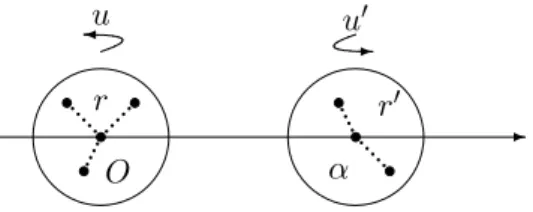
2.3 Compactness in the case of two interacting molecules

Now that we have identified the critical points at infinity for the mountain pass method, the next step is to show that min-maxing paths cannot approach these critical points. We study here the case of two interacting molecules with fixed nuclei. The parameters are then

• the distance between the two molecules (denoted by α in the sequel), • the orientation of each molecule (represented by two rotations u and u0_),

• the electronic wavefunction.

... ... -O ... ¾u u_-0 r _r0 α ... .. .. .. . ... .

Figure 2: Two molecules with fixed nuclei. So we consider r = (r₁, ..., r_m) ∈ B(0, R₀)m_{and r}0 _{= (r}0

1, ..., rm0 0) ∈ B(0, R₀)m 0

such that r1 = r01 = 0, ri 6= rj and r0i 6= r0j for i 6= j, and some z = (z1, ..., zm),

z0 _{= (z}0

1, ..., zm0 0). We denote by Z = (z, z0), and introduce

where ~v is a fixed vector of norm 1, α ∈ R, and u, u0 _{are rotations in R}3_{. We}

have used the notation u · r = (u · r₁, ..., u · r_m). We suppose now that N = |Z| and define

EN(α, u, u0, Ψ) := EN(R(α, u, u0), Ψ). In [25], it is proved that EN _{admits a minimum on R × (SO}

3(R))2× SHa1(R3N).

As in the previous sections, we shall assume that EN possesses two local minima M and M0_{. Up to a rotation of each molecule, we may suppose that α(M ) > 0}

and α(M0_{) > 0. We then consider}

c = inf

γ∈Γt∈[0;1]max E

N_(γ(t))

where Γ is the set of all the continuous functions γ : [0; 1] → X := (0; +∞) × (SO₃(R))2_{× SH}1

a(R3N) such that γ(0) = M and γ(1) = M0.

2.3.1 The mountain pass method

We begin this section by stating a result which is the analogue of Theorem 4 in this special setting.

Theorem 5. We have

• either there exists a critical point (α, u, u0, Ψ) of EN on X, such that HN(R(α, u, u0), Z) · Ψ = c · Ψ, c = λN₁ (R(α, u, u0), Z), • or c = min©EN1_{(r, z) + E}N2_(r0_{, z}0_{), N} 1+ N2= N ª .

Roughly speaking, the non compactness of min-maxing sequences is related to the existence of two gradient lines going from a local minimum to some critical point at infinity of index 0. The idea is that an ”optimal path” has to follow these lines, and then to connect the two critical points at infinity. Since the molecule is split here into two independent parts, the problem is now to find two mountain pass paths connecting each configuration of the two molecules – two similar problems of lower dimension. When the position of the nuclei in each molecule is fixed, these paths can be obtained by only applying some rotations. In other words, the minima always belong to the same connected component and this is why the situation will be simpler in this setting. When the position is not fixed, even if we may assume the existence of such paths (by induction), the situation is much more complicated and we hope to come back to this more general issue in the future.

The proof of Theorem 5 is very similar to the one of Theorem 4, and will be ommitted.

In order to prove that the second case in Theorem 5 does not happen, we need some information on the directions on which the energy decreases near the critical points at infinity. We shall thus need an expansion of the interaction energy between the two molecules when α grows. The terms involving in these expansion are classical. Let us first recall the definitions of the first multipoles.

Definition 2. Let be R = (R1, ..., RM) ∈ Ω, Z = (Z1, ..., ZM), and ρ ∈

L1_(R3_{) ∩ S(R}3_{\ {R}

j}) a non negative function such that

R

R3ρ = N > 0. Then 1. the total density of charge is the measure ˜ρ := ρ −PM_j=1Z_jδ_Rj. The total

charge is q :=R_R3ρ = N − |Z|,˜

2. the dipole moment is the vector P := R_R3x˜ρ(x) dx =

R

R3xρ(x) dx −

P_M

j=1ZjRj,

3. the quadrupole moment is the matrix Q :=R_R3

¡ xxT ₋ 1 3|x|2I ¢ ˜ ρ(x) dx. When ρ is the electronic density associated to some eigenstate Ψ, we shall use the notations ρΨ, ˜ρΨ, PΨ and QΨ.

This multipoles will be used in the expansion of the interaction energy. To illustrate this point, we give here the following

Lemma 2. We assume that N1 and N2are such that N1+N2 = N , EN1(r, z) <

ΣN1_{(r, z) and E}N2_(r0_{, z}0_{) < Σ}N2_(r0_{, z}0_{). Let ψ}

1 and ψ2 be two ground states of

respectively HN1_{(r, z) and H}N2_(r0_{, z}0_{). Denoting}

Ψ(α, u, u0) = (u · ψ1) ∧ (τα~v· u0· ψ2), we have EN¡R(α, u, u0), Ψ(α, u, u0)¢= EN1_{(r, z) + E}N2_(r0_{, z}0₎ +q1q2 α + q2 uP₁· ~v α2 − q1 u0_P 2· ~v α2 + (uP₁) · (u0_P 2) − 3(uP1· ~v)(u0P2· ~v) α3 +3(q2uQ1u T _{+ q} 1u0Q2u0T)v · v 2α3 + O µ 1 α4 ¶ for all u, u0 _{∈ SO}

3(R) and when α goes to +∞.

In this result, qk, Pkand Qkare respectively the total charge, the dipole and

the quadrupole moment associated to the electronic densities ρ_k of the states ψk.

The terms of this expansion can be interpreted respectively as the ener-gies of the molecules, and the interaction energy between them, which decom-poses into the charge/charge (1/α), dipole/charge (1/α2_{), dipole/dipole and}

charge/quadrupole (1/α3_{) terms.}

We are now able to state our main compactness results. As mentioned above, we had to add some hypothesis about the molecules ”at infinity”, concerning their multipoles in their ground state.

2.3.2 The case of charged molecules at infinity

Our first result will concern the case of monopoles at infinity, that is to say when the molecules are charged.

Theorem 6 (Charged molecules at infinity). Let us assume that EN1_{(r, z) + E}N2_(r0_{, z}0_{) = min}©_En1_{(r, z) + E}n2_(r0_{, z}0_{), n}

1+ n2 = N

ª (9) for some N1 and N2 with (N1− |z|)(N2− |z0|) 6= 0.

Then the case 2) in Theorem 5 does not happen. Therefore c is a critical value of EN _{on X.}

Remark – By (9), we have for instance

µ := EN1_{(r, z) − E}|z|_{(r, z) < E}|z0|_(r0_{, z}0_{) − E}N2_(r0_{, z}0_{) := µ}0

for some N1, N2 such that N1+ N2 = N and N1 < |z|. This can be viewed as

a comparison between oxydo-reduction potentials. So (9) will be probably true if one molecule is a oxydant and the other is a reductor.

2.3.3 The case of neutral molecules with dipole moments at infinity If the two molecules at infinity are neutral, the first term involving in the expansion of the interaction energy is the dipole/dipole term. This is why we shall now consider the case of molecules that possess some dipole moment in their ground state (experiment suggests that this is the case for every non symmetric molecule).

Let us introduce the following definition

Definition 3. Let be R = (R1, ..., RM) ∈ Ω, Z = (Z1, ..., ZM) and N > 0 such

that λN₁ (R, Z) < ΣN(R, Z). We shall say that the molecule (R, Z, N ) possesses a dipole moment at its ground state if PΨ6= 0 for all ground state Ψ.

Since V := ker¡HN_{(R, Z) − E}N_{(R, Z)}¢ _{is finite dimensional, let us notice}

that this implies min{|P_Ψ|, Ψ ∈ V, ||Ψ||_L2 = 1} > 0.

We then have the following result:

Theorem 7 (Neutral molecules with dipole moments at infinity). Let us assume that

(H1) E|z|_{(r, z) + E}|z0_|

(r0_{, z}0_{) < E}N1_{(r, z) + E}N2_(r0_{, z}0_{) for all N}

1, N2 such that

N₁+ N₂= N and (N₁− |z|)(N₂− |z0_{|) 6= 0,}

(H2) the two molecules (r, z, |z|) and (r0, z0, |z0|) possess a dipole moment at their ground state,

(H3) E|z|_{(r, z) or E}|z0_|

(r0_{, z}0_{) is non-degenerated.}

Then the case 2) in Theorem 5 does not happen. Therefore c is a critical value of EN _{on X.}

Remark – (H3) is a purely mathematical restriction that simplifies the proof.

Let us explain the general idea of the proof. Recall that the dipole/dipole interaction energy can be written F (P, P0_)/α3 _{(see Lemma 2). It is shown in}

Appendix 2 that the critical points of F which have a non-negative energy have a Morse index which is at least one. If a path approaches a critical point at infinity then, to pull down the energy along the path, one may use either the rotations of the molecules if the dipole/dipole interaction energy is positive (thanks to this Morse index information on F ), or the distance between them if it is negative (because α 7→ F (P, P0_)/α3 _{is then increasing). This is why}

min-maxing paths do not approach the critical points at infinity, and give thus a compact Palais-Smale sequence. Obviously, this general idea does not suffice to lead the proof and there are some other difficulties (essentially due to the complexity of the model) that are explicited in the next section.

Remark – This general information on the Morse index is probably true for the others multipoles interaction energies, a fact that could be used to treat the general case.

3

Proofs

3.1 Proof of Theorems 2 and 3

3.1.1 Preliminaries

We shall use the following lemma, which is an adaptation of results in [15, 16, 11, 12, 13], and which is proved in Appendix 1.

Lemma 3. Let ΨR be an eigenfunction associated to the eigenvalue λNd(R, Z)

and ρR be the electronic density. We introduce ²R = ΣN(R, Z) − λN_d(R, Z).

Then

1. ρR satisfies the inequation

−1 2∆ρR+ VRρR+ ²RρR≤ 0. (10) 2. With R1(²) := max ³ R0+ 1, R0+2N p_² ´ and C(²) := ∪p_j=1{x, |x − Xj| =

R1(²)}, and if r > 2R1(²R), then we have

ρR(x) ≤ ||ρR||L∞_(C(²R)) p X j=1 e− √ ²R/p(|Xj−x|−R1(²R)) ≤ p||ρR||L∞_(C(²R))e− √ ²R/p(δ(x)−R1(²R)) ₍₁₁₎ ≤ M e− √ ²R/p(δ(x)−R1(²R))_,

on U(R1(²R)), where δ(x) = min{|x − Xj|, j = 1, ..., d}, and M =

M (p, N, R1(²R)).

The explicit bound (11) has been written in order to show the dependence of all the constants with regard to ²_R. It is clearly not optimal. It shows a non-isotropic exponential decay of the electronic density, which will be uniform if ²R 9 0. This type of bounds is studied in the work of Agmon [1] and we

do not know if one can use his formalism to obtain the same result. Isotropic exponential bounds for N -body eigenfunctions are frequently seen in the litera-ture, but surprising is the fact that such non-isotropic bounds has not yet been noticed.

The next two lemmas will be useful to prove the exponential decay of The-orem 2.

Lemma 4. For all α > 0, there exists a constant M = M (α, N, R0) such that

tR(x) ≤ M

Z

B(x,α)

ρR(y) dy

on U(R0+ 1/2 + α).

Proof of Lemma 4 – see [16].

Lemma 5. For all j = 1, ..., p, d ≥ 1 and n ≤ |z_j|, we have inf

rj∈ωj

(Σn(r_j, z_j) − λn_d(r_j, z_j)) > 0. Proof – We have

Σn(rj, zj) − λnd(rj, zj) = ˜Σn(rj, zj) − ˜λnd(rj, zj)

where ˜λn_d(rj, zj) and ˜Σn(rj, zj) are the dth eigenvalue and the bottom of the

essential spectrum of the Hamiltonian with the nuclei interaction removed ˜ Hn(r_j, z_j) = n X i=1 µ −1 2∆xi+ Vrj(xi) ¶ + X 1≤i<j≤n 1 |xi− xj| . By Zhislin’s Theorem, it is known that

˜

Σn(r_j, z_j) − ˜λn_d(r_j, z_j) > 0

for all rj ∈ ωj and, since this function is continuous with regard to rj,

inf

rj∈ωj

(Σn(rj, zj) − λnd(rj, zj)) > 0.

In the next result, we use both HVZ and Zhislin’s Theorems. This lemma will be useful in the proof of Theorem 2 to construct test functions.

Lemma 6. If the minimum min    p X j=1 λNj δj (rj, zj), N1+ ... + Np = N, p Y j=1 δj = d   . is attained for N1, ..., Nj and δ1, ..., δp, then necessarily

λNj

δj (rj, zj) < Σ

Nj

δj (rj, zj)

Proof of Lemma 6 – Remark that by definition λ0

δj(rj, zj) < Σ

0_(r

j, zj) =

+∞ for all δ_j. We argue by contradiction and suppose that there exists a k such that Nk > 0 and λN_δkk(rk, zk) = ΣNk(rk, zk) = ENk−1(rk, zk). Theorem 1

implies Nk ≥ |zk| + 1. Since

P_p

j=1(Nk− |zk|) = N − |Z| ≤ 0, there exists a

l 6= k such that Nl < |zl|. We then let δj0 = δj, Nj0 = Nj for j /∈ {k, l}, δ_k0 = 1,

N0 k= Nk− 1, δ0l= δkδl, and Nl0 = Nl+ 1. We obtain p X j=1 λNj δj (rj, zj) − p X j=1 λNj0 δ0 j (rj, zj) = λ Nl δl (rl, zl) − λ Nl+1 δ0 l (rl, zl) ≥ ENl_(r l, zl) − λN_δ0l+1 l (rl, zl) = ΣNl+1_(r l, zl) − λN_δ0l+1 l (rl, zl) > 0

since Nl+ 1 ≤ |zl| (Zhislin Theorem), which is a contradiction.

3.1.2 Proof of Theorem 2

We are now able to prove Theorem 2.

We first prove 2). Suppose that the right hand side is attained for some N1, ..., Nj and δ1, ..., δp such that N1+ ... + Np = N and

Q_p

j=1δj = p. For the

sake of simplicity, we may assume that N_j > 0 for all j = 1, ..., p. By Lemma 6 and Theorem 1, there exist eigenfunctions Ψk_j ∈ L2_a(R3Nj_{) satisfying}

HNj_(r

j, zj)Ψkj = λkNj(rj, zj)Ψkj,

Z

R3Nj

Ψk_jΨl_j = δ_kl for all j = 1, ..., p and k = 1, ..., δj. If

Vj = span(Ψkj, k = 1, ..., δj) ⊂ L2a(R3Nj) then we have max Ψ∈Vj, ||Ψ||2_L=1 hHNj_(r j, zj)Ψ, Ψi = λN_δjj(rj, zj).

We now consider a sequence tn→ +∞ such that limn→+∞λNd(R(tn), Z) =

lim sup_t→+∞λN

d(R(t), Z). If Ψ ∈ L2(R3N), we introduce

Ψk,n_j = τ_Xj(tn)· Ψk_j ˜

V_jn= span(Ψk,n_j , k = 1, ..., δj) ⊂ L2a(R3Nj).

(we recall that τv is the translation by v).

Now, let be

Wn= ˜V1n∧ · · · ∧ ˜Vpn= span(Ψk11,n∧ · · · ∧ Ψ

kp,n

p , 1 ≤ kj ≤ δj)

which is a space of dimensionQd_j=1δj = d. If

Ψ = X

1≤kj≤δj

ck1,...,kpΨ

k1,n

and P|ck1,...,kp|2= 1, we have hHN(R, Z)Ψ, Ψi = p X j=1 X 1≤kj≤δj |c_k1,...,kp|2hHNj_(r j, zj)Ψkjj,n, Ψ kj,n j i + en

where en is the interaction energy between the p molecules. It is the sum of

three terms

en= e1n+ e2n+ e3n.

e1_nis the interaction between electrons in different molecules, and contains terms like Z Z _(Ψk_j1 j1 Ψ k0 j1 j1 )(x, ...)Ψ k_j2 j2 Ψ k0 j2 j2 )(y, ...) |x − y + Xj2(tn) − Xj1(tn)| dx dy.

with j1 6= j2. e2n is the interaction between electrons and nuclei of different

molecules, and contains terms like

Z Z _z j2,i(Ψ k_j1 j1 Ψ k0 j1 j1 )(x, ...) |x − rj2,i+ Xj2(tn) − Xj1(tn)| dx dy

with j16= j2. Finally, e3nis the interaction between nuclei of different molecules

e3_n= X j1<j2 X 1≤kj≤mj z_j1,kj1z_j2,kj1 |rj1,k_j1 − rj2,k_j2 + Xj2(tn) − Xj1(tn)| . It is now easy to see that each of this term tends to 0 as n → +∞.

By definition, we have λN_d(R, Z) ≤ _P max |c_k1,...,kp|2₌₁hH N_{(R, Z)Ψ, Ψi} ≤ p X j=1 max P |c_k1,...,kp|2₌₁ X 1≤kj≤δj |ck1,...,kp|2λ Nj kj(rj, zj) + max en ≤ p X j=1 λNj δj (rj, zj) + max en.

We may now pass to the limit as n → +∞ in this inequality and obtain the bound lim sup t→+∞ λ N d(R(t), Z) ≤ min    p X j=1 λNj δj (rj, zj), N1+ ... + Np = N, p Y j=1 δj = d   .

We then prove simultaneously 1) 3) 4) by induction on N = 1, ..., |Z|. For N = 1, it is known that

Σ1(R, Z) = E0(R, Z) = X

1≤i<j≤M

ZiZj

|Ri− Rj|

and so lim t→+∞Σ 1_{(R(t), Z) =} p X j=1 X 1≤k<l≤mj zj,kzj,l |r_j,k− r_j,l| = p X j=1 E0(rj, zj). As a consequence lim inf t→+∞ ¡ Σ1(R(t), Z) − λ1_d(R(t), Z)¢ ≥ p X j=1 E0(r_j, z_j) −  λ1 d(r1, z1) + p X j=2 E0(r_j, z_j)   = E0(r1, z1) − λ1d(r1, z1) = Σ1(r1, z1) − λ1d(r1, z1) and inf ri∈ωi lim inf t→+∞ ¡ Σ1(R(t), Z) − λ1_d(R(t), Z)¢≥ inf r1∈ω1 ¡ Σ1(r1, z1) − λ1d(r1, z1) ¢ > 0 by lemma 5. The uniform exponential decay is then a consequence of lemmas 3 and 4.

Let tn→ +∞ be such that limn→+∞E1(R(tn), Z) = lim inft→+∞E1(R(t), Z),

and φn_{∈ L}2_(R3_{) be such that}

H1(R(tn), Z)φn= E1(R(tn), Z)φn.

By the uniform exponential decay, we may write φn ₌ Pp

j=1φnj + αn where supp(φn j) ⊂ B(Xj, rn/3), and ||αn||H1 → 0. Then hH1(R(t_n), Z)φn, φni = p X j=1 h ˜H1(r_j, z_j)φn_j, φn_ji + p X j=1 X 1≤k<l≤mj zj,kzj,l |rj,k− rj,l| + e_n

where ˜H is the Hamiltonian with the nuclei interaction removed, and en → 0.

We have p X j=1 h ˜H1(r_j, z_j)φn_j, φn_ji ≥ X j=1,...,p ˜ E1(r_j, z_j)||φn_j||2_L2 ≥ min j=1,...,p ˜ E1(rj, zj)   X j=1,...,p ||φn_j||2_L2   so hH1(R(tn), Z)φn, φni ≥ min j=1,...,p ˜ E1(rj, zj) + p X j=1 X 1≤k<l≤mj zj,kzj,l |r_j,k− r_j,l| = min    p X j=1 ENj_(r j, zj), N1+ ... + Np = 1   

and finally lim t→+∞E 1_{(R(t), Z) = min}    p X j=1 ENj_(r j, zj), N1+ ... + Np= 1   .

Let us now assume that 1) 3) 4) have been proved for N − 1 < |Z|. We have ΣN(R, Z) = λN −1₁ (R, Z) so lim t→+∞Σ N_{(R(t), Z) = min}    p X j=1 ENj_(r j, zj), N1+ ... + Np = N − 1    = p X j=1 ENj_(r j, zj)

for some N₁, ..., N_p. ButPp_j=1(|z_j| − N_j) = |Z| − (N − 1) > 0 so there exists a k such that Nk< |zk|. We then have, for all d ≥ 1,

lim inf t→+∞ ¡ ΣN(R(t), Z) − λN_d (R(t), Z)¢ ≥ p X j=1 ENj_(r j, zj) −  λNk+1 d (rk, zk) + p X j=1, j6=k ENj_(r j, zj)   = ENk_(r k, zk) − λN_dk+1(rk, zk) = ΣNk+1(rk, zk) − λN_dk+1(rk, zk) and inf ri∈ωi lim inf t→+∞ ¡ ΣN(R(t), Z) − λN_d(R(t), Z)¢ ≥ inf j = 1, ..., p n ≤ |zj| inf rj∈ωj (Σn(rj, zj) − λnd(rj, zj)) > 0

by lemma 5. The uniform exponential decay 4) is then a consequence of lemmas 3 and 4.

We now prove the inequality lim inf t→+∞E N_{(R(t), Z) ≥ min}    p X j=1 ENj_(r j, zj), N1+ ... + Np = N    by using a variant of classical N -body geometric methods for Schr¨odinger op-erators [30, 29, 19], which is used in [10].

Let t_n → +∞ be such that lim_nEN_(R(t

n), Z) = lim inftEN(R(t), Z), and

Ψn an associated sequence of ground states, with densities ρΨn and tΨn. We

denote Rn _{= R(t}

n) and Xjn = Xj(tn). Due to the uniform exponential decay,

one has lim n→+∞ Z U(tn/3) ρ_Ψn = lim n→+∞ Z U(tn/3) t_Ψn = 0. (12)

Let ξn ∈ C∞(R3, [0; 1]) be a cutoff function such that ξn ≡ 0 on U(tn/3),

ξ_n≡ 1 on R3_{\ U(t}

n/3 − 1), and ||∇ξn||∞≤ 1, ||∆ξn||∞≤ 2. We then introduce

χn(x1, ..., xN) =

Q_N

i=1ξn(xi) and ˜Ψn= χnΨn. Using (12), it is then easy to see

that ||Ψn− ˜Ψn||H1 → 0, and HN(Rn, Z) · ˜Ψn− λN1 (Rn, Z) · ˜Ψn = − N X i=1 (2∇xiχn· ∇xiΨn+ Ψn∆xiχn) → 0 in L2(R3N), EN(Rn, ˜Ψ_n) − λN₁ (Rn, Ψ_n)|| ˜Ψ_n||_L2_(R3N₎= N X i=1 Z |Ψ_n|2|∇_xiχ_n|2 → 0. Now, we may write ξ_n=Pp_j=1ξnj where Supp(ξnj) ⊂ B(Xj, tn/3), and

˜ Ψ_n= X 1≤kj≤p ξk1 n (x1) · · · ξnkN(xN)Ψn:= X 1≤kj≤p Ψk1,...,kN n . Since the Ψk1,...,kN

n have disjoint supports,

| ˜Ψn|2= X 1≤kj≤p |Ψk1,...,kN n |2, EN(Rn, ˜Ψn) = X 1≤kj≤p EN(Rn, Ψkn1,...,kN), ¡ HN(Rn, Z) − λN₁ (Rn, Z)¢· Ψk1,...,kN n → 0 in L2_(R3N_{) for all k}

1, ...kN. To end the proof of Theorem 2, it suffices to bound

EN_(Rn_{, ˜Ψ}

n) from below by the appropriate constant.. We now fix k1, ..., kN and

introduce C_j = {i, k_i = j}, N_j = |C_j|. Remark that Ψk1,...,kN

n is antisymmetric

in (xi)i∈Cj for all j = 1, ..., p. Then

EN(Rn, Ψk1,...,kN n ) = p X j=1  X i∈Cj Z 1 2|∇xiΨkn1,...,kN|2− X i∈Cj Z V˜rj(xi)|Ψkn1,...,kN|2 + X k,l∈Cj Z |Ψk1,...,kN n |2 |xk− xl| + E 0_(r j, zj)   + en where en= X 1≤j6=j0_≤p  X i∈Cj Z Vr˜j0(xi)|Ψ k1,...,kN n |2+ X i∈Cj X i0_∈C j0 Z |Ψk1,...,kN n |2 |xi− xi0|   + e0 n, e0

n being the interaction energy between nuclei in different molecules, which

easily tends to 0 as n → +∞. Now |en| ≤ X 1≤j6=j0_≤p  X i∈Cj Z 3|zj| tn |Ψk1,...,kN n |2+ 3 X i∈Cj X i0_∈C j0 Z |Ψk1,...,kN n |2 tn  +e0 n→ 0

as n → +∞. Finally, since Ψk1,...,kN

n is antisymmetric in (xi)i∈Cj for all j =

1, ..., p and thanks to the translation invariance of the Hamiltonian, EN(Rn, Ψk1,...,kN n ) ≥   p X j=1 ENj_(r j, zj)   ||Ψk1,...,kN n ||2L2 + e_n.

Passing to the limit, we obtain lim n→+∞E N_(Rn_{, ˜Ψ} n) ≥ min    p X j=1 ENj_(r j, zj), N1+ · · · Np = N    which ends the proof of Theorem 2.

3.1.3 Proof of Theorem 3

The proof uses exactly the same N -body geometric method as the end of the proof of Theorem 2, but with λN

1 (Rn, Z) replaced by λNd(Rn, Z). If we suppose

that limn→+∞λN_d(Rn, Z) = c, then passing to the limit and using Theorem 2

c ≤ lim sup n→+∞ λ N d(Rn, Z) ≤ ΛNd(r, z). We have _¡ HN(Rn, Z) − c¢· Ψk1,...,kN n → 0 in L2_(R3N_{) for all k}

1, ...kN. Since all the interaction terms tend to 0 (see the

proof of Theorem 2), we obtain   p X j=1 HNj_(Xn j + rnj, zj)Cj − c   · Ψk1,...,kN n → 0

where the Hamiltonian HNj_(Xn

j + rnj, zj)Cj acts on the variables (xi)i∈Cj. Due

to the translation invariance, we obtain   p X j=1 HNj_(rn j, zj)Cj− c   · ˜Ψk1,...,kN n → 0 where ˜Ψk1,...,kN

n (x1, ..., xN) = Ψnk1,...,kN(X_kn_i + xi). But due to the exponential

decay of Ψn, ˜Ψkn1,...,kN is precompact in H1(R3N) and converges up to a

subse-quence to some ˜Ψk1,...,kN such that

  p X j=1 HNj_(r j, zj)Cj   ˜_Ψk1,...,kN _{= c · ˜Ψ}k1,...,kN_.

We thus have either c is an eigenvalue of ³Pp_j=1HNj_(r

j, zj)Cj

´

on the tensor product Np_j=1L2

Lemma 7. We have σ³Pp_j=1HNj(r j, zj)Cj ´ =Pp_j=1σ¡HNj(r j, zj)Cj ¢ so that σ_ess³Pp_j=1HNj(r j, zj)Cj ´ = [Σ; +∞) with Σ = min    X j6=j0 ENj_(r j, zj) + ΣNj0(rj0, zj0), 1 ≤ j0 ≤ p    > ΛN_d(r, z) for all d ≥ 1.

Proof of Lemma 7 – The fact that the spectrum of Pp_j=1HNj_(r

j, zj)Cj

is the sumPp_j=1σ¡HNj(r

j, zj)Cj

¢

is standard (see for instance [27], Theorem VIII-33). Suppose now that Σ = P_j6=j0ENj_(r

j, zj) + ΣNj0(rj0, zj0) for some 1 ≤ j0 ≤ p. If λN_dj0(rj0, zj0) < ΣNj0(rj0, zj0) then obviously Σ > ΛNd(r, z). If λNj0 d (rj0, zj0) = ΣNj0(rj0, zj0) then Σ > ΛNd(r, z) by lemma 6. As a consequence, if c is an eigenvalue of ³Pp_j=1HNj_(r j, zj)Cj ´ , it is nec-essary below its essential spectrum. It is then easy to see that this implies

˜ Ψk1,...,kN _∈ p O j=1 ker ³ HNj_(r j, zj) − λN_δjj(rj, zj) ´ Cj for some λNj δj (rj, zj) < Σ Nj_(r j, zj). Now, we have ||Ψn− τn· Ψ||H1 a(R3N)→ 0 where Ψ = P k1,...,kNΨ˜ k1,...,kN_. 3.2 Proof of Theorem 4

We may suppose c > max(EN_{(R, Ψ), E}N_(R0_{, Ψ}0_)).

Let us first prove the equality c = c0_{. Indeed, c}0 _{≤ c is obvious. Let be}

r_n ∈ R a sequence such that m_n := max_t∈[0;1]EN_(r

n(t), Z) → c0 as n → +∞.

For each n ∈ N, we define c_n= inf ψ∈ΓΨ max t∈[0;1]E N_(r n(t), ψ(t)) Γ_Ψ=©ψ ∈ C0([0; 1], SH_a1(R3N)), ψ(0) = Ψ, ψ(1) = Ψ0ª.

We may now apply the methods of [8] to obtain some sequences t_k∈ [0; 1] and (Ψ_k)_k≥1 such that

1. lim k→+∞E N_(rn_(t k), Ψk) = cn, 2. HN(rn(tk), Z) · Ψk− EN(rn(tk), Ψk) · Ψk→ 0 in L2(R3N), 3. EN(rn(tk), Ψk) ≤ λN1 (rn(tk), Z) + ²k, lim k→+∞²k= 0

1, 2) correspond to the classical fact that one can obtain min-maxing sequences that are almost critical. On the other hand, 3) is a consequence of the less-known fact that one can obtain Palais-Smale sequences with Morse-type in-formation related to the dimension of the homotopy-stable class used in the min-max method, which is 1 here (paths are deformations of [0; 1]). Since we are in C = R2_{, eigenvectors always have an even Morse index and this is why}

λN

1 appears in 3) and not λN2 .

The fact that such a sequence (Ψ_k) is precompact in H1

a(R3N) is now a

sim-ple consequence of Theorem 1 - 4). Indeed, the compactness below the essential spectrum is nothing else but the Palais-Smale condition of EN _{with Morse-type}

information introduced in [14]. We have the following general lemma, whose proof is postponed until the end of the proof of Theorem 4.

Lemma 8. We assume that Z = (Z1, ..., ZM) is such that N ≤ |Z|. Let

(Rn_{, Ψ}n_{) be a sequence in Ω × SH}1 a(R3N) such that 1. Rn_{→ R ∈ Ω} 2. lim n→+∞E N_(Rn_{, Ψ}n_{) = c,} 3. HN(Rn, Z) · Ψn− EN(Rn, Ψn) · Ψn→ 0 in L2(R3N),

4. there exist d0≥ 1 and ²n→ 0 such that EN(Rn, Ψn) ≤ λNd0(R

n_{, Z) + ²} n.

Then (Ψn_{) is precompact in H}1

a(R3N) and converges, up to a subsequence, to

an eigenfunction Ψ of HN(R, Z) associated to λN_d(R, Z) with d ≤ d0.

Applying this result, we obtain, by passing to the limit as k → +∞, c ≤ c_n= λN₁ (r_n(t_n), Z) ≤ m_n

for some t_n∈ [0; 1] and so c = c0_.

We now prove the alternative of the Theorem. We introduce

Fc(R0) =   (R, Ψ) ∈ Ω × SHa1(R3N), X i6=j |Ri− Rj| ≤ R0, EN(R, Ψ) ≥ c    Γ(α) = ½ γ ∈ Γ, max t∈[0;1]E N_{(γ(t)) ≤ c + α} ¾ . We have the following alternative:

either there exist R0 > 0 and α > 0 such that, Fc(R0) ∩ γ([0; 1]) 6= ∅ for all

γ ∈ Γ(α),

or for all R0 > 0 there exists a min-maxing sequence γn∈ Γ such that Fc(R0)∩

First Case : there exist R0> 0 and α > 0 such that, Fc(R0)∩γ([0; 1]) 6= ∅

for all γ ∈ Γ(α).

Since (R, Ψ) and (R0_{, Ψ}0_{) do not belong to F}

c(R0), we may apply the

methods of [14] (Fc(R0) is a set which is dual to the homotopy-stable class

Γ(α) with boundary B = {(R, Ψ), (R0_{, Ψ}0_{)}) to obtain a sequence (R}n_{, Ψ}n_{) ∈}

Ω × SH1 a(R3N) such that 1. lim n→+∞d((R n_{, Ψ}n_{), F} c(R0)) = 0, 2. lim n→+∞E N_(Rn_{, Ψ}n_{) = c,} 3. lim n→+∞∇RE N_(Rn_{, Ψ}n_{) = 0,} 4. HN(Rn, Z) · Ψn− EN(Rn, Ψn) · Ψn→ 0 in L2(R3N), 5. EN(Rn, Ψn) ≤ λN₁ (Rn, Z) + ²n, lim n→+∞²n= 0

Remark that 2, 3, 4, 5) correspond to the fact that one can obtain min-maxing sequences that are almost critical, and with Morse-type information. On the other hand, 1) is the consequence of the duality theory developed in [14] that enables to locate the critical points.

Due to 1), P_i6=j|Rn_i − Rn_j| is bounded. Up to a translation, we may sup-pose Rn _{→ R ∈ Ω (since λ}N

1 (Rn, Z) → +∞ when d(Rn, ∂Ω) → 0 due to the

nuclei/nuclei repulsion). Now Ψn _{converges up to a subsequence to a Ψ in}

H1_(R3N_{) by lemma 8.}

Second Case : for all R0 > 0 there exists a min-maxing sequence γn∈ Γ

such that Fc(R0) ∩ γn([0; 1]) = ∅.

Let (r_n) be a sequence in R such that r_n → +∞. For each r_n, there exists a γn such that, for instance,

c ≤ max t∈[0;1]E N_(γ n(t)) ≤ c + 1 n

and Fc(rn) ∩ γn([0; 1]) = ∅. We now write γn(t) = (Rn(t), ˜Ψn(t)) and fix n. The

set Kn= {t ∈ [0; 1],

P |Rn

i(t) − Rnj(t)| ≤ rn} is a compact subset of [0; 1] such

that max EN(γ(Kn)) < c. We now introduce

Γ_Ψ = n

ψ ∈ C0([0; 1], SH_a1(R3N)), ψ_|Kn ≡ ˜Ψn_|Kn o

which is an homotopy-stable class of dimension 1 with boundary ˜Ψn_(K

n), and cn= inf ψ∈ΓΨ max t∈[0;1] E N_(R n(t), ψ(t)) (13) so that c ≤ c_n≤ c + 1 n.

Applying the methods of [14], we may find a sequence tk ∈ [0; 1] \ Kn and

Ψk