Introduction 3
Overview . . . 4
Common definitions . . . 6
1 Discipline aggregation, manipulation and decisiveness 8 1.1 The combined format for sports climbing . . . 11
1.2 Formal description of the setting . . . 14
1.3 Manipulation in the discipline aggregation framework . . . 17
1.4 The likelihood of undesirable profiles . . . 21
1.5 Impossibilities that suggest a trade-off between decisiveness and manipulability 23 1.6 How easy is it to determine whether or not to manipulate . . . 32
1.7 Final remarks on discipline aggregation . . . 38
2 Relieving the tension between neutrality and resoluteness using parallel uni-verses 43 2.1 Binary trees . . . 47
2.1.1 Families of binary trees . . . 48
2.1.2 Using binary trees to define social choice functions . . . 50
2.2 Identities and properties of tree based rules . . . 51
2.2.1 Singleton trees . . . 52
2.2.2 Parallel universe trees . . . 53
2.2.3 Argmax applied to trees . . . 57
2.3 Success of tree-based argmax rules as refinements . . . 59
2.4 Assessment of the possible universes method . . . 60
3 Maximally decisive social choice 62 3.1 The informational content of families of functions . . . 64
3.1.1 Examples of informational bases . . . 65
3.1.2 Informational functions that express positional scoring rules . . . . 68
3.2 Maximally decisive rules with respect to bases . . . 74
3.2.1 Borda and maximal decisiveness . . . 75
3.2.2 Finding maximally decisive rules . . . 78
3.3 Final remarks on maximally decisive social choice . . . 80
4 Domain restrictions and independence of irrelevant alternatives 83 4.1 Definitions . . . 84
4.3 The Blau equivalence . . . 87
4.4 Violating the Blau equivalence . . . 90
4.5 Blau’s impossibility . . . 93
4.6 Final remarks on domain restrictions and independence . . . 97
5 Combining ordinal and evaluative information in social choice 99 5.1 The preference-approval model . . . 101
5.2 An impossibility in aggregating preference-approvals . . . 103
5.3 Possibilities from relaxing decomposability . . . 106
5.3.1 Relaxing the decomposability of the approval aggregation . . . 107
5.3.1.1 Well-behaved approval aggregators . . . 107
5.3.1.2 Maximally discriminating approval aggregators . . . 108
5.3.1.3 Relaxing decomposability with three or more alternatives 109 5.3.2 Relaxing decomposability between rankings and approvals . . . 110
5.3.2.1 Shortlist by elementary approval aggregators then rank . 111 5.3.2.2 Shortlist by non-decomposable approval aggregator . . . 111
5.3.2.3 Perform ranking aggregation then approve using ranking 112 5.3.2.4 Borda with a movable zero determined by the zero-line . 112 5.4 Extending the impossibility to more evaluation levels . . . 113
5.5 Final remarks . . . 115
Conclusion 119
This thesis is constructed from a series of articles concerning social choice theory. Some may be further specified as using the ideas of computational social choice theory. An anal-ysis of the words “social”, “choice”, “theory” and “computational” provides a general idea of the type of results contained within.
The word “theory” indicates that social choice theory is a formal field of study. In particular, this thesis is mostly concerned with mathematically formal issues—as opposed to empirical issues. However, although the work presented here is not dependent upon observations of the real world, it does involve modelling potentially real situations (this is explicitly the case for the simulations of Chapter 1).
The “social” part connects us to what is modelled, which is, in a rough sense, society. Of course, the concept of society is somewhat amorphous. In our models we attempt to capture one aspect of society that is relevant to collective choice: the preferences that each agent has. Such preferences can be expressed in many ways. The traditional approach of social choice theory, due to Arrow (1950), models society as a profile of ordinal preferences. This approach, and others that we consider, specifies precisely what are to be taken as the relevant possible states of society.
The “choice” part refers to some method for selecting or for ranking alternatives. For our purposes, such a method is a function whose domain is the possible states of society. The output of the function might be a chosen alternative. We call such functions social choice functions. Other functions may output a ranking over the alternatives. We call such functions social welfare functions. We are less concerned with descriptive accounts of how this is done in practice, and more with the normative properties of potential methods—we study what choices should be made by a social choice procedure.
We now come to “computational”. Problems of a social choice theoretic nature have been found to be applicable to problems traditionally associated with computer science. In the opposite direction, computational methods have been applied to the traditional problems of social choice theory. This cross-fertilisation has led to the birth of computational social choice. Interdisciplinary by nature, this field of study now treats many problems from dis-ciplines such as economics, computer science, articial intelligence, mathematics, political science and philosphy. Across these diverse settings, a number of specific techniques have been developed that have a particularly computational-social-choice-theoretic nature. Of par-ticular note is the application of the theory of computational complexity, which may (for example, negatively) show that a supposedly attractive social choice procedure is infeasible in practice (it may also be used positively to mitigate a negative result). Results using this
and other such concepts contribute to an understanding of the issues of social choice theory, not merely through performing simulations or calculations using computers, but thanks to the formal concepts and ideas of theoretical computer science.
Within the general framework of computational social choice theory, this thesis focuses on two main issues: how expressive the preferences of the agents are, and how decisive the choice procedure is. The first theme may be thought of as concerning how much information we have to deal with. The second theme considers what is done with this information. Now, the whole point of a choice procedure is to make a choice: if it often fails to do so, it will not be much use in practice. Along these lines, the second theme concerns how small can we make the choice set, or how refined the output ranking.
All of the chapters touch upon, to a lesser or greater degree, one or both of the themes of expressive-ness and decisive-ness. An overview of the specific content of each of the chapters follows.
Chapter summaries
Chapter 1 is intended to be an introduction to computational social choice theory that at the same time provides novel results. In it we apply the ideas of computational social choice theory to the problem of determining the winners for sports climbing at the 2020 Olympics. The method that will be used has been designed by the International Federation of Sports Climbing; we call this method inverse-Borda-Nash. Our nomenclature is intended to be descriptive—the method may be thought of as an inverse version of Borda scoring where the winning alternatives are those with minimal product scores.
Inverse-Borda-Nash has some undesirable behaviour: in particular, an athlete can increase a teammate’s ranking by performing worse; we say that it is manipulable. Simulations suggest that cases where manipulation can occur are not unlikely. Given that the proposed method is manipulable, one may wonder whether there is a different, better method for ranking the athletes. We formalise this problem by giving a mathematical description of the properties we want the method to satisfy. Unfortunately, we cannot satisfy all the desired properties at the same time: we have an impossibility. Impossibility results of this type abound in social choice theory to such an extent that there are recognisable families of methods that have been applied in attempt to lessen their negative implications. One such family is to use the theory of computational complexity from theoretical computer science to show that, although undesirable behaviour may be theoretically possible, it is not computationally feasible. In this vein, we prove that it is computationally hard to detect a manipulation for inverse-Borda-Nash.
The reason that our problem in Chapter 1 can be considered in terms of social choice theory is due to the information that is available to rank the athletes. The International Federation of Sports Climbing expressly wants the final ranking to be produced from an aggregation of three ordinal rankings. (Their reasons for this echo traditional concerns about the difficulty of making interpersonal comparisons of utility.) This allows us to make a recap of the traditional issues of computational social choice theory that is nonetheless novel. Further, we will also introduce what we believe to be a novel problem, at least in the way that it is formulated here: the issue of decisiveness. Intuitively, a single gold medallist is preferable to a tied situation with multiple gold medallists. This chapter presents the open problem of whether or not there is a tension between the decisiveness of the choice method and the other desirable properties. This problem seems to require a more formal definition of what it means for a choice method to be decisive or not.
Chapter 2 expressly attempts to make choice methods more decisive. The technique used is to count permutations—a technique inspired by the “parallel universe” tie-breaking version of instant runoff voting. In Chapter 2 we apply this technique to the class of tournament solutions. Tournament solutions take as input a complete directed graph over alternatives: this may be considered an informational restriction, as the majority preferences of society over the alternatives is less expressive than a full profile of preferences. Tournament so-lutions are apt to be made more decisive as they tend to output large sets. By counting permutations we certainly succeed in making them more decisive; however, depending on the precise manner in which this is done, we sometimes get non-intersecting choice sets, and it is not clear why we should prefer one choice method to another. Another drawback is the computationally demanding nature of our technique. Intuitively, tournament solutions provide large outcome sets in part because they do not use a lot of information. Using the techniques of this chapter we can create solution concepts that are much more decisive than those that are normally studied.
In Chapter 3 we look more generally at how decisive choice methods can be made given different informational assumptions. This combines the two major themes of expressiveness and decisiveness. The framework of this chapter is ordinal: we start with a full ordinal profile, and consider the effect of using less information than this. We develop a definition of maximal decisivenesswith respect to the available information. This is intended to identify whether or not a choice method is as selective as possible, given some natural restrictions. (An example restriction would be to require that the choice to be based on tournaments, as was the case in Chapter 2.) In particular, our definition of maximal decisiveness is designed around neutrality, the idea that all alternatives should be treated equally.
Chapter 4 considers information in two ways that are classic to social choice theory: inde-pendence of irrelevant alternativesand domain restrictions. Independence of irrelevant alternatives is a local informational restriction: instead of a global look at what information
is used by a rule or a family of rules, it concerns how much information from an individual profile is required to calculate part of the output of a social welfare function. With respect to social welfare functions, the strictest restriction of this type is binary independence, which requires that we can determine which of two alternatives is preferred in the output only by considering the pairwise comparisons of these two alternatives in the profile. This can then be weakened to ternary independence, quaternary independence, etc. It is known that under the full domain these are not real weakenings as they all collapse into binary independence (except for independence over the whole set of alternatives which is trivially satisfied). In Chapter 4 we investigate whether this still happens under restricted domains. A restricted domain is an express limit on the expressiveness: some profiles are supposed to not exist. We show that for different restricted domains the different levels of independence described above may or may not be equivalent, and specify when and to what extent different versions of independence collapse into the same condition.
Chapter 5 returns more speculatively to the question of what information should be col-lected from society. We contrast the traditional ordinal approach—that we have been using throughout the preceding chapters—with what we call the evaluative approach. The evalu-ative approach involves aggregating evaluations of the alternevalu-atives made by the agents. For example, approval voting, where society is supposed only to approve or disapprove each alternative, is evaluative. We prove an impossibility in combining the ranking and evalua-tive approaches. Our results suggest that there is a deep incompatibility between the two approaches.
Common definitions
The following definitions are applied consistently throughout the thesis, except for some slight variations in the first chapter.
Throughout we consider a finite set of objects A. With the exception of Chapter 1, this is called the set of alternatives. If is from this set that “society” makes a choice or creates a ranking. Typically |A| = m for some positive integer m. We refer to individual alternatives using a1, a2, . . . , am, a, b, c,. . . , x, y, z,. . .
The elements of A are variously ranked, approved, evaluated or chosen. We write W(A) for the set of complete and transitive binary relations, or complete preorders, over A. We use R to refer to elements of W(A). We typically use infix notation for binary relations, for example writing xRy instead of (x, y) ∈ R. A complete preorder R is a linear order if and only if R is also antisymmetric. We use L(A) for the set of linear orders over A. We use R∗ for the asymmetric part of R, i.e. for all x, y ∈ A, xR∗yif and only if xRy and not yRx. The
asymmetric part of a complete preorder is also a strict weak order, and the asymmetric part of a linear order is a strict linear order; we use P to denote such irreflexive relations when they do not correspond to some already defined R. We write W∗(A) and L∗(A) for the set of strict weak orders and the set of strict linear orders respectively. We sometimes display a (strict) linear order by simply writing a list starting with most preferred elements and ending with least preferred. For example, adbc corresponds to the linear order R such that aRd, dRb and bRc (or to the corresponding strict linear order P depending on context).
We also consider an index set N which, with the exception of Chapter 1, we refer to as the set of agents. Typically |N| = n. The set N may be thought of as the “members” of “society”. Different members of society may have different opinions concerning the different alternatives, which we typically model by assigning each agent a weak order preference over the alternatives. We call a full vector of preferences, denoted RRR∈ W(A)N, a profile. In general, we use bold typeface for vectors. For i ∈ N and RRR∈ W(A)N, we use R
i to refer to the ith coordinate of RRR. By (RRR−i, R′) we mean the profile RRRwith the coordinate Rireplaced by R′.
A social choice function takes preferences over alternatives and produces a non-empty set of choices; f : W(A)N → 2A\ /0. Sometimes the domain will be restricted or even modified en-tirely. A social welfare function takes preferences over alternatives and produces a ranking of alternatives; F : W(A)N→ W(A).
A permutation on some set X is an onto function g : X → X. We use typically consider per-mutations of alternatives or agents with the notation σ : A → A and ρ : N → N. We abuse no-tation and apply permuno-tations to preferences and profiles as follows. For R ∈ W(A) we write σ(R) = {(σ (x), σ (y)) : (x, y) ∈ R}. For (R1, . . . , Rn) ∈ W(A)N we write σ ((R1, . . . , Rn)) = (σ (R1), . . . , σ (Rn)) and ρ((R1, . . . , Rn)) = (Rρ(1), . . . , Rρ(n)).
Discipline aggregation, manipulation and
decisiveness
This chapter serves both as an introduction to the themes of this thesis, and as a recap of the basic ideas of social choice theory under a fresh interpretation. It is based upon joint work with Sebastian Schneckenburger that was presented at COMSOC 2018 and AAMAS 2019. In it we apply the traditional social choice framework to the problem of aggregating the competition results of multiple disciplines in a sports competition. This provides a recap of many of the theoretical results of social choice theory; in fact we will retread many of the historical advancements made within the field. Ultimately, our work raises the issue of decisiveness, one of the main themes of this thesis.
The 2020 Olympic Games in Tokyo will inaugurate ten new gold medals; one male and one female in each of five new events: karate, skateboarding, surfing, baseball and sports climbing. As it is the first time that these events will appear in the Olympics, for each event it is necessary to specify for the first time how the medal winners will be decided. This presents a particular problem for sports climbing, because sports climbing has not existed in a unique competition format before its introduction as an Olympic event. Instead, there are three prevalent types of competitive climbing: bouldering, lead-climbing and speed-climbing. It is these distinct types of sports climbing that we refer to as disciplines. Each discipline requires different skills and measures the performance of athletes using different methods. Thus sports climbing is to be a composite event, similar to the pentathlon—but the manner in which medal winners are determined for the pentathlon is by no means suitable here.
For sports climbing, it is desired that only the rankings of the athletes in each of the disci-plines are used to determine the medal winners. In contrast, for the pentathlon quantities such as time, height and distance, measured independently for each athlete, form the basis for the final ranking. Given the “only rankings” constraint, the problem of designing a pro-cedure for choosing the medal winners is similar to that of designing a propro-cedure of social choice theory. Of course, the terminology is different: what is traditionally the set of voters has become the set of disciplines; the set of candidates becomes the set of athletes. But the underlying problem is the same: how should we aggregate multiple rankings into a single, definitive ranking?
For the sports climbing event at the 2020 Olympics, the International Federation of Sports Climbing (2017) has decided to rank the athletes according to the product of their ranks in the disciplines. They have various reasons for this choice, which we will discuss later. Also, the method will be tested in some trial events before the Olympics in order to confirm is suitability. On the other hand, there are theoretical situations where the method gives undesirable results: it can produce ties among a large number of athletes, which cannot always be broken in an obvious manner; and it is potentially open to a type of manipulation. In social choice theory, undesirable possibilities are often called paradoxes. The most fa-mous example is Condorcet’s (1785) paradox, which shows that it is possible that a majority prefers a first alternative to a second, that a majority prefers the second to a third, and also that a majority prefers the third to the first.1 We will see another such majority cycle later in this chapter (Figure 1.1). Of course, just stating individual examples of undesirable be-haviour would be a somewhat haphazard method of analysis, a more general and principled method of analysis is preferable.
In order to assess all relevant possible procedures for determining the medal winners, one can try to encompass them in a single framework. In order to do so, we treat them as math-ematical functions from lists of rankings to a final output ranking. We call such functions discipline aggregators.2 The method of formalising social choice problems in this manner was pioneered by Arrow (1950); it allows us to assess the possible procedures for selecting medal winners based upon their formal properties.
There are a number of properties that a discipline aggregator may satisfy—following Arrow, in the academic literature on social choice theory such desirable properties are typically called axioms. We want our function to satisfy such desirable properties. For example, if a first athlete performs better than a second in all the disciplines, surely the first athlete should be ranked better than the second. On the other hand, there may be undesirable possibilities for certain functions, for example, a function may be manipulable in some way or another. The basic idea behind our definitions of manipulation is that, in certain situations, an athlete can aid a teammate by performing worse than they normally would have done.3 If such an situation is theoretically possible, an athlete may indeed perform such a manipulation in
1Other examples of so-called paradoxes include the Ostrogorski paradox (Rae and Daudt, 1976),
Anscombe’s paradox (Anscombe, 1976), and the multiple election paradox (Brams et al., 1998).
2Although “discipline aggregator” may be thought of as a synonym for “social welfare function”
mathemat-ically speaking, our nomenclature in this chapter serves as a reminder that there is a difference in interpretation here.
3This idea of manipulation is not an alias of some previously studied concept from social choice theory.
In particular, it is not simply Gibbard-Satterthwaite manipulation. Gibbard-Satterthwaite manipulation is “per-formed” by a discipline, and involves any possible change to the single ranking of this discipline. In contrast, the manipulations we consider in this chapter are “performed” by an athlete, and involve a restricted change to that athlete’s ranking throughout the whole profile.
reality, which we take to be an undesirable event. We want our function to preclude such possibilities.
A formal description of the problem also makes it easier to determine how often any given paradoxical situation will occur. This question has a potentially empirical character; however there is sometimes a lack of real life data: this can be the case for real-life preferences of agents, but is especially so for our particular discipline aggregation problem, as events using the combined format for sports climbing have only started to be run last year (2018). We can, however, perform simulations given some assumptions on how likely each possible state is (Garman and Kamien, 1968; Gehrlein and Fishburn, 1976).
We will give a few different definitions describing situations where a discipline aggregation function can be manipulated. Under our most permissive definitions of manipulation, only unreasonable functions can completely prevent such manipulation from occurring. That is, we prove an impossibility result: any function that prevents manipulation must violate some other desirable condition. Such a negative result, if accepted, seems to imply that some sort of trade-off must be made.
Impossibility results often arise in social choice theory,4 and there are many different tech-niques that have been developed in attempt to mitigate their negative conclusions. Perhaps the most direct attack against such a result is to argue that the identified conditions are not really necessary for a rule to be reasonable. For the most part, the properties we define are obviously desirable. The point of weakness is in our definitions of manipulation, which in-deed takes the place of the much discussed—and challenged—property of independence of irrelevant alternatives.5 Various weakened versions of this property have been proposed in the literature.
Indeed, with a slightly less permissive definition of when manipulation is possible, there are functions that satisfy our desirable properties. However, the function that exemplifies the possibility is, intuitively, not decisive enough. Although it satisfies our given properties, it is nonetheless an unreasonable rule. This can only occur because our given properties are quite weak—they are necessary for a rule to be reasonable, but not sufficient; precisely, they are missing a condition that ensures a minimal level of decisiveness.
This raises the issue of determining a condition that ensures a minimal level of decisiveness. Although the function exemplifying the possibility is intuitively indecisive, there is no formal specification of this property. It is not obvious how to define a reasonable condition of decisiveness that this function does not satisfy. In fact, there is an unreasonable, very strong decisiveness condition that we can impose: we can require that there are no ties at all in the
4Impossibility results are the subject of a Chapter 1 in the Handbook of Social Choice and Welfare
(Camp-bell and Kelly, 2002).
output; that a linear order is returned—this is known as resoluteness. With this property added, the impossibility reoccurs—the question is whether or not there is a sensible, weaker decisiveness condition will have the same effect. So, more generally, this chapter motivates further investigation of the concept of decisiveness; a project that will be continued in later chapters. Decisiveness is especially important for sports competitions, but remains important for social choice more generally: after all, the whole point of social choice theory is to make a choice!
The rest of this chapter proceeds as follows. In Section 1.1 we describe the proposed com-bined format for sports climbing, and give an example that shows that this method may be manipulated and may produce ties. We then provide a formal description of the ba-sic setting in Section 1.2, which contains most of the definitions necessary for our results. However, our description of the various types of manipulation we consider merits its own section: Section 1.3. Having completed our definitions, we then start our analysis in earnest. Our simulation results, in Section 1.4, show that the probability of ties under the proposed method is quite low, but that on the other hand there is a high potential for manipulation. Our theoretical results of Section 1.5 show that it is impossible to completely rule out manipu-lation, although we give a possibility for a plausible weakened version of our requirements concerning manipulation. This possibility, however, raises the issue of the decisiveness of discipline-aggregators. In Section 1.6 we prove that it is computationally hard to determine whether or not one can manipulate the proposed method if we allow the numbers of athletes and disciplines to increase. Section 1.7 concludes this chapter.
1.1
The combined format for sports climbing
For the 2020 Olympics the International Federation of Sports Climbing (2017) has devised the following combined format for sports climbing. Twenty athletes—of which each country can have up to two representatives—will be involved in the main event, which itself is split into two rounds. A qualification round first reduces the twenty athletes to six. These six finalists then compete in a separate final round to determine the medals. Although in the qualification round it is only necessary to select six athletes, in fact the procedure is identical to that of the final round and produces a full ordering over the contending athletes, the six best ranked are then selected.
So in each round a ranking over all the athletes is produced in the same manner: the con-tending athletes compete in all three disciplines, thereby producing three linear orders over the athletes. For each discipline any given specific athlete has a rank, which is the number of other athletes that defeat her plus one; a given athlete’s overall score is the product of the athlete’s ranks in each discipline. These product scores provide a final ordering over the
competitors, with lower scores being better. If two athletes receive the same score the tie can be broken in favour of the athlete that performs better than the other in more disciplines. That is, ties can be broken depending upon the so-called majority relation—we will see an example demonstrating how this works, but, in short: if more than two athletes receive the same score, ties are broken first by the transitive closure of the majority relation; where there are cycles, an external linear-order tiebreaker is used.
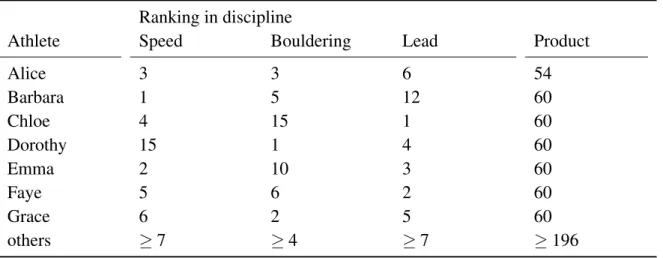
Unfortunately, the combined Olympic format may lead to tied situations if more than two athletes have the same product score and the pairwise comparisons form a cycle. Ties are problem for both rounds of the competition: in the final round, it is desirable to have a single gold winner; in the qualifying round, ties necessitate an extra method to determine which athletes progress. An example demonstrates the problem—Table 1.1 shows potential ranks of seven of the athletes and bounds on the ranks of the other thirteen athletes after the qualification round.
Table 1.1: Possible ranks of seven of the athletes after the first round of competition.
Ranking in discipline
Athlete Speed Bouldering Lead Product
Alice 3 3 6 54 Barbara 1 5 12 60 Chloe 4 15 1 60 Dorothy 15 1 4 60 Emma 2 10 3 60 Faye 5 6 2 60 Grace 6 2 5 60 others ≥ 7 ≥ 4 ≥ 7 ≥ 196
Only six of the athletes can proceed to the final round. This means that one of the six ath-letes with tied product scores—that is, one of the named athath-letes excepting Alice—must be eliminated from the competition (along with all the other unnamed athletes). However, it is not clear which of the six should be eliminated; when we compare each pair by which athlete defeats the other in more disciplines, we produce a cycle. This is displayed graphically in Figure 1.1: the athletes are represented by the first letter of their name, and an arrow points from one athlete to another if the first performs better than the second in more disciplines.
b c d e f g
Figure 1.1: The majority relation be-tween b, c, d, e, f and g—the athletes are labelled by the first letter of their name—given the results from Table 1.1.
The problem is that there is no Condorcet loser; that is, no athlete that is—in terms of majorities—defeated by all the other athletes. There is a parallel concept of a Condorcet winner: an athlete who defeats all other athletes according to the majority relation. The proposed method considers situations without Condorcet winners or losers as tied; thus the situation described in Table 1.1 requires the use of an external tiebreaker to decide which athlete is eliminated.6 Suppose that the external tiebreaker eliminates Barbara. If the re-maining athletes perform the same as in the first round, the ranks and products will be as displayed in Table 1.2.
Table 1.2: Predicted results if the named athletes except Barbara progress to the second round and perform the same as in the first round as given in Table 1.1.
Ranking in discipline
Athlete Speed Bouldering Lead Product
Alice 2 3 6 36 Chloe 3 6 1 18 Dorothy 6 1 4 24 Emma 1 5 3 15 Faye 4 4 2 32 Grace 5 2 5 50
6The IFSC will use a “seeding list” to break ties that are not resolvable by pairwise comparisons. Such a
seeding list is, in effect, an external linear order tiebreaker. For the final round the ranking of the qualification round will be used as a seeding list; for the qualification round a seeding list based on the prior qualification system will be used (Meyer, 2018).
There is a another potential problem here: manipulation. Suppose now that Alice and Chloe have the same nationality. The predicted results suggest that Alice will not win a medal, and certainly not the gold, while her teammate Chloe is predicted to win the silver. However, if Alice deliberately performs worse than Chloe in the speed competition and all other ranks remain the same, Chloe will become the unique gold medal winner with a product score of 12.7 Thus, national loyalty may lead Alice to manipulate. In doing so she spoils the result for Emma, whose efforts would normally have been enough for a gold medal.
The above example demonstrates two potential problems with the proposed method: ties and manipulation. We have not yet assessed how often these problems are likely to occur, that is, whether they are a likely problem in practice. Nor do we know whether or not these problems are in some sense necessary: it may not be possible to design other discipline aggregation functions which avoid them. To address these issues we require a more formal description of the setting.
1.2
Formal description of the setting
Denote by A = {a, b, c, . . . }, |A| = m the set of athletes and by N = {1, . . . , n} the set of disciplines. We suppose that m ≥ 3 and n ≥ 2; note that this covers the the specific cases of m= 6, m = 20 and n = 3. Denote the set of strict linear orders of A by L∗(A) and use P to denote a strict linear order over athletes. Denote and the set of complete preorders of A by W(A). and use R to denote a complete preorder over the athletes. We use R∗to denote the asymmetric part of R—note that P = R∗for some R.
All the athletes compete in each discipline i ∈ N, resulting in n strict linear orders Pi over A. A profile that summarises the results for each discipline is denoted by (P1, . . . , Pn) = PPP∈ L∗(A)N. A discipline aggregator F uses these results to produce a complete preorder over the competitors: F : L∗(A)N→ W(A).
Athletes have a rank for each discipline and for the output complete preorder. Formally, for an ordering R over competitors, the rank of a ∈ A is r(R)(a) = rR(a) = |{x ∈ A : xPa, x 6= a}| + 1. Note that r(R) = r(R∗). To simplify notation, for a discipline i ∈ N we write ri= r(Ri) = r(Pi) when the context makes it clear which profile was intended. Because lower ranks are better, Pi and the natural ordering on ranks are inverted: for all x, y ∈ A and i ∈ N, xPiy if and only if ri(x) < ri(y). Note that the output of a discipline aggregator
7The manipulation described here would be feasible in practice. The method used to produce the
speed-climbing ranking is a type of knockout tournament. Under the assumption that a defeats g and that c defeats f in the quarter finals, a will face c in the semifinals; if a deliberately loses then c will be guaranteed to be ranked at second or better at speed-climbing (International Federation of Sports Climbing, 2017).
can contain ties, though if two or more competitors are ranked first, no competitor is ranked second—a shared gold medal implies that no-one receives silver. We refer to athletes ranked first in the output as winners.
We can use a profile to make pairwise comparisons between athletes. For an arbitrary profile P
PPthe majority relation TPPP⊆ A × A is defined by, for all x, y ∈ A, x 6= y xTPPPy if and only if |{i ∈ N : xPiy}| ≥ |{i ∈ N : yPix}| .
The majority relation is connected regardless of the parity of |A|. It may not be transitive: for a binary relation Q we write Q+ for the transitive closure of Q, the smallest transitive relation that contains Q.
We now formally define the proposed discipline aggregator, insofar as it is determined by the profile of results. We call this function inverse-Borda-Nash,8 and denote it by ibn: L∗(A)N → W(A). Define the binary relation Q ⊆ A × A by
xQy iff
∏i∈Nri(x) > ∏i∈Nri(y) or
∏i∈Nri(x) = ∏i∈Nri(y) and xTPPPy.
Define ibn(PPP) = Q+∪ {(x, x) : x ∈ A}; because Q is connected this is a complete preorder.
Basic desirable properties
There are some basic desirable properties that a discipline aggregator F should satisfy. An athlete x ∈ A clearly beats y ∈ A in PPP if for all i ∈ N, xPiy. We say F satisfies the clear winner condition if whenever x clearly beats y in PPP, then for R = F(PPP) it is the case that
8This nomenclature is intended to be descriptive as it invokes Borda scores and the Nash product. The Nash
product is sometimes described as providing a middle ground between the utility maximisation of additive methods and the maxi-min of egalitarian methods. However, this is not the case for the proposed method because the Borda scores are inverted i.e. smaller numbers are better. If the scores were added, this inversion would have no effect, but this is not the case for multiplication. For example, according to inverse-Borda-Nash, an athlete with rankings (1,1,4) beats an athlete with (2,2,2); whereas for traditional Borda scores the opposite is true: (19,19,19) would be considered better than (20,20,17). It is seen as an advantage of the method that it favours specialists—it is preferred that the winner of the combined format is a potential winner of world-cups in some individual discipline, rather than a generalist (Meyer, 2018).
We are not aware of any specific precedent for inverse Borda-Nash. This may be because it would become an “anti-fairness” approach when applied to social choice or social welfare. However, it can be subsumed under well-known concepts; it is equivalent to a scoring rule with weights (log(m), log(m/2), . . . , log(m/m − 1), 0). The family of scoring rules are well studied within the literature, and the results of Proposition 1.1 below could be shown as corollaries to general results concerning this family.
xR∗y. The next two conditions impose symmetry restrictions, roughly speaking, they require that all athletes should be treated the same and that all disciplines should be treated the same. We say F satisfies athlete-neutrality if permuting the competitors in the profile similarly permutes the competitors in the output ranking: for any permutation σ : A → A, given PPPand PPP′such that for all a, b ∈ A, i ∈ N aPib⇔ σ (a)Pi′σ(b), then aF(PPP)b ⇔ σ (a)F(PPP′)σ (b). We say F satisfies discipline-neutrality if permuting the disciplines in the profile has no effect on the output ranking: for any permutation ρ : N → A, given PPPand PPP′such that for all i ∈ N, Pi= P′ρ(i), then F(PPP) = F(PPP′). Our last two properties limit how much a single discipline can determine the winner. For a discipline aggregator F, we say the gold is determined by i∈ N if, for any profile PPP, max(F(PPP)) = max(Pi). We say F is not determined if the gold is not determined by any i ∈ N. Similarly, for a discipline aggregator F, we say the gold is weakly determined by i ∈ N if, for any profile PPP and writing R = F(PPP), ri(x) = 1 implies rR(x) = 1. We say F is not weakly determined if the gold is not weakly determined by any i∈ N.
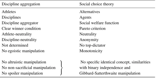
Each of these properties can be linked to axioms from social choice theory. The clear winner condition is called, for example, the “Pareto criterion” (Campbell and Kelly, 2002, p. 42).9 Athlete-neutrality becomes simply “neutrality”, whereas discipline-neutrality is known as “anonymity”. A discipline that determines the gold may be thought of as a “top-dictator”: an agent whose top ranked alternative must be the top ranked alternative in the output. Note that it is easier for a discipline aggregator to be not determined than not weakly determined; in particular, if a discipline aggregator satisfies discipline-neutrality then it is not determined, but may still be weakly determined.
As a final exposition of our definitions, we show that Inverse-Borda-Nash satisfies all these basic desirable properties.
Proposition 1.1. Inverse-Borda-Nash satisfies the clear winner condition, satisfies athlete-neutrality, satisfies discipline-athlete-neutrality, and is not weakly determined.
Proof. Clear winner: if an athlete is ranked better than another in all disciplines, it must have a smaller product of ranks, therefore will be ranked better in the output.
Athlete-neutrality: if we permute athletes, we also permute their product scores and the relation TPPP.
Discipline-neutrality: permuting disciplines has no effect on product scores or on the relation TPPP.
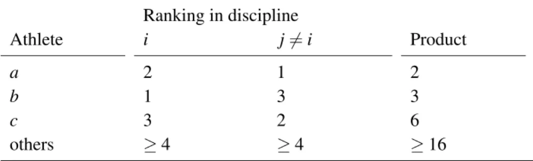
Not weakly determined: for an arbitrary discipline i ∈ N, take a profile where some athlete a∈ A comes first in all other disciplines and second in this discipline: ri(a) = 2 and rj(a) = 1
for all j ∈ N, j 6= i. If n > 2, then a is the unique winner, thus the discipline does not determine the gold. For n = 2, the profile displayed in Table 1.3 shows that i does not weakly determine the gold (we use the assumption that m ≥ 3).
Table 1.3: A profile that shows that inverse-Borda-Nash is not weakly determined for n = 2. Athlete ais the overall winner, though athlete b wins for (arbitrary) discipline i.
Ranking in discipline Athlete i j6= i Product a 2 1 2 b 1 3 3 c 3 2 6 others ≥ 4 ≥ 4 ≥ 16
1.3
Manipulation in the discipline aggregation framework
In this section we develop formal definitions of manipulation, one of which encapsulates the example given in Section 1.1. These definitions are general enough that they apply to any discipline aggregator, including the specific cases of m = 6, m = 20 and n = 3 that will be in place for sports climbing at the 2020 Olympics. Of course, we do not cover all possible types of manipulation here.
We only consider manipulations that apply to the discipline aggregator. We are not concerned with doping, score fixing, betting, or any other of the many documented examples of foul play in sports competitions, problems that any designer of a discipline aggregator would find difficult to directly combat. A characteristic of the manipulations that we do consider is that they involve an athlete deliberately performing badly. However, we are not concerned with deliberate bad performances that cause restarts (Jimenez, 2012), or that otherwise abuse the rules internal to the competition. An example of manipulation that a scrupulous designer of discipline aggregators might be able to prevent is the following: a competitor, in the group stages of a knockout tournament, deliberately loses a match in order to face a weaker opponent in the following round. Such manipulation seems to have occurred at the 2012 Olympics (TheGuardian, 2012).10
For our purposes, a manipulating athlete changes the sincere profile, P, to some other manip-ulated profile, P′, where the only changes possible are that the manipulator is ranked worse in one or more of the disciplines. The manipulator only has incentive to make the changes if
10Another example that fits our definitions of manipulation is the phenomenon of “team orders” in Formula
the manipulated profile P′is more desirable to her than the sincere profile. So, for manipula-tion to be a problem, two condimanipula-tions need to be fulfilled: the athlete needs to be able to force the manipulated profile P′to occur, and they need to prefer it to the real profile P. These two conditions involve a few assumptions.
We assume that the athlete knows what the results would be if everyone were to perform to their best abilities—that is, the athlete knows what the sincere profile is. This may be justified by the claim that the athlete knows roughly how good the other athletes are, especially in the specific case of the final round of the sports climbing event where the first round can be taken as a proxy. Relatedly, we assume that no other athletes will manipulate, so that the sincere profile would indeed be the result if the manipulator did not manipulate. This is a simplifying assumption: we have to start somewhere, and we don’t want to start by considering levels of rationality.11 We also assume that the athlete can precisely control how much worse they perform. In general, this is perhaps unrealistic, though there are specific cases where this is extremely reasonable: the speed competition runs head-to-head, so for certain configurations of profiles it would be easy to perform a specific manipulation that results in a specific ranking. Altogether, our assumptions are no stronger than those of what is probably the most important theorem concerning manipulation in social choice theory: the Gibbard-Satterthwaite Theorem.
We write the condition restricting which profiles an athlete can manipulate to—given a start-ing sincere profile—as follows. From a sincere profile P, a profile P′is a possible manipula-tion by athlete a if12
(1.i) for all i ∈ N, x ∈ A\{a} and y ∈ A, xPiyimplies xP′iy.
This discipline manipulation condition underlies all of our following definitions of ma-nipulation. The distinct definitions of manipulation only differ in what is required for the profile P′to be preferred by a to P. The clearest reason that an athlete may prefer one profile to another is if it results in a better output ranking for the athlete herself. Supposing that a manipulates from P to P′, and writing R = F(P) and R′= F(P′), this condition requires that
rR′(a) < rR(a).
We refer to this as an egoistic manipulation.13 Egoistic manipulation is impossible under in-verse Borda-Nash: if an athlete worsens their ranking in one or more disciplines, she receives a strictly larger product score, whereas all other athletes receive at most the same product
11Our analysis can be considered decision theoretic as opposed to game theoretic.
12Note that we do not consider the possibility that two or more agents manipulate together. In such a case, a
manipulator may be able to rank higher than in the sincere profile.
13Egoistic manipulation can be compared to traditional definitions of monotonicity. However, note that the
score as before, thus any athletes that she was weakly defeated by according to the sincere profile will still weakly defeat her according to the non-sincere profile. Other rules, however, do permit egoistic manipulation.14
In contrast to egoistic manipulation, where an athlete improves their own output ranking, an athlete may manipulate in order to improve the output ranking of some other athlete. One may suppose that this other athlete is a teammate, friend, or comes from the same country. Given profiles and P and P′as in the discipline manipulation condition, an athlete a manipulates for athlete b if
(1.ii) rR′(b) < rR(b).
We call this altruistic manipulation.15 Technically, this definition includes egoistic manip-ulation as the special case when a = b. Of course, if a 6= b, an altruistic manipmanip-ulation may not result in a more desirable outcome for the manipulating athlete. We now give two different, but not necessarily incompatible, reasons why an altruistic manipulation may be desirable for the manipulating athlete, the first of which comes in a strong and weak version.
The first reason seems at first sight obvious: if the altruistic manipulation involves no sacri-fice on the part of the manipulator a. This seemingly amounts to the condition
(1.iii) rR′(a) ≤ rR(a).
We will call such altruistic manipulations without sacrifice. However, there is a slight sub-tlety involved here; although we have said that the output ranks are the most important thing for discipline aggregation, pairwise comparisons may still have a secondary importance: it seems preferable to win the gold uniquely than to share it with other athletes. Even if an athlete can manipulate without sacrifice, they may nonetheless not want to do so because they end up sharing their rank with more athletes than before. The following condition rules out this possibility,
(1.iv)
{x ∈ A : xR′a}
≥ |{x ∈ A : xRa}| ,
if this is satisfied as well as (1.iii) above we say that a manipulation is completely without sacrifice. Because it occurs in fewer profiles, manipulation completely without sacrifice is easier to prevent than manipulation (just) without sacrifice.
The example of manipulation given in Section 1.1 is not a manipulation without sacrifice. The idea instead is that the manipulating athlete recognises that she probably won’t get a
14Cf. non-monotonic binary trees, Chapter 2.
15One might also consider the possibility of spiteful manipulation, whereby an athlete manipulates in order
higher ranking than her teammate, but can nonetheless manipulate to aid her teammate. The condition that ensures this is the following
(1.v) rR′(b) < rR(a).
We give manipulation of this type the name spoiler, this refers to the fact that a poorly ranked athlete spoils the fair result concerning other, better ranked, athletes. The condition ensures that b performs better than a would have done.16
We now formally state the full definitions of the two main types of manipulation that we are interested in, the first of which splits into its strong and a weak versions.
Definition 1.2(Non-sacrificial manipulation). Let F (PPP) = R and F (PPP′) = R′, and a, b ∈ A. Competitor a can manipulate without sacrifice, for competitor b, from the profile PPPto the profile PPP′if
(1.i) for all i ∈ N, x ∈ A\{a} and y ∈ A, xPiyimplies xP′iy (1.ii) rR′(b) < rR(b)
(1.iii) rR′(a) ≤ rR(a).
Such a manipulation is completely without sacrifice if it also satisfies (1.iv) |{x ∈ A : xR′a}| ≥ |{x ∈ A : xRa}|.
Definition 1.3(Spoiler manipulation). Let F (PPP) = R and F (PPP′) = R′, and a, b ∈ A. Athlete acan spoil, for athlete b, from the profile PPPto the profile PPP′if
(1.i) for all i ∈ N, x ∈ A\{a} and y ∈ A, xPiyimplies xP′iy (1.ii) rR′(b) < rR(b)
(1.v) rR′(b) < rR(a).
When both the athlete b and the profiles are implicit and need not be specified, we will say simply that athlete a spoils.
Two final remarks on our definitions of manipulation: first, for some pairs of profiles these definitions overlap; second, they do not cover all conceivable manipulations of the discipline aggregator. In particular, there is the example of altruistic manipulation in the first round of the sports climbing event: here, the desirable outcome is that the manipulator and their target are both ranked better than seventh (and not tied if ranked sixth).
16Manipulation without sacrifice and spoiler manipulation amount to the egoistic case if we set a = b, but
manipulation completely without sacrifice does not; in fact there are cases of egoistic manipulation that are not cases of manipulation completely without sacrifice.
1.4
The likelihood of undesirable profiles: simulation
re-sults
At the time of typing, the combined format for sports climbing has not been used in many real-life events. We can, however, generate many possible outcomes for events and see what one might expect. Such simulations methods have a long history in social choice theory, where large scale data concerning individuals’ preferences has not always been readily avail-able. We consider the results of such simulations in this section. In short, our simulations suggest that for inverse-Borda-Nash, although ties are unlikely to be a problem, potential for manipulation occurs with a high probability.
We generated profiles with six athletes and three disciplines, the same numbers as in the final round of the Olympics sports climbing competition. The generated profiles form three groups: in the first group, for each discipline every possible strict linear order is equally likely—profiles are drawn from the impartial culture. For profiles in the second group there is a positive correlation in an athlete’s results across the three disciplines. In the final group there is positive correlation between two disciplines and negative correlation with the third. This third culture conforms best to our actual expectations for the competition because the two disciplines of bouldering and lead climbing have an intersection of athletes at the top level, whereas top level speed climbers do not typically compete in the other disciplines. For a profile based on the impartial culture we independently select three strict linear orders, each uniformly at random from the set of all possible linear orders. Our positively correlated culture uses the Plackett-Luce (1975; 1959) model17 with initial odds
21: 22: 23: 24: 25: 26.
Label the athletes as aj for j ∈ {1, 2, 3, 4, 5, 6}. Writing t = ∑6i=1i2, each athlete aj has a pj = j2/t probability of being ranked first. The idea is that the initial odds also represent the strengths of the athletes; in particular, we suppose that each athlete is two times stronger than her closest competitor. Given that the athletes in a set B defeat the athletes in A\B, the probabilities that determine the winners within A\B should only depend upon the relative strengths of the athletes within A\B. So if athlete ak, k 6= j ranks first, then ajhas a
j2 t− k2 =
pj 1 − pk
probability of being ranked second. If akranks first and alranks second, l 6= j, l 6= k, then aj has a
j2 t− k2− l2 =
pj 1 − pk− pl
Table 1.4: The number of randomly generated profiles that involved ties, were subject to spoiler ma-nipulation, were subject to manipulation without sacrifice, were subject to manipulation completely without sacrifice, and that were subject to any of these three types of manipulation. 100,000 six agent profiles were generated for each culture. A profile was considered subject to manipulation if any of three disjoint random pairs of agents could manipulate.
Culture Ties Spoiler
manipulation Without sacrifice Strict without sacrifice Any manipulation Impartial 632 37,730 47,807 47,326 59,660 Positive correlation 779 13,792 43,723 41,597 46,964 Negative correlation 526 44,826 48,741 48,350 63,151
probability of being ranked third. The positive correlation arises because we suppose that the athletes have the same strengths for each discipline; a profile consists of three independently generated strict linear orders using the same initial odds. A negatively correlated profile is created by taking a positively correlated profile and reversing the strict linear order of the last discipline.18
We randomly generated 100,000 profiles of each type. A profile counts as tied if at least one tie occurs at any ranking level—we do not count the number of distinct ties nor how many athletes are involved in each tie. To count manipulations, we first randomly pair the athletes into three disjoint pairs. A profile counts as manipulable if at least one of the pairs can manipulate. We perform the count separately for spoiler manipulation, manipulation without sacrifice, manipulation completely without sacrifice, and for any of these types of manipulation. The results are presented in Table 1.4.
According to our simulations, it is very unlikely that there will be a tie at any level of the output complete preorder in the final round of the competition. We also ran simulations for twenty athlete profiles obtaining similar results.19 This strongly suggests that a tie in the actual competition is very unlikely to occur: note that each of our models exhibits a
18The associated culture best represents our, somewhat naive, expectations for the competition—we expect
lead climbing and bouldering to be positively correlated with each other and negatively correlated with speed climbing.
19For profiles with twenty athletes, of the 100,000 profiles we generated for each culture, 208 profiles had
ties for the impartial culture, 1108 profiles had ties for the positively correlated culture, and only 92 profiles had ties for the negatively correlated culture that conforms best to our expectations for the actual competition.
high degree of symmetry; and such symmetries are intuitively more likely to lead to tied situations. Indeed, it has been shown that the impartial culture maximises the probability for majority cycles (Tsetlin et al., 2003), one of the necessary conditions for a tie. However, from our simulations we see more ties for the positively correlated culture; we conjecture that this is because two opposing criteria need to be fulfilled for there to be a tie: there need to be majority cycles, but these must occur among athletes with the same scores. Regardless, the incidence of ties is low even for the positive culture. Of the three cultures, we see fewest ties with the negatively correlated culture which best represents our expectations for the competition.
In contrast to the low incidence of ties, there does seem to be a high potential for manip-ulation, of both kinds. For each culture approximately half the profiles are manipulable.20 We make two further observations: first, the incidence of manipulation without sacrifice that is not also completely without sacrifice is very small—the value obtained when subtracting the value of column five from the value of column four. A loose interpretation is that for inverse-Borda-Nash there is not much difference between the stronger and weaker versions of the without sacrifice property. Second, spoiler manipulation seems less likely under the positively correlated culture. An intuitive explanation for the lower incidence of spoiler ma-nipulation for the positively correlated culture is the following: for this culture it is more likely that one athlete in a pair will always be ranked above their teammate, in which case the worse ranked athlete cannot spoil. Nevertheless, even for the positive culture there is a non-negligible potential for spoiler manipulation (more than 10% of the generated profiles).
1.5
Impossibilities that suggest a trade-off between
deci-siveness and manipulability: axiomatic results
In this section we investigate the general theoretical properties of discipline aggregators. Our investigation leads to the introduction of decisiveness as a desirable condition.
Inverse-Borda-Nash is manipulable. However, this doesn’t mean that a better discipline ag-gregator exists. Our first result of this section is the following: one cannot prevent both kinds of manipulation without violating a desirable condition. This is an impossibility result in the classical sense. Apart from the conditions concerning manipulation, the result uses only the
20We also tested profiles with twenty athletes for manipulation. Each culture resulted in higher counts of
potential manipulation than in the six athlete case. Of course, to fully address the issue of manipulation in the qualification round would require other modifications: here a manipulation is desirable if and only if it moves the target athlete below the sixth place threshold; it can also be noted that we no longer have an argument for why the non-manipulated profile is common knowledge.
weakest of our conditions; in particular, it does not rely upon the relatively strong condi-tions of athlete-neutrality and discipline-neutrality, and uses the weaker “not determined” condition as opposed to “not weakly determined”. It thus shows that almost any reasonable discipline aggregator must allow for some kind of manipulation, some of the time.
Theorem 1.4. No discipline aggregator prevents spoiler manipulation, prevents manipula-tion without sacrifice, satisfies the clear winner condimanipula-tion and is not determined.
Proof. We proceed by showing that if both types of manipulation are prevented and the clear winner condition is satisfied then there a determined discipline, that is, a discipline i ∈ N such that, for a ∈ A such that ri(a) = 1, aPx for all x 6= a. The proof follows the structure of the proof of Arrow’s theorem by Reny (2001).
Take an arbitrary discipline aggregator F that prevents spoiler manipulation and manipu-lation without sacrifice and that satisfies the clear winner condition. Consider any profile where a comes first in all disciplines and b comes last. By the clear winner condition a must be ranked first and b last. We express this fact as in the Figure 1.2.
N a | b 7→ a | b
Figure 1.2: A profile where a always comes first and b last, and the corresponding output.
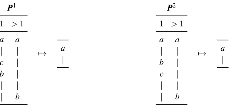
Now consider moving b up in the first discipline. So long as b does not cross above a, a must still be uniquely ranked first, as otherwise the agent c that b becomes ranked above can spoil for the new winner from PPP1 to PPP2. Note that this argument does not rely on the fact that a wins in all disciplines.
P P P1 1 > 1 a a | | c | b | | | | b 7→ a | P P P2 1 > 1 a a | | b | c | | | | b 7→ a |
Figure 1.3: A profile PPP1for which the position of b is changed, but not with respect to the unique winner a, leading to another profile PPP2for which a is still the unique winner.
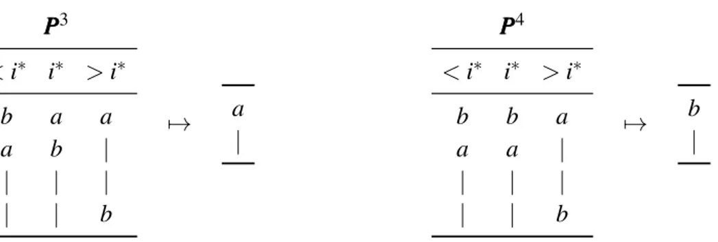
X. In the second case there is some x ∈ X, x 6= a. If we continue to successively rank b first for the remaining disciplines, then at some point b must become the unique winner by the clear winner condition—in particular when b is ranked first in all disciplines: thus the second disjunct of the previous sentence must be fulfilled at some point; there must be some profile which outputs a top, but moving b above a gives some other set of winners X. Label the discipline for which this happens i∗, and label the respective profiles as PPP3 and PPP4. Note that in PPP3athlete b has been moved up to be directly below a, the same argument as above implies that a is still the winner in the output.
PPP3 < i∗ i∗ > i∗ b a a a b | | | | | | b 7→ a | PPP4 < i∗ i∗ > i∗ b b a a a | | | | | | b 7→ b |
Figure 1.4: A critical profile PPP3 and discipline i∗ such that if athlete b is ranked above athlete a to
create PPP4, then athlete b becomes the unique winner.
We know that a /∈ X, otherwise a could spoil without sacrifice for x from PPP3 to PPP4. This implies that b ∈ X, as otherwise b could spoil for a from PPP4to PPP3. This implies that x /∈ X for x 6= a, b, as otherwise b could manipulate without sacrifice for x from the profile where b is the unique winner.
In PPP4we can move a down in the profile without changing the output winner b (otherwise a could spoil), we display this as PPP5. Also consider the profile PPP6created from PPP5by moving aup one place in discipline i∗.
PPP5 < i∗ i∗ > i∗ b b | | a | | | a a | b 7→ b | PPP6 < i∗ i∗ > i∗ b a | | b | | | a a | b 7→ a |
Figure 1.5: Profiles showing that i∗plays an important role for whether or not athlete a wins in the
output.
We claim that a must the unique winner in PPP6. First, note that if neither a nor b were ranked first for PPP6, then a can spoil for b from PPP6to PPP5. If b is ranked first but not uniquely ranked
first, then b can spoil without sacrifice from PPP5 to PPP6. If b is uniquely ranked first, then at some point in stepwise changes from PPP6 to PPP3 some other athlete must perform a spoiler manipulation. Thus as b is not ranked first a is amongst the winners. If a were not unique, a could spoil without sacrifice from PPP3to PPP6.
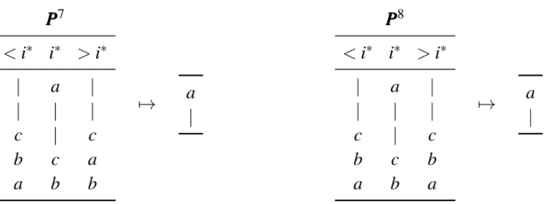
Take some third alternative c 6= a, b. The profile PPP7 is obtained from PPP6by moving b and c down in the profile. Here the unique winner is still a, as otherwise b or c could spoil. Create PPP8by moving a to be ranked last in all disciplines except i∗.
P PP7 < i∗ i∗ > i∗ | a | | | | c | c b c a a b b 7→ a | P PP8 < i∗ i∗ > i∗ | a | | | | c | c b c b a b a 7→ a |
Figure 1.6:Profiles for which a is ranked first in i∗, for which a must also be the winner in the output.
In the profile PPP8, alternative c is a clear winner over b, so b cannot be ranked first. If a were not ranked first then b could spoil for a from PPP8 to PPP7. If any other athlete is ranked first, then a can manipulate without sacrifice from PPP7to PPP8. Thus a must be the unique winner in PPP8.
In general, for any profile where a wins in discipline i∗, a must be uniquely ranked first in the output, as otherwise there would be some chain of changes from PPP8to the profile in question, one of which would be a spoiler manipulation for the new winning athlete. As a was chosen arbitrarily, for each alternative x there is a discipline ix such that whenever x wins in ix, x must be uniquely ranked first. As two alternatives x and y cannot both be ranked first, ix= iy for all x, y ∈ A, thus i∗determines the gold.
The proof of Theorem 1.4 closely follows that of Reny (2001), who presents Arrow’s impos-sibility and the Gibbard-Satterthwaite theorem side by side. Although we consider manipu-lation, the result is, in terms of its formal shape, closer to the presentation of Arrow’s result than to that of the Gibbard-Satterthwaite result. Requiring the impossibility of both forms of manipulation takes the place of binary independence, though this requirement does not imply binary independence.21 Consider the discipline aggregator that returns the total pre-order where a is ranked uniquely first and all other alternatives jointly second if a is first in
21By binary independence we mean the specific version of Arrow’s independence of irrelevant alternatives
that requires of a social welfare function F that, for all pairs {a, b} ⊆ A, for any two profiles RRR, RRR′such that for all i ∈ N xRiy⇔ xR′iy, xF(RRR)y ⇔ xF(RRR′)y (note that this definition works only because R, R′, F(RRR) and F(RRR′)
all disciplines, and a is ranked second and all other alternatives jointly first otherwise; this violates binary independence but prevents both kinds of manipulation. The no-manipulation requirement is closer to Condorcet independence of irrelevant alternatives (Yu, 2015). This means that our impossibility is not simply a corollary of Arrow’s theorem.
Theorem 1.4 is tight for the four conditions, in the sense if any one is removed there is a discipline-aggregator that satisfies the other three. Dictatorships, for which the ranking of a single discipline is copied, are determined but satisfy the other three conditions. Constant functions violate only the clear winner condition (except the function that always ranks every athlete first, which is also weakly determined). We define a function below that we call iterative first place elimination that only allows manipulation without sacrifice. Before this, we describe a function that only allows spoiler manipulation: this proceeds sequentially, at stage t, remove the athlete who is ranked last in discipline t modulo n, and rank this athlete below the other athletes remaining in the profile.22 Arguably the best exposition of this process is given by the example in Table 1.5. Formally, we define iterative successive last removal, isr : L∗(A)N→ W(A) as follows. For an arbitrary profile PPP, let lose
t(PPP) = {a ∈ A : rt(a) is maximal}. Let PPP1= PPP, and for t ≥ 1 recursively define PPPt+1 as the restriction of P
PPt to A\losetmod n(PPPt). Writing P = isr(PPP), for x, y ∈ A, define xRy if and only if there are integers s,t ≤ m such that s ≥ t and x ∈ losesmod n(PPPs) and y ∈ losetmod n(PPPt).
Proposition 1.5. Iterative successive last removal prevents manipulation without sacrifice, satisfies the clear winner condition, is not weakly determined and satisfies athlete-neutrality. Proof. Prevents manipulation without sacrifice: suppose an athlete “manipulates” by per-forming worse in a profile but also that she does not get a worse output ranking. Thus she is removed at the same point t and has output rank m − t + 1. Clearly, all the partial profiles after this point will be the same as in the non-manipulated case. As she was not removed before t, this means that for all the partial profiles at stage s < t she was not ranked last in discipline s modulo n, this means that she did not change the athlete who was ranked last in this discipline, thus the loser at this stage will be the same.
The clear winner condition: if a is better than b in all disciplines then a cannot be removed before b.
Not weakly determined: for disciplines i 6= 1, consider the profile where the athlete ranked first in i is ranked last in 1. For discipline 1 consider the profile where the athlete ranked first in 1 is ranked second last in 2.
We cannot satisfy all our properties simultaneously. However, if we strengthen manipulation without sacrifice to manipulation completely without sacrifice there are functions that work.
Table 1.5: The process of iterative successive last removal applied to the final round given the results of Table 1.1, supposing that Faye was eliminated by the external tie-breaker and the remaining athletes perform as in the first round.
Ranking Speed Bouldering Lead Final ranking
1st Barbara Dorothy Chloe
2nd Emma Grace Emma
3rd Alice Alice Dorothy
4th Chloe Barbara Grace
5th Grace Emma Barbara
6th Dorothy Chloe Alice
1st Barbara Grace Chloe
2nd Emma Alice Emma
3rd Alice Barbara Grace
4th Chloe Emma Barbara
5th Grace Chloe Alice
6th Dorothy
1st Barbara Grace Emma
2nd Emma Alice Grace
3rd Alice Barbara Barbara
4th Grace Emma Alice
5th Chloe
6th Dorothy
1st Barbara Grace Emma
2nd Emma Barbara Grace
3rd Grace Emma Barbara
4th Alice
5th Chloe
6th Dorothy
1st Barbara Barbara Emma
2nd Emma Emma Barbara
3rd Grace
4th Alice
5th Chloe
6th Dorothy
1st Barbara Barbara Barbara Barbara
2nd Emma
3rd Grace
4th Alice
5th Chloe
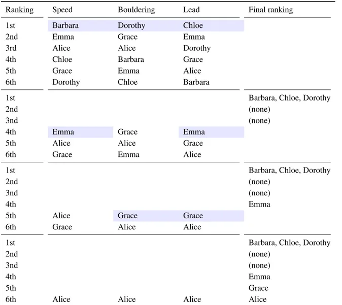
Table 1.6:The process of iterative first place elimination applied to the final round given the results of Table 1.1, supposing that Faye was eliminated by the external tie-breaker and the remaining athletes perform as in the first round.
Ranking Speed Bouldering Lead Final ranking
1st Barbara Dorothy Chloe
2nd Emma Grace Emma
3rd Alice Alice Dorothy
4th Chloe Barbara Grace
5th Grace Emma Alice
6th Dorothy Chloe Barbara
1st Barbara, Chloe, Dorothy
2nd (none)
3nd (none)
4th Emma Grace Emma
5th Alice Alice Grace
6th Grace Emma Alice
1st Barbara, Chloe, Dorothy
2nd (none)
3nd (none)
4th Emma
5th Alice Grace Grace
6th Grace Alice Alice
1st Barbara, Chloe, Dorothy
2nd (none)
3nd (none)
4th Emma
5th Grace