Nonlinear reduced models for state and parameter estimation
Albert Cohen, Wolfgang Dahmen, Olga Mula and James Nichols∗ September 8, 2020
Abstract
State estimation aims at approximately reconstructing the solution u to a parametrized par-tial differenpar-tial equation from m linear measurements, when the parameter vector y is unknown. Fast numerical recovery methods have been proposed in [19] based on reduced models which are linear spaces of moderate dimension n which are tailored to approximate the solution man-ifold M where the solution sits. These methods can be viewed as deterministic counterparts to Bayesian estimation approaches, and are proved to be optimal when the prior is expressed by approximability of the solution with respect to the reduced model [2]. However, they are inher-ently limited by their linear nature, which bounds from below their best possible performance by the Kolmogorov width dmpMq of the solution manifold. In this paper we propose to break this
barrier by using simple nonlinear reduced models that consist of a finite union of linear spaces Vk, each having dimension at most m and leading to different estimators u˚k. A model selection
mechanism based on minimizing the PDE residual over the parameter space is used to select from this collection the final estimator u˚. Our analysis shows that u˚ meets optimal recovery
benchmarks that are inherent to the solution manifold and not tied to its Kolmogorov width. The residual minimization procedure is computationally simple in the relevant case of affine parameter dependence in the PDE. In addition, it results in an estimator y˚
for the unknown parameter vector. In this setting, we also discuss an alternating minimization (coordinate de-scent) algorithm for joint state and parameter estimation, that potentially improves the quality of both estimators.
1
Introduction
1.1 Parametrized PDEs and inverse problems
Parametrized partial differential equations are of common used to model complex physical systems. Such equations can generally be written in abstract form as
Ppu, yq “ 0, (1.1)
where y“ py1, . . . , ydq is a vector of scalar parameters ranging in some domain Y Ă Rd. We assume
well-posedness, that is, for any yP Y the problem admits a unique solution u “ upyq in some Hilbert space V . We may therefore consider the parameter to solution map
y ÞÑ upyq, (1.2)
∗
This research was supported by the ERC Adv grant BREAD; the Emergence Project of the Paris City Council “Models and Measures”; the NSF Grant DMS ID 2012469, and by the SmartState and Williams-Hedberg Foundation.
from Y to V , which is typically nonlinear, as well as the solution manifold
M :“ tupyq : y P Y u Ă V (1.3)
that describes the collection of all admissible solutions. Throughout this paper, we assume that Y is compact in Rd and that the map (1.2) is continuous. Therefore M is a compact set of V . We sometimes refer to the solution upyq as the state of the system for the given parameter vector y.
The parameters are used to represent physical quantities such as diffusivity, viscosity, velocity, source terms, or the geometry of the physical domain in which the PDE is posed. In several relevant instances, y may be high or even countably infinite dimensional, that is, d" 1 or d “ 8.
In this paper, we are interested in inverse problems which occur when only a vector of linear measurements
z“ pz1, . . . , zmq P Rm, zi “ ℓipuq, i“ 1, . . . , m, (1.4)
is observed, where each ℓi P V1 is a known continuous linear functional on V . We also sometimes
use the notation
z“ ℓpuq, ℓ“ pℓ1, . . . , ℓmq. (1.5)
One wishes to recover from z the unknown state uP M or even the underlying parameter vector yP Y for which u “ upyq. Therefore, in an idealized setting, one partially observes the result of the composition map
yP Y ÞÑ u P M ÞÑ z P Rm. (1.6)
for the unknown y. More realistically, the measurements may be affected by additive noise
zi “ ℓipuq ` ηi, (1.7)
and the model itself might be biased, meaning that the true state u deviates from the solution manifold M by some amount. Thus, two types of inverse problems may be considered:
(i) State estimation: recover an approximation u˚ of the state u from the observation z “ ℓpuq. This is a linear inverse problem, in which the prior information on u is given by the manifold Mwhich has a complex geometry and is not explicitly known.
(ii) Parameter estimation: recover an approximation y˚ of the parameter y from the observation z“ ℓpuq when u “ upyq. This is a nonlinear inverse problem, for which the prior information available on y is given by the domain Y .
These problems become severely ill-posed when y has dimension d ą m. For this reason, they are often addressed through Bayesian approaches [17,25]: a prior probability distribution Py being
assumed on y P Y (thus inducing a push forward distribution Pu for u P M), the objective is
to understand the posterior distributions of y or u conditionned by the observations z in order to compute plausible solutions y˚or u˚under such probabilistic priors. The accuracy of these solutions should therefore be assessed in some average sense.
In this paper, we do not follow this avenue: the only priors made on y and u are their membership to Y and M. We are interested in developping practical estimation methods that offer uniform recovery guarantees under such deterministic priors in the form of upper bounds on the worst case error for the estimators over all y P Y or u P M. We also aim to understand whether our error bounds are optimal in some sense. Our primary focus will actually be on state estimation (i). Nevertheless we present in §4 several implications on parameter estimation (ii), which to our knowledge are new. For state estimation, error bounds have recently been established for a class of methods based on linear reduced modeling, as we recall next.
1.2 Reduced models: the PBDW method
In several relevant instances, the particular parametrized PDE structure allows one to construct linear spaces Vnof moderate dimension n that are specifically tailored to the approximation of the
solution manifold M, in the sense that
distpM, Vnq “ max uPMvPVminn
}u ´ v} ď εn, (1.8)
where εn is a certified bound that decays with n significanly faster than when using for Vn classical
approximation spaces such as finite elements, algebraic or trigonometric polynomials, or spline functions of dimension n. Throughout this paper
} ¨ } “ } ¨ }V, (1.9)
denotes the norm of the Hilbert space V . The natural benchmark for such approximation spaces is the Kolmogorov n-width
dnpMq :“ min
dimpEq“ndistpM, Eq. (1.10)
The space Enthat achieves the above minimum is thus the best possible reduced model for
approx-imating all of M, however it is computationally out of reach.
One instance of computational reduced model spaces is generated by sparse polynomial approx-imations of the form
unpyq “ ÿ νPΛn uνyν, yν :“ ź jě1 yνj j , (1.11)
where Λn is a conveniently chosen set of multi-indices such that #pΛnq “ n. Such approximations
can be derived, for example, by best n-term truncations of infinite Taylor or orthogonal polynomial expansions. We refer to [11,12] where convergence estimates of the form
sup
yPY
}upyq ´ unpyq} ď Cn´s, (1.12)
are established for some s ą 0 even when d “ 8. Therefore, the space Vn :“ spantuν : ν P Λnu
approximates the solution manifold with accuracy εn“ Cn´s.
Another instance, known as reduced basis approximation, consists of using spaces of the form
Vn:“ spantu1, . . . , unu, (1.13)
where ui “ upyiq P M are instances of solutions corresponding to a particular selection of parameter
values yi P Y [20, 23, 24]. One typical selection procedure is to pick yk such that u
k “ upykq is
furthest away from the previously constructed space Vk´1. It was proved in [1,16] that the reduced
basis spaces resulting from this greedy algorithm have near-optimal approximation property, in the sense that if dnpMq has a certain polynomial or exponential rate of decay as n Ñ 8, then the same
rate is achieved by distpM, Vnq.
In both cases, these reduced models come in the form of a hierarchy pVnqně1, with decreasing
error bounds pεnqně1, where n corresponds to the level of truncation in the first case and the step
of the greedy algorithm in the second case. Given a reduced model Vn, one way of tackling the
state estimation problem is to replace the complex solution manifold M by the simpler prior class described by the cylinder
that contains M. The set K therefore reflects the approximability of M by Vn. This point of view
leads to the Parametrized Background Data Weak (PBDW) method introduced in [19], also termed as one space method and further analyzed in [2], that we recall below in a nutshell.
In the noiseless case, the knowledge of z “ pziqi“1,...,m is equivalent to that of the orthogonal
projection w“ PWu, where
W :“ spantω1, . . . , ωmu (1.15)
and ωiP V are the Riesz representers of the linear functionals ℓi, that is
ℓipvq “ xωi, vy, vP V. (1.16)
Thus, the data indicates that u belongs to the affine space
Vw :“ w ` WK. (1.17)
Combining this information with the prior class K, the unknown state thus belongs to the ellipsoid
Kw:“ K X Vw“ tv P K : PWv “ wu. (1.18)
For this posterior class Kw, the optimal recovery estimator u˚ that minimizes the worst case error
maxuPKw}u ´ u˚} is therefore the center of the ellipsoid, which is equivalently given by
u˚ “ u˚pwq :“ argmint}v ´ PVnv} : PWv“ wu. (1.19)
It can be computed from the data w in an elementary manner by solving a finite set of linear equations. The worst case performance for this estimator, both over K and Kw, for any w, is thus
given by the half-diameter of the ellipsoid which is the product of the width εnof K by the quantity
µn“ µpVn, Wq :“ max vPVn
}v} }PWv}
, (1.20)
which is the inverse of the cosine of the angle between Vn and W . For n ě 1, this quantity can
be computed as the inverse of the smallest singular value of the nˆ m cross-Gramian matrix with entries xφi, ψjy between any pair of orthonormal bases pφiqi“1,...,n and pψjqj“1,...,m of Vn and W ,
respectively. It is readily seen that one also has µn“ max wPWK }w} }PVK nw} , (1.21)
allowing us to extend the above definition to the case of the zero-dimensional space Vn “ t0u for
which µpt0u, W q “ 1.
Since MĂ K, the worst case error bound over M of the estimator, defined as Ewc:“ max
uPM}u ´ u ˚pP
Wuq} (1.22)
satisfies the error bound
Ewc“ max uPM}u ´ u ˚pP Wuq} ď max uPK }u ´ u ˚pP Wuq}“ µnεn. (1.23)
Remark 1.1 The estimation map w ÞÑ u˚pwq is linear with norm µn and does not depend on εn. It thus satisfies, for any individual uP V and η P W ,
}u ´ u˚pPWu` ηq} ď µnpdistpu, Vnq ` }η}q, (1.24)
We may therefore account for an additional measurement noise and model bias: if the observation is w“ PWu`η with }η} ď εnoise, and if the true states do not lie in M but satisfy distpu, Mq ď εmodel,
the guaranteed error bound (1.23) should be modified into
}u ´ u˚pwq} ď µnpεn` εnoise` εmodelq. (1.25)
In practice, the noise component η P W typically results from a noise vector η P Rm affecting the
observation z according to z“ ℓpuq ` η. Assuming a bound }η}2ď εnoise where} ¨ }2 is the Euclidean
norm in Rm, we thus receive the above error bound with ε
noise :“ }M }εnoise, where M P Rmˆm
is the matrix that transforms the representer basis ω “ tω1, . . . , ωmu into an orthonormal basis
ψ“ tψ1, . . . , ψmu of W .
Remark 1.2 To bring out the essential mechanisms, we have idealized (and technically simplified) the description of the PBDW method by ommitting certain discretization aspects that are unavoidable in computational practice and should be accounted for. To start with, the snapshots ui (or the
polynomial coefficients uν) that span the reduced basis spaces Vn cannot be computed exactly, but
only up to some tolerance by a numerical solver. One typical instance is the finite element method, which yields an approximate parameter to solution map
yÞÑ uhpyq P Vh, (1.26)
where Vh is a reference finite element space ensuring a prescribed accuracy
}upyq ´ uhpyq} ď εh, yP Y. (1.27)
The computable states are therefore elements of the perturbed manifold
Mh :“ tuhpyq : y P Y u. (1.28)
The reduced model spaces Vn are low dimensional subspaces of Vh, and with certified accuracy
distpMh, Vnq ď εn. (1.29)
The true states do not belong to Mh and this deviation can therefore be interpreted as a model bias
in the sense of the previous remark with εmodel “ εh. The application of the PDBW also requires
the introduction of the Riesz lifts ωi in order to define the measurement space W . Since we operate
in the space Vh, these can be defined as elements of this space satisfying
xωi, vy “ ℓipvq, vP Vh, (1.30)
thus resulting in a measurement space W Ă Vh. For example, if V is the Sobolev spaces H01pΩq for
some domain Ω and Vh is a finite element subspace, the Riesz lifts are the unique solutions to the
Galerkin problem ż
Ω
and can be identified by solving nhˆ nh linear systems. Measuring accuracy in V , i.e., in a metric
dictated by the continuous PDE model, the idealization, to be largely maintained in what follows, also helps understanding how to properly adapt the background-discretization Vh to the overall achievable
estimation accuracy. Other computational issues involving the space Vh will be discussed in §3.4.
Note that µn ě 1 increases with n and that its finiteness imposes that dimpVnq ď dimpW q,
that is mě n. Therefore, one natural way to decide which space Vn to use is to take the value of
nP t0, . . . , mu that minimizes the bound µnεn. This choice is somehow crude since it might not be
the value of n that minimizes the true reconstruction error for a given uP M, and for this reason it was referred to as a poor man algorithm in [1].
The PBDW approach to state estimation can be improved in various ways:
• One variant that is relevant to the present work is to use reduced models of affine form
Vn“ un` Vn, (1.32)
where Vn is a linear space and u is a given offset. The optimal recovery estimator is again
defined by the minimization property (1.19). Its computation amounts to the same type of linear systems and the reconstruction map w ÞÑ u˚pwq is now affine. The error bound (1.23) remains valid with µn “ µpVn, Wq and εn a bound for distpM, Vnq. Note that εn is
also a bound for the distance of M to the linear space Vn`1 :“ Vn ‘ Run of dimension
n` 1. However, using instead this linear space, could result in a stability constant µn`1 “
µpVn`1, Wq that is much larger than µn, in particular, when the offset unis close to WK.
• Another variant proposed in [10] consists in using a large set TN “ tui “ upyiq : i “ 1, . . . , N u
of precomputed solutions in order to train the reconstruction maps wÞÑ u˚pwq by minimizing
the least-square fit řNi“1}ui ´ u˚pPWuiq}2 over all linear or affine map, which amounts to
optimizing the choice of the space Vn in the PBDW method.
• Conversely, for a given reduced basis space Vn, it is also possible to optimize the choice of
linear functionalspℓ1, . . . , ℓmq giving rise to the data, among a dictionary D that represent a
set of admissible measurement devices. The objective is to minimize the stability constant µpVn, Wq for the resulting space W , see in particular [3] where a greedy algorithm is proposed
for selecting the ℓi. We do not take this view in the present paper and think of the space W
as fixed once and for all: the measurement devices are given to us and cannot be modified.
1.3 Objective and outline
The simplicity of the PBDW method and its above variants come together with a fundamental limitation of its performance: since the map w ÞÑ u˚pwq is linear or affine, the reconstruction
necessarily belongs to an m or m` 1 dimensional space, and thefore the worst case performance is necessarily bounded from below by the Kolmogorov width dmpMq or dm`1pMq. In view of
this limitation, one principle objective of the present work is to develop nonlinear state estimation techniques which provably overcome the bottleneck of the Kolmogorov width dmpMq.
In §2, we introduce various benchmark quantities that describe the best possible performance of a recovery map in a worst case sense. We first consider an idealized setting where the state u is assumed to exactly satisfy the theoretical model described by the parametric PDE, that is uP M.
Then we introduce similar benchmarks quantities in the presence of model bias and measurement noise. All these quantities can be substantially smaller than dmpMq.
In §3, we discuss a nonlinear recovery method, based on a family of affine reduced models pVkqk“1,...,K, where each Vk has dimension nk ď m and serves as a local approximations to a
portion Mk of the solution manifold. Applying the PBDW method with each such space, results
in a collection of state estimators u˚k. The value k for which the true state u belongs to Mk
being unknown, we introduce a model selection procedure in order to pick a value k˚, and define the resulting estimator u˚ “ u˚
k˚. We show that this estimator has performance comparable to
the benchmark introduced in §2. Such performances cannot be achieved by the standard PBDW method due to the above described limitations.
Model selection is a classical topic of mathematical statistics [22], with representative techniques such as complexity penalization or cross-validation in which the data are used to select a proper model. Our approach differs from these techniques in that it exploits (in the spirit of data as-similation) the PDE model which is available to us, by evaluating the distance to the manifold
distpv, Mq “ min
yPY }v ´ upyq}, (1.33)
of the different estimators v “ u˚k for k “ 1, . . . , K, and picking the value k˚ that minimizes it. In practice, the quantity (1.33) cannot be exactly computed and we instead rely on a computable surrogate quantity Spv, Mq expressed in terms of the residual to the PDE, see § 3.4.
One typical instance where such a surrogate is available is when (1.1) has the form of a linear operator equation
Apyqu “ f pyq, (1.34)
where Apyq is boundedly invertible from V to V1, or more generally, from V Ñ Z1 for a test space
Z different from V , uniformly over yP Y . Then Spv, Mq is obtained by minimizing the residual
Rpv, yq “ }Apyqv ` f pyq}Z1, (1.35)
over y P Y . This task itself is greatly facilitated in the case where the operators Apyq and source terms fpyq have affine dependence in y. One relevant example that has been often considered in the literature is the second order elliptic diffusion equation with affine diffusion coefficient,
´divpa∇uq “ f pyq, a“ apyq “ a `
d
ÿ
j“1
yjψj. (1.36)
In §4, we discuss the more direct approach for both state and parameter estimation based on minimizing Rpv, yq over both y P Y and v P w ` WK. The associated alternating minimization algorithm amounts to a simple succession of quadratic problems in the particular case of linear PDE’s with affine parameter dependence. Such an algorithm is not guaranteed to converge to a global minimum (since the residual is not globally convex), and for this reason its limit may miss the optimaliy benchmark. On the other hand, using the estimator derived in §3 as a “good initialization point” to this mimimization algorithm leads to a limit state that has at least the same order of accuracy.
These various approaches are numerically tested in §5 for the elliptic equation (1.36), for both the overdetermined regime mě d, and the underdetermined regime m ă d.
2
Optimal recovery benchmarks
In this section we describe the performance of the best possible recovery map
wÞÑ u˚pwq, (2.1)
in terms of its worst case error. We consider first the case of noiseless data and no model bias. In a subsequent step we take such perturbations into account. While these best recovery maps cannot be implemented by a simple algorithm, their performance serves as benchmark for the nonlinear state estimation algorithms discussed in the next section.
2.1 Optimal recovery for the solution manifold
In the absence of model bias and when a noiseless measurement w“ PWu is given, our knowledge
on u is that it belongs to the set
Mw:“ M X Vw. (2.2)
The best possible recovery map can be described through the following general notion.
Definition 2.1 The Chebychev ball of a bounded set S P V is the closed ball Bpv, rq of minimal radius that contains S. One denotes by v “ cenpSq the Chebychev center of S and r “ radpSq its Chebychev radius.
In particular one has
1
2diampSq ď radpSq ď diampSq, (2.3)
where diampSq :“ supt}u ´ v} : u, v P Su is the diameter of S. Therefore, the recovery map that minimizes the worst case error over Mw for any given w, and therefore over M is defined by
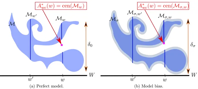
u˚pwq “ cenpMwq. (2.4)
Its worst case error is
Ewc˚ “ suptradpMwq : w P W u. (2.5)
In view of the equivalence (2.3), we can relate Ewc˚ to the quantity
δ0“ δ0pM, W q :“ suptdiampMwq : w P W u “ supt}u ´ v} : u, v P M, u ´ v P WKu, (2.6) by the equivalence 1 2δ0 ď E ˚ wc ď δ0. (2.7)
Note that injectivity of the measurement map PW over M is equivalent to δ0 “ 0. We provide in
Figure (2.1a) an illustration the above benchmark concepts.
If w“ PWufor some uP M, then any u˚ P M such that PWu˚“ w, meets the ideal benchmark
}u ´ u˚} ď δ0. Therefore, one way for finding such a u˚ would be to minimize the distance to the
manifold over all functions such that PWv“ w, that is, solve
min vPVw distpv, Mq “ min vPVw min yPY }upyq ´ v}. (2.8)
This problem is computationally out of reach since it amounts to the nested minimization of two non-convex functions in high dimension.
Computationally feasible algorithms such as the PBDW methods are based on a simplification of the manifold M which induces an approximation error. We introduce next a somewhat relaxed benchmark that takes this error into account.
(a) Perfect model. (b) Model bias.
Figure 2.1: Illustration of the optimal recovery benchmark on a manifold in the two dimensional euclidean space.
2.2 Optimal recovery under perturbations
In order to account for manifold simplification as well as model bias, for any given accucary σą 0, we introduce the σ-offset of M,
Mσ :“ tv P V : distpv, Mq ď σu “ ď
uPM
Bpu, σq. (2.9)
Likewise, we introduce the perturbed set
Mσ,w “ MσX Vw, (2.10)
which, however, still excludes uncertainties in w. Our benchmark for the worst case error is now defined as (see Figure (2.1b) for an illustration)
δσ :“ max
wPWdiampMσ,wq “ maxt}u ´ v} : u, v P Mσ, u´ v P W
Ku. (2.11)
The map σÞÑ δσ satisfies some elementary properties:
• Monotonicity and continuity: it is obviously non-decreasing
σ ď ˜σ ùñ δσ ď δσ˜. (2.12)
Simple finite dimensional examples show that this map may have jump discontinuities. Take for example a compact set M Ă R2 consisting of the two points p0, 0q and p1{2, 1q, and
W “ Re1 where e1 “ p1, 0q. Then δσ “ 2σ for 0 ď σ ď 14, while δ1
4pM, W q “ 1. Using the
compactness of M, it is possible to check that σ ÞÑ δσ is continuous from the right and in
• Bounds from below and above: for any u, vP Mσ,w, and for any ˜σ ě 0, let ˜u“ u ` ˜σg and
˜
v“ v ´ ˜σg with g “ pu ´ vq{}u ´ v}. Then, }˜u´ ˜v} “ }u ´ v} ` 2˜σ and ˜u´ ˜vP WK, which
shows that ˜u, ˜vP Mσ`˜σ,w, and
δσ`˜σ ě δσ` 2˜σ. (2.13)
In particular,
δσ ě δ0` 2σ ě 2σ. (2.14)
On the other hand, we obviously have the upper bound δσ ď diampMσq ď diampMq ` 2σ.
• The quantity
µpM, W q :“ 1 2supσą0
δσ´ δ0
σ , (2.15)
may be viewed as a general stability constant inherent to the recovery problem, similar to µpVn, Wq that is more specific to the particular PBDW method: in the special case where
M“ Vn and VnX WK “ t0u, one has δ0 “ 0 and δσ
σ “ µpVn, Wq for all σ ą 0. Note that
µpM, W q ě 1 in view of (2.14).
Regarding measurement noise, it suggests to introduce the quantity ˜
δσ :“ maxt}u ´ v} : u, v P M, }PWu´ PWv} ď σu. (2.16)
The two quantities δσ and ˜δσ are not equivalent, however one has the framing
δσ´ 2σ ď ˜δ2σ ď δσ` 2σ. (2.17)
To prove the upper inequality, we note that for any u, vP Mσ such that u´ v P WK, there exists
˜
u, ˜vP M at distance σ from u, v, respectively, and therefore such that }PWp˜u´˜vq} ď 2σ. Conversely,
for any ˜u, ˜vP M such that }PWp˜u´˜vq} ď 2σ, there exists u, v at distance σ from ˜u, ˜v, respectively,
such that u´ v P WK, which gives the lower inequality. Note that the upper inequality in (2.17) combined with (2.14) implies that ˜δ2σď 2δσ.
In the following analysis of reconstruction methods, we use the quantity δσ as a benchmark
which, in view of this last observation, also accounts for the lack of accuracy in the measurement of PWu. Our objective is therefore to design an algorithm that, for a given tolerance σ ą 0, recovers
from the measurement w“ PWu an approximation to u with accuracy comparable to δσ. Such an
algorithm requires that we are able to capture the solution manifold up to some tolerance εď σ by some reduced model.
3
Nonlinear recovery by reduced model selection
3.1 Piecewise affine reduced models
Linear or affine reduced models, as used in the PBDW algorithm, are not suitable for approximating the solution manifold when the required tolerance ε is too small. In particular, when εădmpMq one
would then need to use a linear space Vn of dimension nąm, therefore making µpVn, Wq infinite.
One way out is to replace the single space Vn by a family of affine spaces
each of them having dimension
dimpVkq “ nkď m, (3.2)
such that the manifold is well captured by the union of these spaces, in the sense that dist´M, K ď k“1 Vk ¯ ď ε (3.3)
for some prescribed tolerance εą 0. This is equivalent to saying that there exists a partition of the solution manifold M“ K ď k“1 Mk, (3.4)
such that we have local certified bounds
distpMk, Vkq ď εkď ε, k“ 1, . . . , K. (3.5)
We may thus think of the family pVkqk“1,...,K as a piecewise affine approximation to M. We stress
that, in contrast to the hierarchies pVnqn“0,...,m of reduced models discussed in §1.2, the spaces Vk
do not have dimension k and are not nested. Most importantly, K is not limited by m while each nk is.
The objective of using a piecewise reduced model in the context of state estimation is to have a joint control on the local accuracy εk as expressed by (3.5) and on the stability of the PBDW when
using any individual Vk. This means that, for some prescribed µą 1, we ask that
µk “ µpVk, Wq ď µ, k“ 1, . . . , K. (3.6)
According to (1.23), the worst case error bound over Mk when using the PBDW method with a
space Vk is given by the product µkεk. This suggests to alternatively require from the collection
pVkqk“1,...,K, that for some prescribed σ ą 0, one has
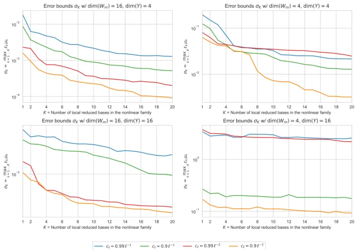
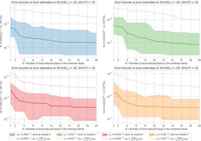
σk:“ µkεkď σ, k“ 1, . . . , K. (3.7)
This leads us to the following definitions.
Definition 3.1 The familypVkqk“1,...,K is σ-admissible if (3.7) holds. It ispε, µq-admissible if (3.5) and (3.6) are jointly satisfied.
Obviously, any pε, µq-admissible family is σ-admissible with σ :“ µε. In this sense the notion of pε, µq-admissibility is thus more restrictive than that of σ-admissibility. The benefit of the first notion is in the uniform control on the size of µ which is critical in the presence of noise, as hinted at by Remark 1.1.
If u P M is our unknown state and w “ PWu is its observation, we may apply the PBDW
method for the different Vk in the given family, which yields a corresponding family estimators
u˚k “ u˚kpwq “ argmintdistpv, Vkq : v P Vwu, k“ 1, . . . , K. (3.8)
IfpVkqk“1,...,K is σ-admissible, we find that the accuracy bound
holds whenever uP Mk.
Therefore, if in addition to the observed data w one had an oracle giving the information on which portion Mk of the manifold the unknown state sits, we could derive an estimator with worst
case error
Ewcď σ. (3.10)
This information is, however, not available and such a worst case error estimate cannot be hoped for, even with an additional multiplicative constant. Indeed, as we shall see below, σ can be fixed arbitrarily small by the user when building the family pVkqk“1,...,K, while we know from §2.1 that
the worst case error is bounded from below by E˚
wc ě 12δ0 which could be non-zero. We will thus
need to replace the ideal choice of k by a model selection procedure only based on the data w, that is, a map
wÞÑ k˚pwq, (3.11)
leading to a choice of estimator u˚ “ u˚
k˚. We shall prove further that such an estimator is able to
achieve the accuracy
Ewcď δσ, (3.12)
that is, the benchmark introduced in §2.2. Before discussing this model selection, we discuss the existence and construction of σ-admissible or pε, µq-admissible families.
3.2 Constructing admissible reduced model families
For any arbitrary choice of ε ą 0 and µ ě 1, the existence of an pε, µq-admissible family results from the following observation: since the manifold M is a compact set of V , there exists a finite ε-cover of M, that is, a family u1, . . . , uK P V such that
MĂ
K
ď
k“1
Bpuk, εq, (3.13)
or equivalently, for all v P M, there exists a k such that }v ´ uk} ď ε. With such an ε cover, we
consider the family of trivial affine spaces defined by
Vk“ tuku “ uk` Vk, Vk“ t0u, (3.14)
thus with nk“ 0 for all k. The covering property implies that (3.5) holds. On the other hand, for
the 0 dimensional space, one has
µpt0u, W q “ 1, (3.15)
and therefore (3.6) also holds. The family pVkqk“1,...,K is therefore pε, µq-admissible, and also
σ-admissible with σ“ ε.
This family is however not satisfactory for algorithmic purposes for two main reasons. First, the manifold is not explicely given to us and the construction of the centers uk is by no means trivial.
Second, asking for an ε-cover, would typically require that K becomes extremely large as ε goes to 0. For example, assuming that the parameter to solution y ÞÑ upyq has Lipschitz constant L,
for some norm | ¨ | of Rd, then an ε cover for M would be induced by an L´1ε cover for Y which
has cardinality K growing like ε´d as εÑ 0. Having a family of moderate size K is important for
the estimation procedure since we intend to apply the PBDW method for all k“ 1, . . . , K.
In order to constructpε, µq-admissible or σ-admissible families of better controlled size, we need to split the manifold in a more economical manner than through an ε-cover, and use spaces Vk
of general dimensions nk P t0, . . . , mu for the various manifold portions Mk. To this end, we
combine standard constructions of linear reduced model spaces with an iterative splitting procedure operating on the parameter domain Y . Let us mention that various ways of splitting the parameter domain have already been considered in order to produce local reduced bases having both, controlled cardinality and prescribed accuracy [18, 21,5]. Here our goal is slightly different since we want to control both the accuracy ε and the stability µ with respect to the measurement space W .
We describe the greedy algorithm for constructing σ-admissible families, and explain how it should be modified for pε, µq-admissible families. For simplicity the consider the case where Y is a rectangular domain with sides parallel to the main axes, the extension to a more general bounded domain Y being done by embedding it in such a rectangle. We are given a prescribed target value σą 0 and the splitting procedure starts from Y .
At step j, a disjoint partition of Y into rectangles pYkqk“1,...,Kj with sides parallel to the main
axes has been generated. It induces a partition of M given by
Mk:“ tupyq : y P Yku, k“ 1, . . . , Kj. (3.17)
To each kP t1, . . . , Kju we associate a hierarchy of affine reduced basis spaces
Vn,k“ uk` Vn,k, n“ 0, . . . , m. (3.18)
where uk “ upykq with yk the vector defined as the center of the rectangle Yk. The nested linear
spaces
V0,k Ă V1,k Ă ¨ ¨ ¨ Ă Vm,k, dimpVn,kq “ n, (3.19)
are meant to approximate the translated portion of the manifold Mk´ uk. For example, they could
be reduced basis spaces obtained by applying the greedy algorithm to Mk´ uk, or spaces resulting
from local n-term polynomial approximations of upyq on the rectangle Yk. Each space Vn,k has a
given accuracy bound and stability constant
distpMk, Vn,kq ď εn,k and µn,k:“ µpVn,k, Wq. (3.20)
We define the test quantity
τk“ min
n“0,...,mµn,kεn,k. (3.21)
If τk ď σ, the rectangle Yk is not split and becomes a member of the final partition. The affine
space associated to Mk is
Vk“ uk` Vk, (3.22)
where Vk“ Vn,k for the value of n that minimizes µn,kεn,k. The rectangles Yk with τk ą σ are, on
the other hand, split into a finite number of sub-rectangles in a way that we discuss below. This results in the new larger partitionpYkqk“1,...,Kj`1 after relabelling the Yk. The algorithm terminates
In order to obtain anpε, µq-admissible family, we simply modify the test quantity τk by defining it instead as τk :“ min n“0,...,mmax !µn,k µ , εn,k ε ) (3.23) and splitting the cells for which τką 1.
The splitting of one single rectangle Yk can be performed in various ways. When the parameter
dimension d is moderate, we may subdivide each side-length at the mid-point, resulting into 2d
sub-rectangles of equal size. This splitting becomes too costly as d gets large, in which case it is preferable to make a choice of iP t1, . . . , du and subdivide Yk at the mid-point of the side-length in
the i-coordinate, resulting in only 2 sub-rectangles. In order to decide which coordinate to pick, we consider the d possibilities and take the value of i that minimizes the quantity
τk,i“ maxtτk,i´, τk,i`u, (3.24)
where pτk,i´, τk,i`q are the values of τk for the two subrectangles obtained by splitting along the
i-coordinate. In other words, we split in the direction that decreases τk most effectively. In order
to be certain that all sidelength are eventually split, we can mitigate the greedy choice of i in the following way: if Yk has been generated by l consecutive refinements, and therefore has volume
|Yk| “ 2´l|Y |, and if l is even, we choose i “ pl{2 mod dq. This means that at each even level we
split in a cyclic manner in the coordinates iP t1, . . . , du.
Using such elementary splitting rules, we are ensured that the algorithm must terminate. Indeed, we are guaranteed that for any η ą 0, there exists a level l “ lpηq such that any rectangle Yk
generated by l consecutive refinements has side-length smaller than 2η in each direction. Since the parameter-to-solution map is continuous, for any εą 0, we can pick η ą 0 such that
}y ´ ˜y}ℓ8 ď η ùñ }upyq ´ up˜yq} ď ε, y, ˜yP Y. (3.25)
Applying this to yP Yk and ˜y“ yk, we find that for uk “ upykq
}u ´ uk} ď ε, uP Mk. (3.26)
Therefore, for any rectangle Yk of generation l, we find that the trivial affine space Vk “ uk has
local accuracy εkď ε and µk “ µpt0u, W q “ 1 ď µ, which implies that such a rectangle would not
anymore be refined by the algorithm.
3.3 Reduced model selection and recovery bounds
We return to the problem of selecting an estimator within the family pu˚kqk“1,...,K defined by (3.8).
In an idealized version, the selection procedure picks the value k˚ that minimizes the distance of u˚ k
to the solution manifold, that is,
k˚“ argmintdistpu˚k, Mq : k “ 1, . . . , Ku (3.27)
and takes for the final estimator
u˚ “ u˚pwq :“ u˚k˚pwq. (3.28)
Note that k˚ also depends on the observed data w. This estimation procedure is not realistic, since the computation of the distance of a known function v to the manifold
distpv, Mq “ min
is a high-dimensional non-convex problem, which necessitates to explore the solution manifold. A more realistic procedure is based on replacing this distance by a surrogate quantity Spv, Mq that is easily computable and satisfies a uniform equivalence
r distpv, Mq ď Spv, Mq ď R distpv, Mq, vP V, (3.30) for some constants 0ă r ď R. We then instead take for k˚ the value that minimizes this surrogate,
that is,
k˚ “ argmintSpu˚k, Mq : k “ 1, . . . , Ku (3.31)
Before discussing the derivation of Spv, Mq in concrete cases, we establish a recovery bound in the absence of model bias and noise.
Theorem 3.2 Assume that the family pVkqk“1,...,K is σ-admissible for some σ ą 0. Then, the idealized estimator based on (3.27), (3.28), satisfies the worst case error estimate
Ewc“ max uPM}u ´ u
˚pP
Wuq} ď δσ, (3.32)
where δσ is the benchmark quantity defined in (2.11). When using the estimator based on (3.31),
the worst case error estimate is modified into
Ewcď δκσ, κ“
R
r ą 1. (3.33)
Proof: Let uP M be an unknown state and w “ PWu. There exists l“ lpuq P 1, . . . , K, such that uP Ml, and for this value, we know that
}u ´ u˚l} ď µlεl“ σlď σ. (3.34)
Since uP M, it follows that
distpu˚l, Mq ď σ. (3.35)
On the other hand, for the value k˚ selected by (3.31) and u˚ “ u˚
k˚, we have
distpu˚, Mq ď R Spu˚, Mq ď R Spu˚l, Mq ď κ distpu˚l, Mq ď κσ. (3.36)
It follows that u˚ belongs to the offset Mκσ. Since uP M Ă MσĎ Mκσand u´ u˚ P WK, we find
that
}u ´ u˚} ď δκσ, (3.37)
which establishes the recovery estimate (3.33). The estimate (3.32) for the idealized estimator
follows since it corresponds to having r“ R “ 1. l
Remark 3.3 One possible variant of the selection mechanism, which is actually adopted in our numerical experiments, consists in picking the value k˚ that minimizes the distance of u˚
k to the
corresponding local portion Mk of the solution manifold, or a surrogate Spu˚k, Mkq with equivalence
properties analogous to (3.30). It is readily checked that Theorem 3.2 remains valid for the resulting estimator u˚ with the same type of proof.
In the above result, we do not obtain the best possible accuracy satisfied by the different u˚k, since we do not have an oracle providing the information on the best choice of k. We next show that this order of accuracy is attained in the particular case where the measurement map PW is
injective on M and the stability constant of the recovery problem defined in (2.15) is finite. Theorem 3.4 Assume that δ0 “ 0 and that
µpM, W q “ 1 2supσą0
δσ
σ ă 8. (3.38)
Then, for any given state uP M with observation w “ PWu, the estimator u˚obtained by the model
selection procedure (3.31) satisfies the oracle bound }u ´ u˚} ď C min
k“1,...,K}u ´ u ˚
k}, C :“ 2µpM, W qκ. (3.39)
In particular, if pVkqk“1,...,K is σ-admissible, it satisfies
}u ´ u˚} ď Cσ. (3.40)
Proof: Let lP t1, . . . , Ku be the value for which }u ´ u˚
l} “ mink“1,...,K}u ´ u˚k}. Reasoning as in
the proof of Theorem 3.2, we find that
distpu˚, Mq ď κβ, β :“ distpu˚l, Mq, (3.41)
and therefore
}u ´ u˚} ď δκβ ď 2µpM, W qκ distpu˚l, Mq, (3.42)
which is (3.39). We then obtain (3.40) using the fact that }u ´ u˚k} ď σ for the value of k such that
uP Mk. l
We next discuss how to incorporate model bias and noise in the recovery bound, provided that we have a control on the stability of the PBDW method, through a uniform bound on µk, which
holds when we usepε, µq-admissible families.
Theorem 3.5 Assume that the family pVkqk“1,...,K is pε, µq-admissible for some ε ą 0 and µ ě 1. If the observation is w “ PWu` η with }η} ď εnoise, and if the true state does not lie in M but
satisfies distpu, Mq ď εmodel, then, the estimator based on (3.31) satisfies the estimate
}u ´ u˚pwq} ď δκρ` εnoise, ρ :“ µpε ` εnoiseq ` pµ ` 1qεmodel, κ“
R
r, (3.43)
and the idealized estimator based on (3.27) satifies a similar estimate with κ“ 1. Proof: There exists l“ lpuq P t1, . . . , Ku such that
distpu, Mlq ď εmodel, (3.44)
and therefore
As already noted in Remark 1.1, we know that the PBDW method for this value of k has accuracy }u ´ u˚l} ď µlpεl` εnoise` εmodelq ď µpε ` εnoise` εmodelq. (3.46)
Therefore
distpu˚l, Mq ď µpε ` εnoise` εmodelq ` εmodel“ ρ, (3.47)
and in turn
distpu˚, Mq ď κρ. (3.48)
On the other hand, we define
v :“ u ` η “ u ` w ´ PWu“ u ` PWpu˚´ uq, (3.49)
so that
distpv, Mq ď }v ´ u} ` εmodelď εnoise` εmodelď ρ. (3.50)
Since v´ u˚ P WK, we conclude that}v ´ u˚} ď δ
κρ, from which (3.43) follows. l
While the reduced model selection approach provides us with an estimator wÞÑ u˚pwq of a single plausible state, the estimated distance of some of the other estimates ukpwq may be of comparable
size. Therefore, one could be interested in recovering a more complete estimate on a plausible set that may contain the true state u or even several states in M sharing the same measurement. This more ambitious goal can be viewed as a deterministic counterpart to the search for the entire posterior probability distribution of the state in a Bayesian estimation framework, instead of only searching for a single estimated state, for instance, the expectation of this distribution. For simplicity, we discuss this problem in the absence of model bias and noise. Our goal is therefore to approximate the set
Mw “ M X Vw. (3.51)
Given the family pVkqk“1,...,K, we consider the ellipsoids
Ek:“ tv P Vw distpv, Vkq ď εku, k“ 1, . . . , K, (3.52)
which have center u˚
k and diameter at most µkεk. We already know that Mw is contained inside the
union of the Ek which could serve as a first estimator. In order to refine this estimator, we would
like to discard the Ek that do not intersect the associated portion Mk of solution manifold.
For this purpose, we define our estimator of Mw as the union
M˚w:“ ď
kPS
Ek, (3.53)
where S is the set of those k such that
Spu˚k, Mkq ď Rµkεk. (3.54)
It is readily seen that k R S implies that EkX Mk “ H. The following result shows that this set
approximates Mw with an accuracy of the same order as the recovery bound established for the
Theorem 3.6 For any state uP M with observation w “ PWu, one has the inclusion
MwĂ M˚w. (3.55)
If the family pVkqk“1,...,K is σ-admissible for some σ ą 0, the Hausdorff distance between the two
sets satisfies the bound
dHpM˚w, Mwq “ max vPM˚ w min uPMw }v ´ u} ď δpκ`1qσ, κ“ R r. (3.56)
Proof: Any uP Mw is a state from M that gives the observation PWu. This state belongs to Ml for some particular l“ lpuq, for which we know that u belongs to the ellipsoid El and that
}u ´ u˚l} ď µlεl. (3.57)
This implies that distpu˚l, Mlq ď µlεl, and therefore Spu˚l, Mlq ď Rµlεl. Therefore l P S, which
proves the inclusion (3.55). In order to prove the estimate on the Hausdorff distance, we take any kP S, and notice that
distpu˚k, Mkq ď κµkεkď κσ, (3.58)
and therefore, for all such k and all vP Ek, we have
distpv, Mkq ď pκ ` 1qµkεk. (3.59)
Since u´ v P WK, it follows that
}v ´ u} ď δpκ`1qσ, (3.60)
which proves (3.56). l
Remark 3.7 If we could take S to be exactly the set of those k such that EkXMk ‰ H, the resulting M˚w would still contain Mw but with a sharper error bound. Indeed any v P M˚w belongs to a set Ek that intersects Mk at some uP Mw, so that
dHpM˚w, Mwq ď 2σ. (3.61)
In order to identify if a k belongs to this smaller S, we need to solve the minimization problem min
vPEk
Spv, Mkq, (3.62)
and check if the minimum is zero. As next explained, the quantity Spv, Mkq is itself obtained
by a minimization problem over y P Yk. The resulting double minimization problem is globally
non-convex, but it is convex separately in v and y, which allows one to apply simple alternating minimization techniques. These procedures (which are not guaranteed to converge to the global minimum) are discussed in §4.2.
3.4 Residual based surrogates
The computational realization of the above concepts hinges on two main constituents, namely (i) the ability to evaluate bounds εn for distpM, Vnq as well as (ii) to have at hand computationally
affordable surrogates Spv, Mq for distpv, Mq “ minuPM}v ´ u}. In both cases one exploits the fact
that errors in V are equivalent to residuals in a suitable dual norm. Regarding (i), the derivation of bounds εnhas been discussed extensively in the context of Reduced Basis Methods [23], see also [15]
for the more general framework discussed below. Substantial computational effort in an offline phase provides residual based surrogates for}u ´ upyq} permitting frequent parameter queries at an online stage needed, in particular, to construct reduced bases. This strategy becomes challenging though for high parameter dimensionality and we refer to [9] for remedies based on trading deterministic certificates against probabilistic ones at significantly reduced computational cost. Therefore, we focus here on task (ii).
One typical setting where a computable surrogate Spv, Mq can be derived is when upyq is the solution to a parametrized operator equation of the general form
Apyqupyq “ f pyq. (3.63)
Here we assume that for every y P Y the right side f pyq belongs to the dual Z1 of a Hilbert test
space Z, and Apyq is boundedly invertible from V to Z1. The operator equation has therefore an
equivalent variational formulation
Aypupyq, vq “ Fypvq, vP Z, (3.64)
with parametrized bilinear form Aypw, vq “ xApyqw, vyZ1,Z and linear form Fypvq “ xf pyq, vyZ1,Z.
This setting includes classical elliptic problems with Z “ V , as well as saddle-point and unsymmetric problems such as convection-diffusion problems or space-time formulations of parabolic problems.
We assume continuous dependence of Apyq and f pyq with respect to y P Y , which by compactness of Y , implies uniform boundedness and invertibility, that is
}Apyq}VÑZ1 ď R and }Apyq´1}Z1ÑV ď r´1, yP Y, (3.65)
for some 0ă r ď R ă 8. It follows that for any v P V , one has the equivalence
r}v ´ upyq}V ď Rpv, yq ď R}v ´ upyq}V. (3.66)
where
Rpv, yq :“ }Apyqv ´ f pyq}2Z1, (3.67)
is the residual of the PDE for a state v and parameter y. Therefore the quantity
Spv, Mq :“ min
yPY
Rpv, yq, (3.68)
provides us with a surrogate of distpv, Mq that satisfies the required framing (3.30).
One first advantage of this surrogate quantity is that for each given y P Y , the evaluation of the residual }Apyqv ´ f pyq}Z1 does not require to compute the solution upyq. Its second advantage
is that the minimization in y is facilitated in the relevant case where Apyq and f pyq have affine dependence on y, that is,
Apyq “ A0` d ÿ j“1 yjAj and fpyq “ f0` d ÿ j“1 yjfj. (3.69)
Indeed, Spv, Mq then amounts to the minimization over y P Y of the function Rpv, yq :“›››A0v´ f0` d ÿ j“1 yjpAjv´ fjq › › ›2 Z1, (3.70)
which is a convex quadratic polynomial in y. Hence, a minimizer ypvq P Y of the corresponding constrained linear least-squares problem exists, rendering the surrogate Spv, Mq “ Rpv, ypvqq well-defined.
In all the above mentioned examples the norm } ¨ }Z “ x¨, ¨y1{2Z can be efficiently computed. For
instance, in the simplest case of an H1
0pΩq-elliptic problem one has Z “ V “ H01pΩq with
xv, zyZ “
ż
Ω
∇v¨ ∇zdx. (3.71)
The obvious obstacle is then, however, the computation of the dual norm}¨}Z1which in the particular
example above is the H´1pΩq-norm. A viable strategy is to use the Riesz lift rZ : Z1 Ñ Z, defined
by
xrZg, zyZ “ xg, zyZ1,Z “ gpzq, gP Z1, zP Z, (3.72)
and which is such that }rZg}Z “ }g}Z1. Thus, Rpv, yq is computed for a given pv, yq P V ˆ Y by
introducing the lifted elements
ej :“ rZpAjv´ fjq, j“ 0, . . . , d, (3.73) so that, by linearity Rpv, yq “›››e0` d ÿ j“1 yjej › › ›2 Z. (3.74)
Note that the above derivation is still idealized as the d`1 variational problems (3.73) are posed in the infinite dimensional space Z. As already stressed in Remark 1.2, all computations take place in reference finite element spaces VhĂ V and ZhĂ Z. We thus approximate the ej by ej,hP Zh, for
v P Vh, using the Galerkin approximation of (3.72). This gives rise to a computable least-squares
functional Rhpv, yq “ › › ›e0,h` d ÿ j“1 yjej,h › › ›2Z, yP Y. (3.75)
The practical distance surrogate is then defined through the corresponding constrained least-squares problem
Shpv, Mhq :“ min
yPY Rhpv, yq, (3.76)
which can be solved by standard optimization methods. As indicated earlier, the recovery schemes can be interpreted as taking place in a fixed discrete setting, with M replaced by Mh, comprised
of approximate solutions in a large finite element space Vh Ă V , and measuring accuracy only in
this finite dimensional setting. One should note though that the approach allows one to disentangle discretization errors from recovery estimates, even with regard to the underlying continuous PDE
model. In fact, given any target tolerance εh, using a posteriori error control in Z, the spaces Vh, Zh
can be chosen large enough to guarantee that ˇ
ˇRpv, yq1{2´ R
hpv, yq1{2
ˇ
ˇ ď εh}v}, vP Vh. (3.77)
Accordingly, one has ˇˇShpv, Mhq ´ Spv, Mq
ˇ
ˇ ď εh}v}, so that recovery estimates remain
mean-ingful with respect to the continuous setting as long as εh remains sufficiently dominated by the
the threshholds εk, σ, εnoise appearing in the above results. For notational simplicity we therefore
continue working in the continuous setting.
4
Joint parameter and state estimation
4.1 An estimate for y
Searching for a parameter y P Y , that explains an observation w “ PWupyq, is a nonlinear inverse
problem. As shown next, a quantifiable estimate for y can be obtained from a state estimate u˚pwq combined with a residual minimization.
For any state estimate u˚pwq which we compute from w, the most plausible parameter is the one associated to the metric projection of u˚pwq into M, that is,
y˚P argmin
yPY
}upyq ´ u˚pwq}.
Note that y˚ depends on w but we omit the dependence in the notation in what follows. Finding y˚ is a difficult task since it requires solving a non-convex optimization problem.
However, as we have already noticed, a near metric projection of u˚ to M can be computed through a simple convex problem in the case of affine parameter dependence (3.69), minimizing the residual Rpv, yq given by (3.70). Our estimate for the parameter is therefore
y˚P argmin
yPY
Rpu˚, yq, (4.1)
and it satisfies, in view of (3.66),
}u˚´ upy˚q} ď r´1Rpu˚, y˚q ď κ distpu˚, Mq, κ“ R{r. (4.2) Hence, if we use, for instance, the state estimate u˚pwq from (3.28), we conclude by Theorem 3.2 that upy˚q deviates from the true state upyq by
}upyq ´ upy˚q} ď }upyq ´ u˚pwq} ` }u˚pwq ´ upy˚q} ď p1 ` κq}upyq ´ u˚pwq}
ď p1 ` κqδκσ, (4.3)
where δκσis the benchmark quantity defined in (2.11). If in addition also PW : MÑ W is injective
so that δ0 “ 0 and if W and M are favorably oriented, as detailed in the assumptions of Theorem
3.4, one even obtains
}upyq ´ upy˚q} ď p2µpM, W q ` 1qκσ. (4.4)
To derive from such bounds estimates for the deviation of y˚ from y, more information on the underlying PDE model is needed. For instance, for the second order parametric family of elliptic
PDEs (1.36) and strictly positive right hand side f , it is shown in [4] that the parameter-to-solution map is injective. If in addition the parameter dependent diffusion coefficient apyq belongs to H1pΩq,
one has a quantitative inverse stability estimate of the form }apyq ´ apy1q}L2
pΩqď C}upyq ´ upy1q}1{6. (4.5)
Combining this, for instance, with (4.3), yields }apyq ´ apy˚q}L2
pΩqď Cp1 ` δq1{6δκσ1{6. (4.6)
Under the favorable assumptions of Theorem 3.4, one obtains a bound of the form }apyq ´ apy˚q}L2
pΩqÀ σ1{6. (4.7)
Finally, in relevant situations (Karhunen-Loeve expansions) the functions ψjin the expansion of apyq
form an L2-orthogonal system. The above estimates translate then into estimates for a weighted
ℓ2-norm, ´ ÿ jě1 cjpyj ´ yj˚q2 ¯1{2 À σ1{6. (4.8) where cj “ }ψj}2L2.
4.2 Alternate residual minimization
The state estimate u˚pwq is defined by selecting among the potential estimates u˚kpwq the one that sits closest to the solution manifold, in the sense of the surrogate distance Spv, Mq. Finding the element in Vw “ w ` WK that is closest to M would provide a possibly improved state estimate,
and as pointed out in the previous section, also an improved parameter estimate. As explained earlier, it would help in addition with improved set estimators for Mw.
Adhering to the definition of the residual Rpv, yq from (3.67), we are thus led to consider the double minimization problem
min
pv,yqPpw`WKqˆY
Rpv, yq “ min
vPw`WK
Spv, Mq. (4.9)
We first show that a global minimizing pair pu˚, y˚q meets the optimal benchmarks introduced
in §2. In the unbiased and non-noisy case, the value of the global minimum is 0, attained by the exact parameter y and state upyq. Any global minimizing pair pu˚, y˚q will thus satisfy PWu˚ “ w
and u˚“ upy˚q P M. In other word, the state estimate u˚ belongs to M
w, and therefore meets the
optimal benchmark
}u ´ u˚} ď δ0. (4.10)
In the case of model bias and noise of amplitude, the state u satisfies
distpu, Mq ď εmodel and }w ´ PWu} ď εnoise. (4.11)
It follows that there exists a parameter y such that }u ´ upyq} ď εmodel and a state ˜u P w ` WK
such that}u ´ ˜u} ď εnoise. For this state and parameter, one thus have
Any global minimizing pairpu˚, y˚q will thus satisfy }u˚´ upy˚q} ď 1 rRpu ˚, y˚q ď κpε model` εnoiseq, κ :“ R r. (4.13)
Therefore u˚ belongs to the set Mε,was defined by (2.10) with ε :“ κpεmodel` εnoiseq and so does ˜u
since}˜u´upyq} ď εmodel`εnoiseď ε. In turn, the state estimate u˚meets the perturbed benchmark
}u˚´ u} ď εnoise` }u˚´ ˜u} ď εnoise` δεď 2δε. (4.14)
From a numerical perspective, the search for a global minimizing pair is a difficult task due to the fact that pv, yq ÞÑ Rpv, yq is generally not a convex function. However, it should be noted that in the case of affine parameter dependence (3.69), the residual Rpv, yq given by (3.70) is a convex function in each of the two variables v, y separately, keeping the other one fixed. More precisely pv, yq ÞÑ Rpv, yq2 is a quadratic convex function in each variable. This suggests the following
alternating minimization procedure. Starting with an initial guess u0 P w ` WK, we iteratively
compute for kě 0, yk`1P argmin yPY Rpuk, yq (4.15) uk`1P argmin vPVw Rpv, yk`1q. (4.16)
Each problem has a simply computable minimizer, as discussed in the next section, and the residuals are non-increasing
Rpuk, ykq ě Rpuk, yk`1q ě Rpuk`1, yk`1q ě ¨ ¨ ¨ (4.17) Of course, one cannot guarantee in general that puk, ykq converges to a global minimizer, and the
procedure may stagnate at a local minimum.
The above improvement property still tells us that if we initialize the algorithm by taking u0 “ u˚ “ u˚pwq the state estimate from (3.28) and y0 P argmin
yPYRpu˚, yq, then we are ensured
at step k that
Rpuk, ykq ď Rpu˚, y˚q, (4.18)
and therefore by the same arguments as in the proof of Theorem 3.5, one finds that
}u ´ uk} ď δκρ` εnoise, (4.19)
with κ and ρ as in (3.43). In other words, the new estimate uk satisfies at least the same accuracy
bound than u˚, and may in practice be better accurate. 4.3 Computational issues
We now explain how to efficiently compute the steps in (4.15) and (4.16). We continue to consider a family of linear parametric PDEs with affine parameter dependence (3.69), admitting a uniformly stable variational formulation over the pair trial and test spaces V, Z, see (3.64)-(3.65).
Minimization of (4.15): Problem (4.9) requires minimizing Rpv, yq for a fixed v P Vwover yP Y . According to (3.74) it amounts to solving a constrained linear least-squares problem
min yPY › › ›e0` d ÿ j“1 yjej › › ›2Z, (4.20)
where the ej P Z are the Riesz-lifts rZpAjv´fjq, j “ 0, . . . , d, defined in (3.73). As indicated earlier,
the numerical solution of (4.20) (for ej “ ej,hP Zh Ă Z) is standard.
Minimization of (4.16): Problem (4.21) is of the form min vPw`WK Rpv, yq “ min vPw`WK}Apyqv ´ f pyq} 2 Z1 (4.21)
for a fixed yP Y . A naive approach for solving (4.21) would consist in working in a closed subspace of ĂWK Ď WK of sufficiently large dimension. We would then optimize over vP w ` ĂWK. However,
this would lead to a large quadratic problem of size dim ĂWK which would involve dim ĂWK Riesz representer computations. We next propose an alternative strategy involving the solution of only m`3 variational problems. To that end, we assume in what follows that V is continuously embedded in Z1, which is the case for all the examples of interest, mentioned earlier in the paper.
The proposed strategy is based on two isomorphisms from V to Z that preserve inner products in a sense to be explained next. We make again heavy use of the Riesz-isometry defined in (3.72) and consider the two isomorphisms
T “ T pyq :“ rZApyq : V Ñ Z, S “ Spyq :“ Apyq´˚r´1V : V Ñ Z, (4.22)
where rZ : Z1 Ñ Z and rV : V1 Ñ V are the previously introduced Riesz lifts. One then observes
that, by standard duality arguments, they preserve inner products in the sense that for u, vP V xT u, SvyZ “ xrZApyqu, Apyq´˚r´1V vyZ “ xu, vyV, (4.23)
where we have used selfadjointness of Riesz isometries. In these terms the objective functional Rpv, yq takes the form
}Apyqv ´ f pyq}2Z1 “ }T v ´ rZfpyq}2Z. (4.24)
We can use (4.23) to reformulate (4.21) as min vPw`WK Rpv, yq “ min vPw`WK}T v ´ rZfpyq} 2 Z “ min zPT w`SpW qK}z ´ rZfpyq} 2 Z, (4.25)
where we have used that TpWKq “ SpW qKto obtain the last equality. Note that the unique solution
z˚ P Z to the right hand side gives a solution v˚ P V to the original problem through the relationship T v˚ “ z˚. The minimizer z˚ can be obtained by an appropriate orthogonal projection onto SpW q.
This indeed amounts to solving a fixed number of m` 3 variational problems without compromising accuracy by choosing a perhaps too moderate dimension for a subspace ĂWK of WK.
More precisely, we have z˚ “ T w ` ˜z where ˜z P SpW qK minimizes }˜z` T w ´ r
Zfpyq}2Z, and
therefore
˜
This shows that
z˚“ z˚pyq :“ f pyq ´ PSpW qprZfpyq ´ T wq. (4.27)
Thus, a single iteration of the type (4.21) requires assembling z˚ followed by solving the variational problem
xT v˚, zyZ “ pApyqv˚qpzq “ xz˚, zyZ, zP Z, (4.28)
that gives v˚. Assembling z˚ involves
(i) evaluating T w, which means solving the Riesz-liftxT w, zyZ “ pApyqwqpzq, z P Z;
(ii) computing the Riesz-lift rZfpyq by solving xrZfpyq, zyZ “ pf pyqqpzq, z P Z;
(iii) computing the projection PSpW qprZfpyq´T wq. This requires computing the transformed basis
functions Swi“ Apyq´˚rV´1wi, which are solutions to the variational problems
pApyq˚Swiqpvq “ xwi, vyV, vP V, i“ 1, . . . , m. (4.29)
Of course, these variational problems are solved only approximately in appropriate large but finite dimensional spaces Vh Ă V, Zh Ă Z along the remarks at the end of the previous section.
While approximate Riesz-lifts involve symmetric variational formulations which are well-treated by Galerkin schemes, the problems involving the operator Apyq or Apyq˚ may in general require an
un-symmetric variational formulation where Z ‰ V and Petrov-Galerkin schemes on the discrete level. For each of the examples (such as a time-space variational formulation of parabolic or convection diffusion equations) stable discretizations are known, see e.g. [6,8,14,15,26].
A particularly important strategy for unsymmetric problems is to write the PDE first as an equivalent system of first order PDEs permitting a so called “ultraweak” formulation where the (infinite-dimensional) trial space V is actually an L2-space and the required continuous embedding
V Ă Z1 holds. The mapping rV is then just the identity and so called Discontinuous Petrov
Galerkin methods offer a way of systematically finding appropriate test spaces in the discrete case with uniform inf-sup stability, [7]. In this context, the mapping T from(4.22) plays a pivotal role in the identification of “optimal test spaces” and is referred to as “trial-to-test-map”.
Of course, in the case of problems that admit a symmetric variational formulation, i.e., V “ Z, things simplify even further. To exemplify this, consider the a parametric family of elliptic PDEs (1.36). In this case one has (assuming homogeneous boundary conditions) V “ Z “ H01pΩq so that
rZ “ rV “ ∆´1. Due to the selfadjointness of the underlying elliptic operators Apyq in this case,
the problems (4.29) are of the same form as in (4.28) that can be treated on the discrete level by standard Galerkin discretizations.
5
Numerical illustration
In this section we illustrate the construction of nonlinear reduced models, and demonstrate the mechanism of model selection using the residual surrogate methods outlined in §3.4.
In our tests we consider the elliptic problem mentioned in §1.3 on the unit square D “s0, 1r2
with homogeneous Dirichelet boundary conditions, and a parameter dependence in the diffusivity field a. Specifically, we consider the problem
D1,1 D1,2 D1,3 D1,4 x1 x2 0 x1 x2 0 D2,4 D2,3 D2,2 D2,1
Figure 5.2: Left, the partition of the unit square used in a1, and right, the partition used in a2.
with f “ 1 on D, with u|BD“ 0. The classical variational formulation uses the same trial and test
space V “ Z “ H1
0pDq. We perform space discretization by the Galerkin method using P1 finite
elements to produce solutions uhpyq, with a triangulation on a regular grid of mesh size h “ 2´7. 5.1 Test 1: pre-determined splittings
In this first test, we examine the reconstruction performance with localized reduced bases on a manifold having a predetermined splitting. Specifically, we consider two partitions of the unit square, tD1,ℓu4ℓ“1 and tD2,ℓu4ℓ“1, with
D1,1 :“ ” 0,3 4 ” ˆ”0,3 4 ” D1,2:“ ” 0,3 4 ” ˆ”3 4, 1 ı D1,3:“ ”3 4, 1 ı ˆ”0,3 4 ” D1,4 :“ ”3 4, 1 ı ˆ”3 4, 1 ı D2,1 :“ ”1 4, 1 ı ˆ”1 4, 1 ı D2,2:“ ”1 4, 1 ı ˆ”0,1 4 ” D2,3:“ ” 0,1 4 ” ˆ”1 4, 1 ı D2,4 :“ ” 0,1 4 ” ˆ”0,1 4 ” The partitions are symmetric along the axis x` y “ 1 as illustrated in Figure 5.2. This will play a role in the understanding of the results below. We next define two parametric diffusivity fields
a1pyq :“ a ` c 4 ÿ ℓ“1 χD1,ℓyℓ and a2pyq :“ a ` c 4 ÿ ℓ“1 χD2,ℓyℓ, (5.2)
where the vector of parameters y “ py1, . . . , y4q ranges in Y “ r´1, 1s4 and χD1,ℓ is the indicator
function of D1,ℓ (similarly for χD2,ℓ). The fields a1pyq and a2pyq are mirror images of each other
along x` y “ 1. In the numerical tests that follow, we take a “ 1 and c “ 0.9.
We denote by u1pyq the solution to the elliptic problem (5.1) with diffusivity field a1pyq, and
then label by M1 :“ tu1pyq : y P Y u the resulting solution manifold. Strictly speaking we should
write Mh,1 as our solutions are finite dimensional approximations, however we suppress the h as
there should be little ambiguity going forward. Similarly, M2 is the set of all solutions u2pyq of
(5.1) over Y where the diffusivity field is given by a2. We take their union M“ M1Y M2 to be
our global solution manifold that has the obvious pre-determined splitting available to us.
For our computations, we generate training and test sets. For the training, we draw Ntr“ 5000
independent samples rYtr“ pytrj qN
tr
Ă
M1:“ tu1pyjtrquN
tr
j“1and ĂM2 :“ tu2pytrj quN
tr
j“1, are used as training sets for M1and M2. The training
set for the full manifold M is ĂM“ ĂM1Y ĂM2. Since we use the same parameter points ytr
j for both
sets, any solution in ĂM1 has a corresponding solution in ĂM2 that is its symmetric image along the axis x` y “ 1. To test our reconstruction methods, we generate Nte“ 2000 independent points in
Y that are distinct from the training set. The corresponding test solution sets are rT1 and rT2. All computations are done by solving (5.1) in the finite element space.
Given an unknown u P M, we want to recover it from its observation w “ PWu. For the
measurement space W , we take a collection of m “ 8 measurement functionals ℓipuq “ xωi, uy “
|Bi|´1şuχBi that are local averages in a small area Bi which are boxes of width 2h“ 2
´6, each
placed randomly in the unit square. The measurement space is then W “ spantω1, . . . , ωmu.
Since we are only given w, we do not know if the function to reconstruct is in M1 or M2 and
we consider two possibilities for reconstruction:
• Affine method: We use affine reduced models Vn,0“ ¯u0` ¯Vn,0generated for the full manifold
M“ M1Y M2. In our example, we take ¯u0“ upy “ 0q and ¯Vn,0is computed with a greedy
algorithm over ĂM´ ¯u0. Of course the spaces Vn,0with n sufficiently large have high potential
for approximation of the full manifold M, and obviously also for the subsets M1 and M2 (see
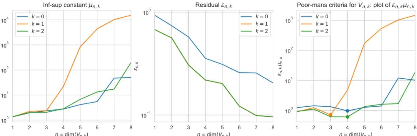
Figure 5.4). Yet, we can expect some bad artefacts in the reconstruction with this space since the true solution will be approximated by snapshots, some of which coming from the wrong part of the manifold and thus associated to the wrong partition of D. In addition, we can only work with nď m “ 8 and this may not be sufficient regarding the approximation power. Our estimator u˚0pwq uses the space Vn˚0,0, where the dimension n
˚
0 is the one that reaches
τ0 “ min1ďnďmµn,0εn,0as defined in (3.20) and (3.21). Figure 5.4 shows the product µn,0εn,0
for n“ 1, . . . , m and we see that n˚ 0 “ 3.
• Nonlinear method: We generate affine reduced bases spaces Vn,1 “ ¯u1 ` ¯Vn,1 and Vn,2 “
¯
u2 ` ¯Vn,2, each one specific for M1 and M2. Similarly as for the affine method, we take
as offsets ¯ui “ uipy “ 0q “ ¯u0, for i “ 1, 2, and we run two separate greedy algorithms
over ĂM1´ ¯u1 and ĂM2´ ¯u2 to build ¯Vn,1 and ¯Vn,2. We select the dimensions n˚k that reach
τk “ minn“1,...,mµn,kεn,k for k“ 1, 2. From Figure 5.4, we deduce 1
that n˚1 “ 4 and n˚2 “ 3.
This yields two estimators u˚
1pwq and u˚2pwq. We can expect better results than the affine
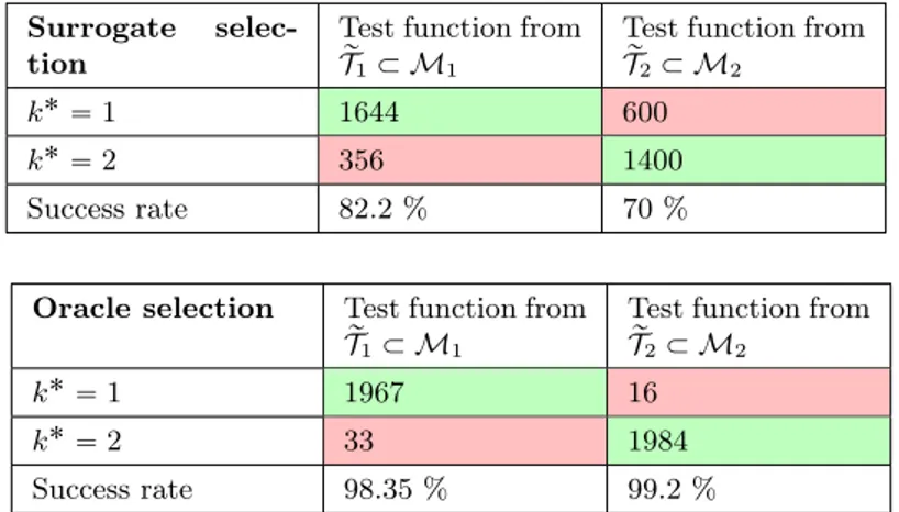
approach if we can detect well in which part of the manifold the target function is located. The main question is thus whether our model selection strategy outlined in Section 3.3 is able to detect well from the observed data w if the true u lies in M1 or M2. For this, we compute
the surrogate manifold distances
Spu˚kpwq, Mkq :“ min yPY Rkpu˚kpwq, yq, k“ 1, 2, (5.3) where Rkpu˚kpwq, yq :“ }divpakpyq∇u˚kpwqq ´ f }V1 1
Due to the spatial symmetry along the axis x` y “ 1 for the functions in ĂM1 and ĂM2, the greedy algorithm
selects exactly the same candidates to build Vn,2 as for Vn,1, except that each element is mirrored in the axis. One
may thus wonder why n˚ 1 ‰ n
˚
2. The fact that different values are chosen for each manifold reflects the fact that the
measurement space W introduces a symmetry break and the reconstruction scheme is no longer spatially symmetric contrary to the Vn,k.