ELECTRE TRI 2.0a : Methodological guide and user's documentation

ELECTRE TRI 2.0a

METHODOLOGICAL GUIDE

AND

USER'S MANUAL

V. Mousseau

, R. Slowinski

, P. Zielniewicz

1

LAMSADE, Universite Paris Dauphine, Place du Mare chal De Lattre de Tassigny, 75775 Paris cedex 16, France, tel: (+33-1) 44 05 41 84, Fax: (+33-1) 44 05 40 91, email: [email protected]. 2 _{Institute of Computing Science, Poznan University of Technology, Piotrowo 3a, 60-965 Poznan, Poland,}

1. GETTING STARTED 4

1.1 HARDWARE AND SOFTWARE REQUIREMENTS 4

1.2 SETTING UP THE SYSTEM 4

1.3 HOW TO GET INFORMATION 4

2. DESCRIPTION OF THE ELECTRE TRI METHOD 5

2.1 SOME BASIC CONCEPTS IN MULTIPLE CRITERIA DECISION AID 5

2.1.1 THE SORTING ”PROBLEMATIC„ OR PROBLEM STATEMENT 5

2.1.2 PREFERENCE MODELLING 6

2.1.3 OPERATIONAL APPROACHES TO DECISION AIDING 8

2.2 THE ELECTRE TRI METHOD 9

2.2.1 GENERAL PRESENTATION 9

2.2.2 THE OUTRANKING RELATION IN ELECTRE TRI 10

2.2.3 THE ASSIGNMENT PROCEDURES 18

2.2.4 CONSISTENCY IN THE DEFINITION OF THE CATEGORIES 21

3. ELECTRE-TRI ASSISTANT : ASSISTANCE IN THE CONSTRUCTION OF A PREFERENCE

MODEL SUPPORT FOR PARAMETER ELICITATION 22

3.1 INFERENCE OF PREFERENCE PARAMETERS 22

3.2 INTERACTIVE LEARNING PROCESS 22

4. SOFTWARE COMMANDS 25

4.1 USE OF THE SOFTWARE IN A DECISION AID PROCESS 25

4.2 GENERAL ORGANISATION 25

4.3 THE FILE MENU COMMANDS 26

4.3.1 NEW PROJECT 26

4.3.2 OPEN PROJECT 26

4.3.3 CLOSE PROJECT 26

4.3.4 SAVE PROJECT 27

4.3.5 SAVE PROJECT AS 27

4.3.6 IMPORT ALTERNATIVES FROM EXCEL 27

4.3.7 PROJECT REPORT 28

4.3.8 PRINT PROJECT 28

4.3.9 PRINT SETUP 28

4.3.10 EXIT 28

4.4 THE EDIT MENU COMMANDS 29

4.4.1 THE EDIT DATA SET COMMAND 29

4.4.2 ELECTRE TRI ASSISTANT 31

4.5.1 ASSIGNMENT BY CATEGORY 34 4.5.2 ASSIGNMENT BY ALTERNATIVE 34 4.5.3 COMPARISON TO PROFILES 34 4.5.4 PERFORMANCES OF ALTERNATIVES 34 4.5.5 DEGREES OF CREDIBILITY 34 4.5.6 VISUALISATION OF ALTERNATIVE 34 4.5.7 STATISTICS OF ASSIGNMENT 34

4.6 THE WINDOW MENU COMMANDS 35

4.6.1 CASCADE 35

4.6.2 TILE 35

4.6.3 ARRANGE ICONS 35

4.6.4 CLOSE ALL 35

4.7 HELP MENU COMMANDS 35

CONTENTS 35

4.7.2 SEARCH TOPIC 35

4.7.3 HOW TO USE HELP 35

4.7.4 ABOUT 35

5.A STEP-BY-STEP EXAMPLE 36

5.1 CREATING A NEW PROJECT 36

5.2 EDITING THE DATA SET 36

5.2.1 EDITING GENERAL INFORMATION 36

5.2.2 INSERTING AND EDITING CRITERIA 38

5.2.3 INSERTING AND EDITING PROFILES 42

5.2.4 INSERTING AND EDITING ALTERNATIVES 46

5.3 SAVING THE DATA SET 49

5.4 OBTAINING RESULTS 50

5.4.1 ASSIGNMENT BY CATEGORY 50

5.4.2 ASSIGNMENT BY ALTERNATIVE 50

5.4.3 INTERMEDIARY RESULTS 50

5.6 OPENING AN EXISTING PROJECT 54

5.7 LOADING DATA FROM THE PREVIOUS VERSION OF ELECTRE TRI 55

5.8 LOADING A SET OF ALTERNATIVES FROM EXCEL 56

5.9 AN ELECTRE TRI ASSISTANT SESSION 58

1. Getting started

1.1 Hardware and software requirements

The ELECTRE TRI Software version 2.0a is developed with the C++ programming language using the Microsoft Windows interface. The hardware and software requirements are the following:

• IBM-PC compatible computer with the following minimal RAM memory requirements: - Win 3.1: 8 Mb,

- Win 95: 16Mb.

• Microsoft Windows 3.1, 95 or higher.

1.2 Setting up the system

In order to install the ELECTRE TRI 2.0a software on your computer, please proceed as follows:

1. Create an Electre Tri 2.0 directory on your hard disk, 2. Insert the installation disk,

3. Copy the self-extracting file electre.exe in the directory you have created, 4. Run the exe self-extracting file from your hard disk.

1.3 How to get information

ELECTRE TRI is an existing multicriteria sorting method (see [Yu 92] and [Roy & Bouyssou 93]). The ELECTRE TRI 2.0 Software has been developed through a collaboration of two research teams :

• LAMSADE Laboratory3, University of Paris-Dauphine, France

• Institute of Computing Science4, Poznan University of Technology, Poznan, Poland To order the software, ask questions or make remarks, please contact :

Dominique Valle e

Lamsade - Universite Paris Dauphine Place du Mare chal De Lattre de Tassigny 75 775 Paris cedex 16 - France

tel: (33 1) 44 05 44 72 fax: (33 1) 44 05 40 91

email : [email protected]

3 _{LAMSADE - Universite Paris-Dauphine, Place du M}al

De Lattre de Tassigny, 75 775 Paris cedex 16, France.

2. Description of the ELECTRE TRI method

2.1 Some basic concepts in Multiple Criteria Decision Aid

2.1.1 The sorting ”problematicç or problem statement

In a given decision situation, it is possible to formulate the problem in different terms. Three different "problematics", i.e., problem formulations (choice, sorting and ranking) may guide the analyst in structuring the problem (see [Bana e Costa, 1996], [Bana e Costa, 1992]).

Among these problematics, a major distinction concerns relative versus absolute judgement of alternatives. This distinction refers to the way alternatives are considered and to the type of result expected from the analysis.

In the first case, alternatives are directly compared one to each other and the results are expressed using the comparative notions of better and worse. Choice (Selecting a subset A* of the best alternatives from A, see Figure 1) or ranking (definition of a preference order on A, see Figure 1) are typical examples of comparative judgements. The presence (or absence) of an alternative ak in the set of best alternatives A* results from the comparison of ak to the other

alternatives. Similarly, the position of an alternative in the preference order depends on its comparison to the others.

Titre: Auteur: Apercu:

Cette image EPS n'a pas e te enregistre e avec un apercu inte gre . Commentaires: Cette image EPS peut ˆ tre imprime e sur une imprimante PostScript mais pas sur un autre type d'imprimante.

Titre:

Auteur: Apercu:

Cette image EPS n'a pas e te enregistre e avec un apercu inte gre . Commentaires: Cette image EPS peut ˆ tre imprime e sur une imprimante PostScript mais pas sur un autre type d'imprimante.

Figure 1: Choice and ranking "problematics"

In the second case, each alternative is considered independently from the others in order to determine its intrinsic value by means of comparisons to norms or references; results are expressed using the absolute notions of "assign" or "not assign" to a category, "similar" or "not similar" to a reference profile, "adequate" or "not adequate" to some norms The sorting problematique (see Figure 2) refers to absolute judgement. It consists of assigning each alternative to one of the pre-existing categories which are defined by norms or typical elements of the category. The assignment of an alternative ak results from the intrinsic evaluation of ak on

criteria and from the norms defining the categories (the assignment of ak to a specific category

Titre: Auteur: Apercu:

Cette image EPS n'a pas e te enregistre e avec un apercu inte gre . Commentaires:

Cette image EPS peut ˆ tre imprime e sur une imprimante PostScript mais pas sur un autre type d'imprimante.

Figure 2: Sorting "problematic"

The semantic of the categories can imply an ordered structure on categories or not; the former case refers to ordered Multiple Criteria Sorting Problems (MCSP), the latter to nominal MCSP. MCSP differs from standard classification approach; the categories considered here are defined a priori and do not result from the analysis. These categories are usually conceived in such a way that alternatives assigned to the same category should be treated identically.

Previous works on MCSP have been developed using the outranking approach and several methods have been proposed: Trichotomic Segmentation (see [Moscarolla & Roy 77] and [Roy 81]), N-Tomic (see [Massaglia & Ostanello 91]), ORClass ([Larichev et al. 86] and [Larichev & Moshkovich 94]), ELECTRE TRI (see [Yu 92a], [Yu 92b] and [Roy & Bouyssou 93]). Filtering methods based on concordance and non-discordance principles have been studied in [Perny1aor98]. The use of rough sets theory ([Pawlak & Slowinski 94], [Slowinski 92] and [Greco et al. 98a]) has also allowed significant progress in this field.

Real world case studies of MCSP have been reported in the literature in various domains:

• evaluation of applicants for loans or grants ([Groleau et al. 95], [Veilleux et al. 96] and [Greco et al 98b]),

• business failure risk assessment ([Dimitras et al. 95], [Andenmatten 95]),

• screening methods prior to project selection ([Anandalingam & Olsson 89]),

• satellite shot planning ([Gabrel 94]),

• medical diagnosis ([Slowinski 92], [Tanaka et al. 92]),.

2.1.2 Preference modelling

Almost all decision aid studies involve the comparison of alternatives (either relative comparisons of couples of alternatives from A or comparisons of alternatives to norms represented by fictitious alternatives). The comparison of alternatives is naturally grounded on the consequences and attributes of these alternatives. We call criterion a real-valued function g that takes into account a specific viewpoint (grouping a class of homogenous consequences).

More precisely, a criterion g is a real-valued function mapping from A to ℜ, such that the comparison of any pair of alternatives a and b may be grounded on the comparison of the two values g(a) and g(b).

The direction of preference on a criterion can be increasing or decreasing. In the first case, the higher the evaluation g(a), the better is a with respect to the criterion g (quality criterion); in the second case, a criterion with a decreasing direction of preference corresponds to a criterion g on which the performance of an alternative a decreases when g(a) increases (cost criterion). Without any loss of generality, we will suppose in this section that the direction of preference is increasing for all criteria.

Ideally, so as to enable the comparison of any pair of alternatives a and b in A, a criterion g should be constructed such that :

    ⇒ > ⇒ = b g aP b g a g b g aI b g a g ) ( ) ( ) ( ) ( [1]

where Ig and Pg denote the indifference and strict preference relations relatively to criterion g.

In practical situations, the evaluation of alternatives are very often subject to imprecision, uncertainty and ill determination. Consequently, a small difference of evaluation g(a)-g(b) can also imply an indifference situation. Moreover, even when this difference does not seems negligeable, it does not always reflect a preference situation.

It is then more reasonable and prudent to consider a more general model of criterion (the preceding one being a specific case) in which the function g should be constructed so that:g(a)≥g(b)⇒aS_gb where aSgb means ”a is at least as good as bç (or a outranks b)

according to criterion g.

In order to account for the imprecision, uncertainty and ill determination of the data, it is common to use discrimination thresholds that identify the limits between situations of indifference and strict preference. Two values q and p are introduced such that :

      ⇒ > − ⇒ ≤ − < ⇒ ≤ − b g aP p b g a g b g aQ p b g a g q b g aI q b g a g ) ( ) ( ) ( ) ( ) ( ) ( [2]

where Qg denotes the weak preference relation relatively to criterion g. A weak preference

relation is an intermediate situation that account for a hesitation between the situations of indifference and strict preference.

q and p are called indifference and preference threshold, respectively. In the general case, these thresholds may vary with the evaluations (see Figure 3).

The model of true-criterion defined in [1] corresponds to the case where p=q=0. The general model (q≥0 and p≥0) is called pseudo-criterion ; two interesting specific cases are the semi-criterion when q=p and the pre-criterion when q=0.

Assigning a value to these thresholds is a difficult practical problem. Such values can be either determined after analysing the imprecision of the data or inferred using the ELECTRE TRI Assistant functionalities (see section 3). However, it is important to stress that, in a constructivist approach, it seems illusory to try to approximate ”true valueç for these parameters. These ”reasonable valuesç whose impact are to be studied through a

robustness analysis. It consists in exploring the impact of the variations of the parameters on the strength of the resulting conclusions.

Titre: Auteur: Apercu:

Cette image EPS n'a pas e te enregistre e avec un apercu inte gre . Commentaires:

Cette image EPS peut ˆ tre imprime e sur une imprimante PostScript mais pas sur un autre type d'imprimante.

Figure 3: Pseudo-criterion

2.1.3 Operational approaches to decision aiding

In multicriteria analysis, there are three ways to proceed when facing a problem for which a prescription or recommendation is to be derived through the aggregation of performances of alternatives.

2.1.3.1 Use of a single synthesising criterion

When the criteria are rather homogenous, and total compensation between criteria is acceptable, it is frequent to build a single criterion function that accounts for all pertinent aspects of the problem. In this case, the evaluations of an alternative may be synthesised in a single value. Alternatives are then mutually comparable, as the comparisons is made by the mean of comparison s of numbers. Moreover, this way to proceed induce a transitive preference relation. Let us remark that classical methods such as the weighted sum typically refers to this approach.

2.1.3.2 Synthesising by outranking with incomparabilities

This approach relies on an aggregation rule that allows situations of incomparability, refusing a priori a total compensation between criteria. Incomparability is accepted so as to avoid arbitrary or fragile judgements. Moreover, transitivity of the outranking relation is not systematically imposed. Let us note that all ELECTRE type methods refer to this approach.

2.1.3.3 Interactive local judgements with trial-and-error iterations

This approach consist in highlighting a prescription for the decision problem through a sequence of question-answer. Each interactive procedure is grounded on an interaction protocol composed of dialogue and computing phases. The interaction stops when the decision maker is satisfied with the last proposal of the procedure.

2.2 The ELECTRE TRI method

2.2.1 General presentation

ELECTRE TRI assigns alternatives to predefined categories. The assignment of an alternative a results from the comparison of a with the profiles defining the limits of the categories. Let F denote the set of the indices of the criteria g1, g2, ..., gm (F={1, 2, ..., m}) and B

the set of indices of the profiles defining p+1 categories (B={1,2,...,p}), bh being the upper limit

of category Ch and the lower limit of category Ch+1, h=1, 2, ...,p (see Figure 4). In what follows,

we will assume, without any loss of generality, that preferences increase with the value on each criterion.

Schematically, Electre Tri assigns alternatives to categories following two consecutive steps :

• construction of an outranking relation S that characterises how alternatives compare to the limits of categories,

• exploitation (through assignment procedures) of the relation S in order to assign each alternative to a specific category.

Figure 4: Ordered categories defined by limit profiles

ELECTRE TRI builds an outranking relation S, i.e., validates or invalidates the assertion aSbh (and bhSa), whose meaning is "a is at least as good as bh". Preferences restricted to the

significance axis of each criterion are defined through pseudo-criteria (see [Roy & Vincke 84] for details on this double-threshold preference representation). The indifference and preference thresholds (qj(bh) and pj(bh)) constitute the intra-criterion preferential information. They account

for the imprecise nature of the evaluations gj(a) (see [Roy 89]). qj(bh) specifies the largest

difference gj(a)-gj(bh) that preserves indifference between a and bh on criterion gj; pj(bh)

represents the smallest difference gj(a)-gj(bh) compatible with a preference in favor of a on

criterion gj.

At the comprehensive level of preferences, in order to validate the assertion aSbh (or

• concordance: for an outranking aSbh (or bhSa) to be accepted, a "sufficient" majority

of criteria should be in favour of this assertion,

• non-discordance: when the concordance condition holds, none of the criteria in the minority should oppose to the assertion aSbh (or bhSa) in a "too strong way".

Two types of inter-criteria preference parameters intervene in the construction of S:

• the set of weight-importance coefficients (k1,k2, ..., km) is used in the concordance test

when computing the relative importance of the coalitions of criteria being in favour of the assertion aSbh,

• the set of veto thresholds (v1(bh),v2(bh), ..., vm(bh)), ∀h∈B, is used in the discordance

test. vj(bh) represents the smallest difference gj(bh)-gj(a) incompatible with the

assertion aSbh.

2.2.2 The outranking relation in ELECTRE TRI

In the ELECTRE TRI method, an outranking relation is build in order to enable the comparison of an alternative a to a profile bh. This outranking relation is build through the

following steps:

• compute the partial concordance indices cj(a,bh) and cj(bh,a), • compute the overall concordance indices c(a,bh),

• compute the partial discordance indices dj(a,bh) and dj(bh,a),

• compute the fuzzy outranking relation grounded on the credibility indices σ(a,bh), • determine a λ-cut of the fuzzy relation in order to obtain a crisp outranking relation.

2.2.2.1 Partial concordance indices

The partial concordance index cj(a,bh) (cj(bh,a), respectively) expresses to which extend

the statement ”a is at least as good as bh (bh is at least as good as a, respectively) considering

criterion gjç. When gj has an increasing direction of preference, index cj(a,bh) and cj(bh,a) are

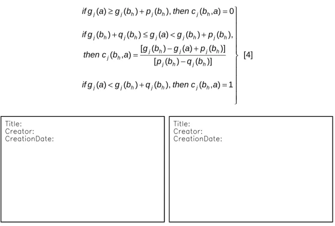
computed as follows (see Figure 5):

             = < − − + − = − ≤ < − = − ≤ 1 ) , ( ), ( ) ( ) ( )] ( ) ( [ )] ( ) ( ) ( [ ) , ( ), ( ) ( ) ( ) ( ) ( 0 ) , ( ), ( ) ( ) ( h j j h j h j h j h j h j h j j h j h j h j j h j h j h j h j h j j b a c then a g b q b g if b q b p b p b g a g b a c then b q b g a g b p b g if b a c then b p b g a g if [3]

             = + < − + − = + < ≤ + = + ≥ 1 ) , ( ), ( ) ( ) ( )] ( ) ( [ )] ( ) ( ) ( [ ) , ( ), ( ) ( ) ( ) ( ) ( 0 ) , ( ), ( ) ( ) ( a b c then b q b g a g if b q b p b p a g b g a b c then b p b g a g b q b g if a b c then b p b g a g if h j h j h j j h j h j h j j h j h j h j h j j h j h j h j h j h j j [4]

Figure 5: cj(bh,a) and cj(a,bh), increasing direction of preference

When gj has a decreasing direction of preference, index cj(a,bh) and cj(bh,a) are computed as

follows (see Figure 6):

             = > + − + − = + ≤ ≤ + = + ≥ 1 ) , ( ), ( ) ( ) ( )] ( ) ( [ )] ( ) ( ) ( [ ) , ( ), ( ) ( ) ( ) ( ) ( 0 ) , ( ), ( ) ( ) ( h j j h j h j h j h j h j j h j h j h j h j j h j h j h j h j h j j b a c then a g b q b g if b q b p b p a g b g b a c then b p b g a g b q b g if b a c then b p b g a g if [5]              = − > − + − = − < ≤ − = − ≤ 1 ) , ( ), ( ) ( ) ( )] ( ) ( [ )] ( ) ( ) ( [ ) , ( ), ( ) ( ) ( ) ( ) ( 0 ) , ( ), ( ) ( ) ( a b c then b q b g a g if b q b p b p b g a g a b c then b q b g a g b p b g if a b c then b p b g a g if h j h j h j j h j h j h j h j j h j h j h j j h j h j h j h j h j j [6]

Figure 6: cj(bh,a) and cj(a,bh), decreasing direction of preference

2.2.2.2 Global concordance indices

Global concordance indices c(bh,a) (c(a,bh), respectively) express to which extend the

evaluations of a and bh on all criteria are concordant with the assertion ”a outranks bhç (”bh

outranks aç, respectively). c(bh,a) and c(a,bh) are computed as follows:

∑

∑

∑

∑

The partial discordance index dj(a,bh) (dj(bh,a), respectively) expresses to which extend

the criterion gj is opposed to the assertion ”a is at least as good as bhç, i.e., ”a outranks bh (”bh

is at least as good as aç, respectively). A criterion gj is said to be discordant with to assertion ”a

outranks bh is on this criterion bh is preferred to a (bh P a, i.e., cj(bh,a)=1 and cj(a,bh)=0). In the

case of increasing preferences, the criterion gj opposes a veto when the difference gj(bh)-gj(a)

exceeds the veto threshold vj(bh).

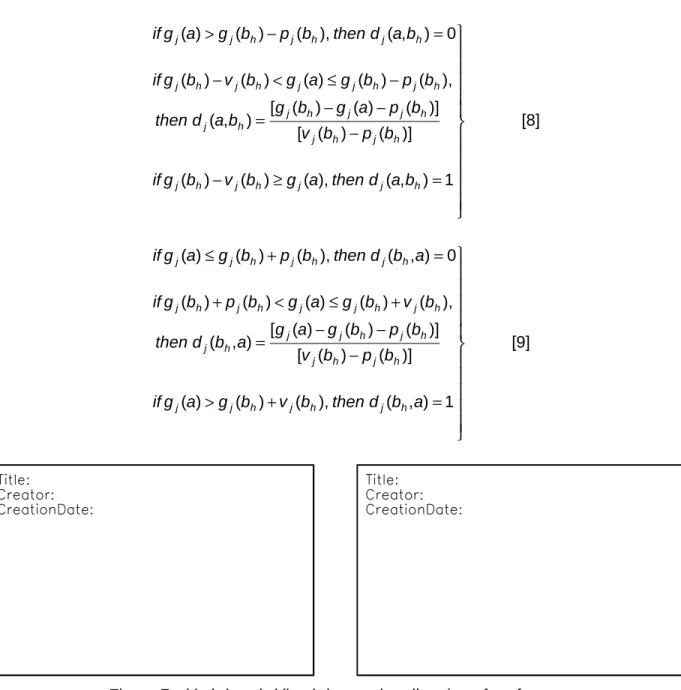
When gj has an increasing direction of preference, dj(a,bh) and dj(bh,a) are computed as

             = ≥ − − − − = − ≤ < − = − > 1 ) , ( ), ( ) ( ) ( )] ( ) ( [ )] ( ) ( ) ( [ ) , ( ), ( ) ( ) ( ) ( ) ( 0 ) , ( ), ( ) ( ) ( h j j h j h j h j h j h j j h j h j h j h j j h j h j h j h j h j j b a d then a g b v b g if b p b v b p a g b g b a d then b p b g a g b v b g if b a d then b p b g a g if [8]              = + > − − − = + ≤ < + = + ≤ 1 ) , ( ), ( ) ( ) ( )] ( ) ( [ )] ( ) ( ) ( [ ) , ( ), ( ) ( ) ( ) ( ) ( 0 ) , ( ), ( ) ( ) ( a b d then b v b g a g if b p b v b p b g a g a b d then b v b g a g b p b g if a b d then b p b g a g if h j h j h j j h j h j h j h j j h j h j h j j h j h j h j h j h j j [9]

Figure 7: dj(a,bh) and dj(bh,a), increasing direction of preference

When gj has a decreasing direction of preference, dj(a,bh) and dj(bh,a) are computed as

follows (see Figure 8):

            = < + − − − = + ≤ < + = + ≤ 1 ) , ( ), ( ) ( ) ( )] ( ) ( [ )] ( ) ( ) ( [ ) , ( ), ( ) ( ) ( ) ( ) ( 0 ) , ( ), ( ) ( ) ( h j j h j h j h j h j h j h j j h j h j h j j h j h j h j h j h j j b a d then a g b v b g if b p b v b p b g a g b a d then b v b g a g b p b g if b a d then b p b g a g if [10]

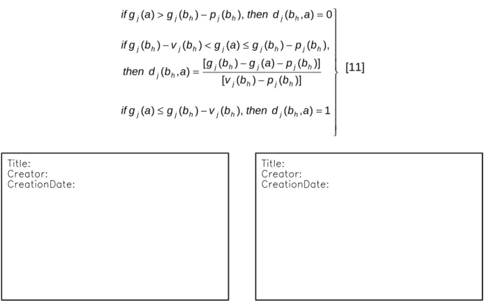
             = − ≤ − − − = − ≤ < − = − > 1 ) , ( ), ( ) ( ) ( )] ( ) ( [ )] ( ) ( ) ( [ ) , ( ), ( ) ( ) ( ) ( ) ( 0 ) , ( ), ( ) ( ) ( a b d then b v b g a g if b p b v b p a g b g a b d then b p b g a g b v b g if a b d then b p b g a g if h j h j h j j h j h j h j j h j h j h j h j j h j h j h j h j h j j [11]

Figure 8: dj(a,bh) and dj(bh,a), decreasing direction of preference

2.2.2.4 Degree of credibility of the outranking relation

The degree of credibility of the outranking relation σ(a,bh) (σ(bh,a), respectively)

expresses to which extend ”a outranks bhç (”bh outranks aç, respectively) according to the global

concordance index c(a,bh) and to the discordance indices dj(a,bh), ∀j∈F (according to the global

concordance index c(bh,a) and to the discordance indices dj(bh,a)), ∀j∈F, respectively).

Computing the credibility indices σ(a,bh) and σ(bh,a) amounts at establishing a valued

outranking relation.

The computation of the credibility index σ(a,bh) is grounded on the following principles:

1) when no criteria are discordant, the credibility of the outranking relation σ(a,bh) is

equal to the concordance index σ(a,bh),

2) when a discordant criterion opposes a veto to the assertion ”a outranks bhç (i.e.,

dj(a,bh)=1), then credibility index σ(a,bh) becomes null (the assertion ”a outranks bhç

is not credible at all),

3) when a discordant criterion is such that c(a,bh)<dj(a,bh)<1, the credibility index σ(a,bh)

becomes lower than the concordance index c(a,bh), due to the effect of the

opposition on this criterion.

It results from these principles that the credibility index σ(a,bh) corresponds to the concordance

index c(a,bh) weakened by eventual veto effects. More precisely, the value of σ(a,bh) is

∏

{

}

2.2.2.5 Resulting outranking relation

The translation of the obtained fuzzy outranking relation into a crisp outranking relation S is done by means of a λ-cut, (λ is called cutting level). λ is considered as the smallest value of the credibility index compatible with the assertion ”a outranks bhç, i.e., σ(a,bh)≥λ ⇒ aSbh.

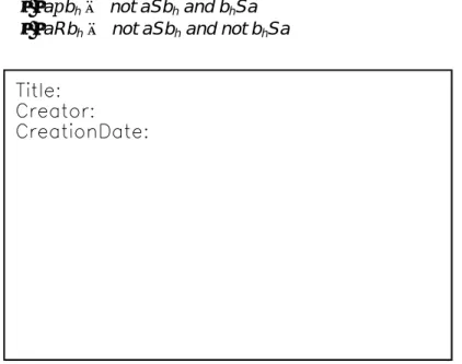
We define the binary relations f (preference), I (indifference) and R (incomparability) as follow (see Figure 9):

• aIbh⇔ aSbh and bhSa • afbh⇔ aSbh and not bhSa • apbh⇔ not aSbh and bhSa • aRbh⇔ not aSbh and not bhSa

Figure 9: Definition of the binary relations f, I and R

2.2.2.6 A numerical example

Let us consider three alternatives a1, a2 and a3 evaluated on five criteria g1, g2, g3, g4 and

g5. Let us suppose that the direction of preference on each criterion is increasing and that

maximum and minimum evaluation on all criteria is 100 and 0, respectively. The evaluation matrix is given in Table 1.

g1 g2 g3 g4 g5

a1 75 67 85 82 90

a2 28 35 70 90 95

a3 45 60 55 68 60

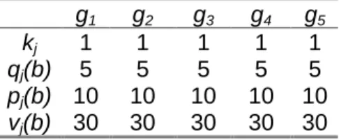
Let us suppose that the alternatives are to be compared to the profile b=(70, 75, 80, 75, 85) using the preferential information given in Table 2:

g1 g2 g3 g4 g5

kj 1 1 1 1 1

qj(b) 5 5 5 5 5

pj(b) 10 10 10 10 10

vj(b) 30 30 30 30 30

Table 2: Preference parameters

Comparison of a1 and b:

1) computation of partial concordance indices cj(b,a1) and cj(a1,b), (see è 2.2.2.1)

g1 g2 g3 g4 g5

cj(a1,b) 1 0.4 1 1 1

cj(b,a1) 1 1 1 1 1

Table 3: Partial concordance indices cj(b,a1) and cj(a1,b)

2) computation of the concordance indices c(b,a1) and c(a1,b),

[

]

[

]

3) computation of the discordance indices dj(a1,b) and dj(b,a1),

g1 g2 g3 g4 g5

dj(a1,b) 0 0 0 0 0

dj(b,a1) 0 0 0 0 0

Table 4: Discordance indices dj(b,a1) and dj(a1,b)

4) computation of the credibility indices σ(a1,b) andσ(b,a1),

σ σ ( , ) ( , ) . ( , ) ( , ) a b c a b b a c b a 1 1 1 1 0 88 1 = = = = as dj(a b1, )=dj( ,b a1)= ∀ ∈0, j F

5) determination of the preference relation between a1 and b (λ=0.75)

σ λ σ λ ( , ) ( , ) a b a Sb b a bSa a Ib 1 1 1 1 1 ≥ ⇒ ≥ ⇒    ⇒

Comparison of a2 and b:

1) computation of the partial concordance indices cj(b,a2) and cj(a2,b), (see è 2.2.2.1)

g1 g2 g3 g4 g5

cj(a2,b) 0 0 0 1 1

cj(b,a2) 1 1 1 0 0

Table 5: Partial concordance indices cj(b,a2) and cj(a2,b)

2) computation of the concordance indices c(b,a2) and c(a2,b),

[

]

[

]

3) computation of the discordance indices dj(a2,b) and dj(b,a2),

g1 g2 g3 g4 g5

dj(a2,b) 1 1 0 0 0

dj(b,a2) 0 0 0 0.25 0

Table 6: Discordance indices dj(b,a2) and dj(a2,b)

4) computation of the credibility indices σ(a2,b) andσ(b,a2),

σ( , )a₂ b =0 as d_j(a₂, )b =1, for j =12,

σ( , )b a₂ =0 6. as d_j( ,b a₂)<c a( ₂, ),b ∀ ∈j F

5) determination of the preference relation between a2 and bh (λ=0.75)

σ λ σ λ ( , ) ( , ) a b not a Sb b a not bSa a Rb 2 2 2 2 2 < ⇒ < ⇒    ⇒ Comparison of a3 and b:

1) computation of the partial concordance indices cj(b,a3) and cj(a3,b), (see è 2.2.2.1)

g1 g2 g3 g4 g5

cj(a3,b) 0 0 0 0.6 1

cj(b,a3) 1 1 1 1 1

2) computation of the concordance indices c(b,a3) and c(a3,b),

[

]

[

]

3) computation of the discordance indices dj(a3,b) and dj(b,a3),

g1 g2 g3 g4 g5

dj(a3,b) 0.75 0.25 0.75 0 0.75

dj(b,a3) 0 0 0 0 0

Table 8: Discordance indices dj(b,a3) and dj(a3,b)

4) computation of the credibility indices σ(a3,b) andσ(b,a3),

σ( , ) . . . . . . . . . a₃ b 0 12 1 0 75 1 0 12 1 0 25 1 0 12 1 0 75 1 0 12 1 0 75 1 0 12 0 = × −₋ × −₋ × −₋ × −₋ ≈ σ( , )b a₃ =c b a( , ₃)=1as d_j( ,b a₃)= ∀ ∈0, j F

5) determination of the preference relation between a3 and bh (λ=0.75)

σ λ σ λ ( , ) ( , ) a b not a Sb b a bSa a b 3 3 3 3 3 < ⇒ ≥ ⇒    ⇒ p

2.2.3 The assignment procedures

The role of the exploitation procedure is then to analyse the way in which an alternative a compares to the profiles so as to determine the category to which a should be assigned. Two assignment procedures are available.

2.2.3.1 the pessimistic assignment procedure

Pessimistic (or conjunctive) procedure :

a) compare a successively to bi, for i=p,p-1, ..., 0,

b) bh being the first profile such that aSbh, assign a to category Ch+1 (a → Ch+1).

If bh-1 and bh denote the lower and upper profile of the category Ch, the pessimistic

procedure assigns alternative a to the highest category Ch such that a outranks bh-1, i.e., aSbh-1.

When using this procedure with λ=1, an alternative a can be assigned to category Ch only if

gj(a) equals or exceeds gj(bh-1) (by some threshold) for each criterion (conjunctive rule). When λ

decreases, the conjunctive characters of this rule is weakened.

2.2.3.2 the optimistic assignment procedure

Optimistic (or disjunctive) procedure :

b) bh being the first profile such that bh f a, assign a to category Ch (a → Ch).

The optimistic (or disjunctive) procedure assigns a to the lowest category Ch for which

the upper profile bh is preferred to a, i.e., bhfa. When using this procedure with λ=1, an

alternative a can be assigned to category Ch when gj(bh) exceeds gj(a) (by some threshold) at

least for one criterion (disjunctive rule). When λ decreases, the disjunctive character of this rule is weakened.

2.2.3.3 Comparison of the two assignment procedures

The ideas that ground the two assignment procedures are different; consequently, it is not surprising that these assignment procedures might assign some alternatives to different categories. The following result explains, on a theoretical level the reason of potential divergence of the assignment results.

Let us suppose that an alternative a is assigned to Ci and Cj by the pessimistic and

optimistic assignment rule respectively. It holds :

• Ci is lower or equal to Cj (i≤j),

• Ci is greater than Cj when a is incomparable with all profiles between Ci and Cj (aRbf,

∀f such that j≤f<i). More specifically :

• when the evaluation of an alternative are between the two profiles of a category on each criterion, then both procedure assign this alternative to this category,

• a divergence exists among the results of the two assignment procedures only when an alternative is incomparable to one or several profiles; in such case the pessimistic assignment rule assigns the alternative to a lower category than the optimistic one.

2.2.3.4 Illustrative example

Let us consider the example presented in è 2.2.2.6 in which we face a trichotomic segmentation problem. The three categories C1, C2 and C3 are delimited by two profiles b1 and

b2. b1 represents the ”frontierç between C1 and C2 (b1 is the lower limit of C2 and the upper limit

of C1) b2 represents the ”frontierç between C2 and C3 (b2 is the lower limit of C3 and the upper

limit of C2). These two profiles are defined in Table 9. b0 and b3 are two extreme profiles

representing the anti-ideal and ideal alternatives (it holds afb0 and b3pa, ∀a).

g1 g2 g3 g4 g5

b1 50 48 55 55 60

b2 70 75 80 75 85

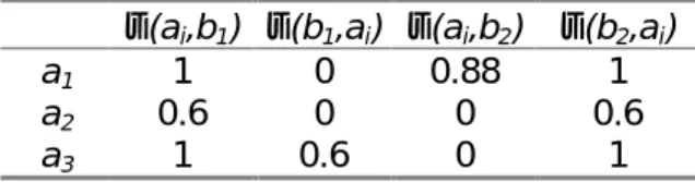
The credibility indices of the outranking relation between the alternatives to be assigned (a1, a2 and a3) and the profiles (b1 and b2) is computed as defined in è 2.2.2. The results are

presented in Table 10.

σ(ai,b1) σ(b1,ai) σ(ai,b2) σ(b2,ai)

a1 1 0 0.88 1

a2 0.6 0 0 0.6

a3 1 0.6 0 1

Table 10: Credibility indices σ(ai,bh)

If we set λ=0.75, the resulting preference relations between ai and bh are the following (see

Table 11):

b1 b2

a1 f I

a2 R R

a3 f p

Table 11: Preference relations between ai and bh

Results of ELECTRE TRI pessimistic assignment procedure:

a1 is assigned to C3 because a1Sb3 does not hold but a1Sb2 holds.

a2 is assigned to C1 because a2Sb3, a2Sb2 and a2Sb1 do not hold but a2Sb0 holds.

a3 is assigned to C2 because a3Sb3 and a3Sb2 do not hold but a3Sb1 holds.

Results with ELECTRE TRI optimistic assignment procedure:

a1 is assigned to C3 because b0fa1, b1fa1 and b2fa1 do not hold but b3fa1,holds.

a2 is assigned to C3 because b0fa2, b1fa2 and b2fa2 do not hold but b3fa2,holds.

a3 is assigned to C2 because b0fa3 and b1fa3 do not hold but b2fa3,holds.

Let us remark that a2 is assigned to C3 by the optimistic assignment procedure, and to C1

by the pessimistic assignment procedure. This difference among the two results stems from the fact that a2 is incomparable to both profiles b1 and b2.

2.2.4 Consistency in the definition of the categories

The ordered p+1 categories C1, C2, ..., Cp+1 are defined in ELECTRE TRI by p profiles b1, b2, ...,

bp, bh being the upper limit of category Ch and the lower limit of category Ch+1, h=1, 2, ...,p. For

the categories to be consistently defined, the profiles should respect the two following conditions:

Condition 1 : ∀j∈F, ∀h=1..p-1, gj(bh+1) ≥ gj(bh)

This condition simply states that the categories should be ordered. As ELECTRE TRI considers ordered categories, it is not possible to use the method if this condition is not fulfilled.

Condition 2 : ∀j∈F, ∀h=1..p-1, gj(bh+1) - pj(bh+1) ≥ gj(bh) + pj(bh)

In order to define ”distinguishableç categories, it is reasonable to impose that no alternative can be indifferent to more than one profile, i.e., ∀a∈A, ∀h=1..p-1, aIbh⇒ [not aIbh+1 and not aIbh-1]

(a situation in which aIbh and aIbh+1 would implicitly mean that the category delimited by the

profiles bh and bh+1 is ”insufficiently wideç). Condition 2 is a sufficient condition for the

preceeding property to hold. In other words, it is possible to run ELECTRE TRI with profiles that do not fulfill condition 2 but in such cases some alternatives can be indifferent to two consecutive profiles.

3. ELECTRE-TRI Assistant : Assistance in the construction of

a preference model Support for Parameter Elicitation

3.1 Inference of preference parameters

One of the main difficulties that an analyst must face when interacting with a DM in order to build a decision aid procedure is the elicitation of various parameters of the DM's preference model. In the ELECTRE TRI method, the analyst should assign values to profiles, weights and thresholds (see section 2). Even if these parameters can be interpreted, it can be difficult to fix directly their values and to have a clear global understanding of the implications of these values in terms of the output of the model.

[Mousseau & Slowinski 98] proposed a methodology that encompasses this problem by substituting assignment examples for direct elicitation of the model parameters. The values of the parameters are inferred through a certain form of regression on assignment examples. ELECTRE TRI Assistant implements this methodology in a way that requires from the DM much less cognitive effort: the elicitation of parameters is done indirectly (rather than directly) using holistic information given by the DM through assignment examples, i.e., alternatives assigned by the DM according to his/her preferences.

Assuming that a specific subset of parameters (possibly all of them) is to be optimised, mathematical program infers the values for these parameters that best restitutes the assignment examples (the general form of the mathematical program to be solved is given in appendix A). This is done in the course of an interactive process that gives to the DM the possibility to revise his/her assignment examples and/or change the set of parameters to be determined and/or to give additional information before the optimisation phase restarts.

The general scheme of this inference procedure using the paradigm of disaggregation is presented in Figure 10. Its aim is to find an ELECTRE TRI model as compatible as possible with the assignment examples given by the DM. The assignment examples concern a subset A*⊆A of alternatives for which the DM has clear preferences, i.e., alternatives that the DM can easily assign to a category, taking into account their evaluation on all criteria. The compatibility between the ELECTRE TRI model and the assignment examples is understood as an ability of the ELECTRE TRI method using this model to reassign the alternatives from A* in the same way as the DM did.

3.2 Interactive learning process

In order to minimise the differences between the assignments made by ELECTRE TRI and the assignments made by the DM, an optimisation procedure is used. The resulting ELECTRE TRI model is denoted by M_π. The DM can tune up the model in the course of an interactive procedure (see Figure 10). He/she may either (1) revise the assignment examples or (2) change the set of parameters to be optimised or (3) fix values (or intervals of variation) for some model parameters. In the first case, the DM may:

• remove and/or add some alternatives from/to A*,

In the second case, he/she may remove and/or add some parameters from the set of those that are to be optimised.

In the last case, the DM can give additional information on the range of variation of some model parameters basing on his/her own intuition. For example, he/she may specify:

• ordinal information on the importance of criteria,

• noticeable differences on the scales of criteria,

• incomplete definition of some profiles defining the limits between categories.

Figure 10: Inference scheme with ELECTRE TRI Assistant

When the model is not perfectly compatible with the assignment examples, the procedure is able to detect all "hard cases", i.e., the alternatives for which the assignment computed by the model strongly differs from the DM's assignment. The DM is then asked to reconsider his/her judgement.

To get a representative model, the subset A* must be defined such that the numbers of alternatives assigned to the categories are almost equal and sufficiently large to "contain enough information". The empirical behaviour of the inference procedure has been studied in [Naux 96] and [Mousseau et al. 97]. These experiments show that 2m (m being the number of criteria) is a sufficient number of assignment examples to infer the weights (the other parameters being fixed). Moreover, these studies proves the inference procedure to be suited for the interactive process described above.

The approach used in ELECTRE TRI Assistant is concordant with aggregation-disaggregation paradigm used for the construction of a preference model in UTA-like procedures (see [Jacquet-Lagr`ze & Siskos 82], [Siskos & Yanacopoulos 85], [Yanacopoulos 85], [Jacquet-Lagr`ze et al. 87], [Jacquet-Lagr`ze 90], [Nadeau et al. 90], [Slowinski 91]). It has been also applied for the elicitation of weights used for the construction of an outranking relation in the DIVAPIME method (see [Mousseau 95] and [Mousseau 93]).

In order to infer the parameters of Electre Tri pessimistic assignment procedure (without veto) from assignment examples, optimization problem to be solved is the following:

(

)

(

)

[

]

∑

∑

∑

∑

∑

where xk and yk represents slack variables whose meaning is such that all alternatives from the

reference set A* are "correctly" assigned for all '

[

]

k

k∈ + ∈

−

∈ λ λ

λ . When

ε=0, any non-negative value for the objective function guarantees existence of model parameters that permits "correct" assignment of all alternatives from A*.

The above general problem is a non-linear programming problem. For n, m and p denoting the number of assignment examples, of criteria and of profiles, respectively, this problem contains 3mp+m+2 variables and 4n+3mp+2 constraints.

The optimization problem becomes linear when optimization is limited to the inference of weights.

When additional preference information on dependencies among the weights or on the range of their variation is given, additional constraints should be considered in the above formulation.

4. Software commands

4.1 Use of the software in a decision aid process

Real world decision processes are never sequential; the different phases in the definition of an assignment model interact (for example, the assignment of some alternative may reveal the necessity to consider an additional criterion). However, the general scheme of a decision aid process using the ELECTRE TRI method can be presented as shown in Figure 11.

Figure 11: General scheme of use of the ELECTRE TRI method

4.2 General organisation

The structure of the main menu available in the ELECTRE TRI 2.0a software is described in Figure 12. The content of the different options are the following:

• File: this option allows the user to create a new project, load an existing project and

save the current project. Additional print and import options are provided.

• Edit: enables the user to enter the data required by ELECTRE TRI (criteria,

alternatives, weights, profiles and thresholds) and/or to use the ELECTRE TRI assistant commands.

• Results: allows the user to visualise the results (including intermediary results such

as degree of credibility of the outranking relation, comparison of alternatives to profiles,...); also gives a graphical representation of alternatives and profiles.

• Windows: gives the possibility to manage the appearance of the windows on the

screen.

Titre:

Auteur:

Apercu:

Cette image EPS n'a pas e te enregistre e avec un apercu inte gre . Commentaires:

Cette image EPS peut ˆ tre imprime e sur une imprimante PostScript mais pas sur un autre type d'imprimante.

Figure 12: Structure of the software options

4.3 The File menu commands

4.3.1 New project

This command allows to create a new project. This new project will be associated to a new data set that you will have to create. This command leads you to the Edit Project Dialog box in which the data concerning the project can be entered.

The first button in the Tool bar is a short-cut for this command.

4.3.2 Open project

This command may be used to load in memory a data set created during a previous session of ELECTRE and that has been saved on disk.

The second button in the Tool bar is a short-cut for this command.

You have to type the name of the project or to select it in the file list. You may choose the drive on which your file is saved and the directory in the Directories list box window. The

Files of type combo box gives a list of all files that have the mask proposed in the File Name

list box window. By default, ELECTRE gives a list of the files having the extension .BDF and .ELP in the current directory.

It is also possible to import data from the previous version of ELECTRE TRI using the Files

of type combo box, and selecting <Electre Tri 1.0 files>.

4.3.3 Close project

This command may be used to remove from memory the current data set. If you want to keep your dataset, you must use the Save project command before using this command.

However, if the current project was changed, the Save project as dialog box will be displayed automatically.

4.3.4 Save project

This command allows to save the project currently in memory with its current name. It can only be used when a project has previously been created or loaded.

The third button in the Tool bar is a short-cut for this command.

If the project has just been created, ELECTRE TRI displays the dialog box Save Project As so that you may give a name to your project.

4.3.5 Save project As

This command allows to save the current project under a name different from its current name or to save a project for the first time.

To save a project with its current name, you should use the Save project command. Choose the drive and the directory in the Directories list box window and type the name of the file in the File Name list box window. If you do not give any extension to the file name, ELECTRE TRI will add the extension .BDF. If you type an existing file name in the chosen directory, ELECTRE TRI will ask confirmation before removing the existing file.

4.3.6 Import alternatives from a text file

This command may be used to import the data (only the alternatives) from the an ASCII file in a specific format (see also è 5.8 for more information). The text file contain on each of its lines the information concerning a single alternative with the following format:

• the name of the alternative (string up to 8 characters without any spaces) in the first column,

• column separator (<TAB> character),

• the description of the alternative (string up to 255 characters without any spaces) in the second column,

• column separator (<TAB> character),

• the performances of the alternative (numeric values between -999999 and +999999 with a dot (.) as decimal separator) in the next columns. Each performance should be separated by the <TAB> character.

4.3.7 Project Report

This command may be used to generate a report (.RPT ascii file) on the current project. This file contains the following information :

• list of criteria,

• list of profiles and corresponding thresholds,

• list of all alternatives.

4.3.8 Print project

This command allows to print all or part of the data and/or the results. You have to select the elements you wish to print.

The fourth button in the Tool bar is a short-cut for this command.

Use the Print Setup command to choose the printer and to define printing parameters. You may also print in a file (see Print setup).

4.3.9 Print setup

This command may be used to choose the printer and to define printing parameters such as the orientation (Portrait or Landscape). These parameters depend on the selected printer. The printers that are displayed are those installed with Windows. To add new printers, you have to use the Control Panel of Windows.

4.3.10 Exit

This command closes ELECTRE TRI. You also may double-click on the System box of the window ELECTRE TRI or type ALT-F4.

If the current project has been modified since it has last been saved on disk, ELECTRE TRI will ask if you would like to save before exiting.

4.4 The Edit menu commands

4.4.1 The Edit Data set command

This command may be used to visualise and/or modify all data related to the project, i.e., information concerning the owner and description of the project, the criteria, the profiles defining the categories, the alternatives.

The fifth button in the Tool bar (displaying a folder) is a short-cut for this command.

The button enables the user to insert a criterion, a profile or an alternative (according to the element selected on the left part of the dialog window).

The button enables the user to delete the criterion, the profile or the alternative selected on the left part of the dialog window.

The button is used to exit the Edit Project dialog window. The Edit Project dialog window is composed of two parts.

• The left part describes the list of data to be entered/modified. The lists of criteria, profiles and alternatives can be open and closed by clicking on the (+) and (-) buttons. A specific criterion, profile or alternative can be disabled/enabled by a double click.

• The right part of the dialog window enables the user to enter/modify the data that is selected in the left part of the dialog window. The right part of the dialog window is composed of folders in which different information can be entered/modified.

4.4.1.1 Editing General Information

When selecting Project on the left side of the Edit Project dialog window, you can edit:

• a text description of the project and the name of the owner in the information folder,

• the cutting level λ in the method folder.

4.4.1.2 Editing Criteria

When selecting Criteria on the left side of the Edit Project dialog window, two folders are available:

• the information folder specifies the total number of criteria, the number of defined criteria (those completely defined) and the number of enabled criteria.

button give the possibility to make all criteria active.

• the weight folder enables to edit the weights of all criteria.

When selecting a specific criteria in the list (on the left part of the Edit Project dialog window), two folders are available :

• the definition folder enables to edit the name, code, weight and direction of preference of the selected criterion,

4.4.1.3 Editing Profiles

Important remark

When selecting Profiles on the left side of the Edit Project dialog window, two folders are available:

• the information folder specifies the total number of profiles, the number of defined profiles (those completely defined) and the number of enabled profiles. The

button give the possibility to make all profiles active.

• the categories folder enables to edit the names of the categories defined by the limit profiles.

When selecting a specific profile in the list (on the left part of the Edit Project dialog window), three folders are available :

• the definition folder enables to edit the name and code of the selected profile,

• the performances folder enables to edit the performances (evaluations) of the selected profile on all criteria,

• the thresholds folder enables to edit the indifference, preference and veto threshold attached to the selected profile (for each criterion).

4.4.1.4 Editing Alternatives

When selecting Alternatives on the left side of the Edit Project dialog window, one folder is available:

• the information folder specifies the total number of alternatives, the number of defined alternatives (those completely defined) and the number of enabled alternatives. The button give the possibility to make all alternatives

active.

When selecting a specific alternative in the list (on the left part of the Edit Project dialog window), two folders are available :

• the definition folder enables to edit the name and code of the selected alternative,

• the performances folder enables to edit the performances (evaluations) of the selected alternative on all criteria,

4.4.2 ELECTRE TRI Assistant

This command provides support to the user in the definition of the values of parameters of the assignment model. The software provides the possibility to be supported when defining the weights of criteria and the cutting level. A step by step example is provided in section 5.9. The use of ELECTRE TRI Assistant functionalities proceeds according to the following scheme:

1. Input a list of assignment examples composed of alternatives for which the DM gives a holistic assignment (such alternative can be an existing alternative of a fictitious one designed for this purpose). Imprecise assignments are accepted, i.e., the DM can express an hesitation in the assignment of an alternative a by specifying a subset of consecutive categories to which a could be assigned.

2. Give eventually preferential information on the weights,

3. Run the inference procedure to find values for the parameters, 4. Check for the acceptability of the obtained weights and either:

• accept the proposed weights so as to use it as an assignment rule,

• or reject it and revise the information stated in the step 1. and 2. in order to perform step 3 again.

The ELECTRE TRI Assistant command leads to a menu with different options proposed in a menu screen. The structure of these options is described in Figure 13.

Titre: Auteur: Apercu:

Cette image EPS n'a pas e te enregistre e avec un apercu inte gre . Commentaires:

Cette image EPS peut ˆ tre imprime e sur une imprimante PostScript mais pas sur un autre type d'imprimante.

Figure 13: ELECTRE TRI Assistant commands

4.4.2.1 List of assignment examples command

This command enables to edit the list of assignment examples (i.e., alternatives for which the user gives a holistic intuitive assignment), and is available through the

button.

This command leads to the List of assignment examples dialog window in it is possible to:

specify the minimum and maximum category to which this alternative should be assigned,

• add an assignment example grounded on a fictitious alternative (

button), i.e., edit the performances of the fictitious alternative and specify the minimum and maximum category to which this alternative should be assigned,

• delete an existing assignment example ( button),

• modify an existing assignment example (Edit button),

• validate the modification and return to the ELECTRE TRI Assistant menu

( button),

• cancel all modifications ( Button).

4.4.2.2 Preference information on weights command

This command can be used to edit additional preferential information on the weights on the Preference information on weights. Such additional information can be :

1. a ranking of criteria according to their relative importance (this is done using the button through a specific interface window),

2. some comparisons of coalition of criteria according to their relative importance (such comparisons can be added modified or deleted using the ,

and buttons),

3. lower and upper bound for the weights (use the button). 4.

The user can then validate the modification and return to the ELECTRE TRI Assistant menu menu ( button), or cancel all modifications ( Button).

4.4.2.3 Preference information on cutting level command

This command can be used to edit additional preferential information on the cutting level λ. Such information take the form of lower and upper bound for the cutting level λ.This

command is available through the button on the

ELECTRE TRI Assistant menu.

4.4.2.4 Infer weights command

This command launches the computations necessary to infer the weights that best match to the assignment examples. Note that this command is available only when assignment examples (at least one) have been input; if not the infer weight button remains grey and is not effective.

It leads to the Preview assistant data window that synthetizes the Electre Tri Assistant input data. From this window, the user may go back to the Assistant menu ( button), or continue the computations ( button).

At the end of the computations, the results are presented in the Optimization results window. For each assignment example, the following information is presented:

• the category to which the alternative should be assigned,

• the category to which the alternative is assigned using the computed weights. The user can then go back to the Electre Tri Assistant menu in order to modify the input data ( button) or see the computed weights ( Button). In the latter case, the user can then accept the computed weights and exit from Electre Tri Assistant ( button) or go back to the Electre Tri Assistant menu in order to modify the input data ( button).

4.4.2.5 Load Data command

This command may be used to load in memory an assistant data set created during a previous session of ELECTRE TRI Assistant and that has been saved on disk (.ETA file). You have to type the name of the .ETA file or to select it in the file list. You may choose the device on which your file is saved and the directory in the window Directories. The window Files gives a list of all files that have the mask proposed in the window File Name. By default, ELECTRE TRI gives a list of the files having the extension .ETA in the current directory. This command is available using the button in the ELECTRE TRI Assistant Menu. Important remark: the chosen .ETA file should correspond to the current project in memory.

4.4.2.6 Save data command

This command enables to save the current assistant data (list of assignment examples, preferential information on weights and/or cutting level) into a specific .ETA file.

This command is available using the button in the ELECTRE TRI Assistant Menu.

4.4.2.7 Exit command

This command enables to exit from the ELECTRE TRI Assistant sub-menu. Remember to save your Assistant data (in a .ETA file using the Save data command).