Contemporaneous Observations of Jovian Energetic Auroral Electrons and Ultraviolet Emissions by the Juno Spacecraft

(1)

by the Juno Spacecraft

J.‐C. Gérard1 , B. Bonfond1 , B. H. Mauk2 , G. R. Gladstone3 , Z. H. Yao1 , T. K. Greathouse3 , V. Hue3 , D. Grodent1 , L. Gkouvelis1 , J. A. Kammer3 , M. Versteeg3 , G. Clark2 , A. Radioti1, J. E. P. Connerney4,5 , S. J. Bolton3 , and S. M. Levin6

1_{LPAP, STAR Institute, Université de Liège, Liège, Belgium,}2_{The Johns Hopkins University Applied Physics Laboratory,}

Laurel, MD, USA,3_{Southwest Research Institute, San Antonio, TX, USA,}4_{Space Research Corporation, Annapolis, MD,}

USA,5NASA Goddard Space Flight Center, Greenbelt, MD, USA,6Jet Propulsion Laboratory, Pasadena, CA, USA

Abstract

We present comparisons of precipitating electronflux and auroral brightness measurements made during several Juno transits over Jupiter's auroral regions in both hemispheres. We extract from the ultraviolet spectrograph (UVS) spectral imager H2emission intensities at locations magnetically conjugate to the spacecraft using the JRM09 model. We use UVS images as close in time as possible to the electron measurements by the Jupiter Energetic Particle Detector Instrument (JEDI) instrument. The upward electronflux generally exceeds the downward component and shows a broadband energy distribution. Auroral intensity is related to total precipitated electronflux and compared with the energy‐integrated JEDI flux inside the loss cone. The far ultraviolet color ratio along the spacecraft footprint maps variations of the mean energy of the auroral electron precipitation. A wide diversity of situations has been observed. The intensity of the diffuse emission equatorward of the main oval is generally in fair agreement with the JEDI downward energyflux. The intensity of the ME matches exceeds or remains below the value expected from the JEDI electron energyflux. The polar emission may be more than an order of magnitude brighter than associated with the JEDI electronflux in association with high values of the color ratio. We tentatively explain these observations by the location of the electron energization region relative to Juno's orbit as it transits the auroral region. Current models predict that the extent and the altitude of electron acceleration along the magneticfield lines are consistent with this assumption.

1. Introduction

Our understanding of the morphology of the Jovian ultraviolet aurora is largely based on over 25 years of observations by the Hubble Space Telescope (HST) and is generally described in terms of several zones char-acterized by a different structure, stability, and characteristic electron energies (Clarke et al., 1996; Clarke et al., 1998; Grodent, 2015). The ultraviolet auroral spectrum shows the H2Lyman (B→X) and Werner (C→X) bands that include about 90% of the ultraviolet H2emission and weaker transitions from the B′, B ″, C, and D excited states (Gustin et al., 2013). Collisions between energetic electrons and the ambient atmo-spheric H2gas lead to secondary electrons:

epþ H2→Hþ2 þ epþ es

where eprepresents primary auroral electrons and essecondary electrons. Both populations collide with H2 to produce the excited states which spontaneously decay back to the ground state by emitting photons that produce the UV aurora:

e þ H2→H2ðB; C; B′; B″; C; DÞ þ e H2ðB; C; B′; B″; C; DÞ→H2þ hv

The main auroral emission (ME) or“auroral oval” is a zone of emission encircling, sometimes only partially, Jupiter's magnetic poles. This“ring” of emission is rather stable on time scales of minutes to hours (Grodent,

Key Points:

• We compare precipitated electron ﬂux measured with JEDI to the auroral intensity and FUV color ratio observed with UVS at Juno's footprint

• The different UV auroral features generally map well with the corresponding structures measured in the precipitated electron energy ﬂux

• Comparison of energy ﬂux at the two levels reveal a diversity of situations probably related to the location of the acceleration region

Correspondence to:

J.‐C. Gérard, jc.gerard@uliege.be

Citation:

Gérard, J.‐C., Bonfond, B., Mauk, B. H., Gladstone, G. R., Yao, Z. H., Greathouse, T. K., et al. (2019). Contemporaneous observations of Jovian energetic auroral electrons and ultraviolet emissions by the Juno spacecraft. Journal of Geophysical Research: Space Physics, 124, 8298–8317. https://doi.org/10.1029/ 2019JA026862

Received 18 APR 2019 Accepted 9 OCT 2019

Accepted article online 25 OCT 2019 Published online 29 NOV 2019

(2)

Clarke, Waite, et al., 2003). Hubble observations have revealed an asymmetry between the dawnside and duskside emissions. The dawnside is generally defined as narrowly confined and continuous emissions, whereas the duskside is composed of multiple, broad‐like structures. The widely accepted conceptual model before the Juno era (Cowley & Bunce, 2001; Hill, 2001) suggested that the main auroral emission corre-sponds to the upward branch of a global current systemflowing along magnetic field lines and closing in the Jovian ionosphere. In this view, the main auroral emission is driven by the radial transport of plasma outward in the magnetosphere following ionization of neutral material generated by Io's volcanic activity and released by interactions with the local plasma environment. As the plasma moves outward, conserva-tion of angular momentum cause it to move more slowly. The electric currents associated with the corotaconserva-tion breakdown are thus considered as the generator of the ME. Application of the Knight formula provides an estimate of the voltage drop along thefield lines threading the aurora (Cowley & Bunce, 2001). Other accel-eration processes appeared to play a dominant role in the energization of electrons causing the various com-ponents of the Jovian aurora.

The“polar emissions” (PEs) located inside the ME are generally more diffuse and time variable than the ME. The polar aurora has been divided into three regions named active, swirl, and dark regions (Grodent, Clarke, Kim, et al., 2003) depending on their statistical morphology and variability. The dark polar region is a zone located poleward of the ME that is nearly void of ultraviolet emission. The swirl region is in the center of the polar region and shows occasional bursts of emission. The active region on the duskside is the area where brightﬂashes and other structures have been observed (Waite et al., 2001), with isolated transient features sometimes showing quasiperiodic variations (Bonfond et al., 2016). The acceleration mechanism responsible for these emissions is still largely undetermined, but it appears to be related to solar activity and solar wind interaction with the Jovian magnetosphere. They map to the outer dayside magnetosphere and evidence strong methane absorption indicating that they penetrate down to altitudes below the methane homopause, about 320 km. These altitudes of penetration correspond to precipitation of electrons with energies exceed-ing ~100 keV (Gérard et al., 2014).

Between the ME and the Io footprint and tail, equatorward aurora is frequently present. This aurora occa-sionally forms a belt of emission parallel to the ME and/or patchy emissions (Grodent, Clarke, Waite, et al., 2003) associated with plasma injections. This diffuse emission appears associated with electron pitch angle scattering into the loss cone by whistler mode waves near the pitch angle distribution boundary, lead-ing to auroral electron precipitation (Bhattacharya et al., 2005; Coroniti et al., 1980; Radioti et al., 2009). Occasional bright patches have also been observed in the region between the Io footprint and the ME (Dumont et al., 2014). They are believed to be the auroral manifestation of magnetospheric injections (Mauk et al., 2002).

Finally, electromagnetic auroral signatures of the interaction of Jupiter with Io, Europa, Ganymede, and Callisto are also observed in the H2Jovian atmosphere (Bagenal et al., 2017, and references therein) but will not be discussed in this study.

Maps of the characteristic energy of the precipitated auroral electrons based on the distribution of the far ultraviolet (FUV) color ratio, a proxy for the penetration of the auroral electrons into the Jovian atmosphere, were obtained with Hubble. Gérard et al. (2014) and Gustin et al. (2016) described maps of estimated characteristic electron energies in the range 30–200 keV, with localized values as high as 400 keV. Gérard et al. (2016) presented evidence that the various components of the aurora show differ-ent color ratio‐intensity relations, some of them not compatible with that expected from the Knight formula. The major source of uncertainty with the interpretation of color ratios in terms of electron mean energy stemmed from the poorly known vertical distribution of the absorbing hydrocarbons above the homopause.

Since August 2016, global views of the aurora have been obtained with the ultraviolet spectrograph (UVS) spectral imager, including part of the nightside sector that is impossible to observe from Earth orbit. Early results collected during the first perijove (PJ1) have been summarized by Connerney et al. (2017). Observations from UVS during the approach (Gladstone et al., 2017) showed that only one of the four observed auroral enhancements corresponded to a significant increase in solar wind ram pressure. Bonfond et al. (2017) described the FUV morphology observed during the first perijove transit. Gérard et al. (2018) analyzed similarities and differences between H2 UVS and H3+ JIRAM

(3)

images collected simultaneously in the north polar region during PJ1. However, so far only a few cases of concurrent in situ auroral electron measurements and UVS images have been described and analyzed.

1.1. Equatorward Aurora

Li et al. (2017) observed the diffuse aurora equatorward of the main auroral emission during thefirst Juno orbit (PJ1). Comparisons between simultaneous in situ particle precipitation and UVS auroral images of the equatorward diffuse aurora indicated that the vast majority of the energetic electrons were moving down-ward (i.e., into Jupiter's atmosphere). The Jupiter Energetic Particle Detector Instrument (JEDI) and the Juno Auroral Distributions Experiment (JADE) measured nearly full loss cone distributions for the down-ward going electrons over energies of 0.1–700 keV but very few updown-ward going electrons. This feature and the fact that the loss cone was nearly fullyfilled are indicative of strong diffusion caused by pitch angle scat-tering. These measurements provided thefirst direct evidence that these precipitating energetic electrons are mainly responsible for the equatorward diffuse auroral emissions.

1.2. Main Emission

Two main types of energetic electron distributions have been associated with the main auroral emission crossings: broadband (that is with no energy peak) and the peaked distributions (Allegrini et al., 2017; Clark et al., 2017; Ebert et al., 2017; Mauk et al., 2017a; Mauk et al., 2017b; Mauk et al., 2018). The rare peaked energy distribution, with a sharp drop‐off beyond the peak, is probably associated with field‐aligned electricfields in the auroral acceleration region. An example of such an event during PJ7 was shown by Mauk et al. (2018) at a time when the electron distributions evolved from the inverted‐V‐type profile to a more broadband distribution. A much more common type of spectrum at Jupiter is a broadband spectrum with no energy peak. These distributions typically exhibit a spectrum falling off with increasing energy, which may be approximated by a power law. Mauk et al. (2018) demonstrated the diversity of the auroral electron energy and pitch angle distributions causing the aurora. Following PJ1, they identified peaked elec-tron distributions over the main aurora, with signatures offield‐aligned electric potentials up to 400 kV. However, the associated electron energyflux causing the aurora was considerably less than the broadband processes acting nearby (with energies exceeding 1 MeV; Mauk et al., 2017a). Strong downward broadband energyfluxes were sometimes even observed while protons were showing clear unexpected signatures of downward electrostatic potentials above the spacecraft, presumably also associated with downward electric currents (Mauk et al., 2018). Comparison between the electronflux measurements by JEDI during PJ1 to PJ8 by Clark et al. (2018) showed that the electron energyflux in the loss cone causing the main auroral emission is a nonlinear function of the mean electron energy. They also showed that the observed relation between electron energyflux and the characteristic energy cannot discriminate by itself between the predictions from Knight (1973) and magnetohydrodynamic turbulence acceleration theories.

1.3. Polar Emissions

Bonfond et al. (2017) identified a region of faint emission in Jupiter's northern swirl region during PJ1 that they interpreted as a possible region of openfield lines. However, upward energetic electron beams (>30 keV)fill most of the polar regions (Mauk et al., 2017a), essentially crossing all boundaries and seem to provide no discrimination between what might otherwise represent open or closedfield lines. Further analysis is needed to identify if these voids map to regions of faint emission and whether they reside on open or closedfield lines. Clark et al. (2017) presented JEDI electron data during PJ3 showing inverted‐V ion and electron structures in a downward electric current region with accelerated peaked distributions in hundreds of kiloelectron volts to ~1 MeV range. However, no connection was shown with the UV auroral structures. Ebert et al. (2019) compared JADE in situ measurements during PJ5‐North (poleward of the ME) with UV observations mapping to the same location. The electron spectra showed the presence of field‐aligned beams of bidirectional electrons with broad energy distributions between beams of upward electrons with narrow, peaked energy distributions, regions void of these electrons, and regions domi-nated by penetrating radiation. The precipitated electron energyflux was over an order of magnitude less than required to produce the observed auroral H2FUV brightness at the magnetic footprint. This conclu-sion was in contrast with the relatively good agreement obtained when Juno crossed the equatorward and MEs. They suggested that the primary acceleration region was located below Juno's altitude.

(4)

In both ME and PE regions, the electron pitch angle distribution is often bidirectional with a broadband energy distribution close to a power law in the kiloelectron volt to megaelectron volt range. Occasional peaked electron energy spectra have also been measured, interspersed with broadband distributions (Mauk et al., 2017b). These peaked distributions are consistent with acceleration byﬁeld‐aligned potential drops, while broadband distributions may be associated with stochastic acceleration caused by wave‐particle interactions (Saur et al., 2018).

In this study, we present observations made with the UVS spectral imager during several Juno's perijove transits, concurrently with in situ measurements of the energetic (>30 keV) electron characteristics along the same magneticfield lines. The main characteristics of the two instruments used for this study and their capabilities are briefly summarized in section 2. The measurements are described in section 3. In section 4, we present the main results of the comparison made during the seven perijove periods. They take advantage of the significantly improved accuracy of the magnetic field lines mapping based on the JRM09 model com-pared to earlier attempts. In section 5, we summarize thefindings and discuss their consequences in terms of possible acceleration processes.

2. Instruments and Observation Modes

Juno is a spin‐stabilized spacecraft that has been orbiting Jupiter since 5 July 2016 on a high elliptical 53.5‐ day polar orbit (Bolton et al., 2017). The Juno‐UVS instrument is a photon‐counting imaging spectrograph with a passband extending from 70 to 205 nm (Gladstone et al., 2017). This spectral range includes part of the H2Lyman and Werner bands and the HI Lyman‐α line. It is equipped with a scan mirror that allows it to look up to ±30° perpendicular to the Juno spin plane. The long axis of the slit is parallel to the spin axis. The“dog bone”‐shaped slit is made of three segments with fields of view of 0.2° × 2.5°, 0.025° × 2.0° and 0.2° × 2.5°. The point spread function corresponds to about three detector pixels. For a distance of 1 RJabove the aurora, the spatial resolution on the aurora is ~250 km perpendicular to the slit axis and 150 km (3 pixels) along the slit. The spectral resolution of thefilled slit segments is 2.2 and 1.3 nm, respectively (Greathouse et al., 2013). Individual photon events are recorded by their wavelength and location along the slit on the detector as the spacecraft spins at a rate of 2 rpm. Images can then be reconstructed by taking advantage of the motion of thefield of view across the planet and the orientation of the scan mirror. As the spacecraft spins, if observed during the swath, a given point on the planet is seen during 0.017 s in the wide section of the slit. The combination of these successive stripes obtained every 30 s produces composite images of all or part of the polar regions, depending on the orbital configuration. These images are then projected on ortho-graphic maps to generate polar views of the aurora. In thefigures presented in this study, the selected alti-tude is 400 km above the 1‐bar level (Bonfond et al., 2015). The spatial resolution in kilometers on the composite maps depends on different factors. It is inversely proportional to the distance from the aurora but also varies with the orientation of the slit relative to the arc or other auroral structure. The conversion from detector counts to kilo‐Rayleighs (kR) depends on the effective area of the optical system. It is deter-mined as a function of wavelength from hot star observations performed during the apojove orbital phases (Hue et al., 2019). The intensities given in this study correspond to the total brightness emitted in the total H2 Lyman and Werner bands systems. They are obtained from the intensity measured in the 155–162 nm range, a spectral domain not absorbed by hydrocarbons, multiplied by a scaling factor of 8.1 based on the H2 syn-thetic spectrum calculated by Gustin et al. (2013). The intensity error linked to the uncertainty on the effec-tive area of the instrument is estimated on the order of 16%, while the photon counting error depends on the count rate and the background subtraction and varies from pixel to pixel. These sources of error are small in comparison with the magnetic mapping uncertainty, except in regions of very low signal. Further details about background subtraction and sources of intensity uncertainties are given in the appendix.

The JEDI was described by Mauk et al. (2017). It uses solid‐state detectors (SSDs), thin foils, and microchan-nel plate detectors to measure electron SSD single rates time‐of‐flight by energy for higher‐energy ions, and time offlight by MCP pulse height for lower‐energy ions. Energy spectra of the electrons are measured every 0.5 s between ~30 and 1,200 keV. JEDI comprises three separate sensors, each with six electron and six ion telescopes residing within 12° × 160° slices of the sky. Particle pitch angles are computed using continuous vector magneticfield observations provided by the magnetic field investigation on board Juno. While broad ranges of pitch angle distributions are sampled at every instant of time, complete spins of the spacecraft are

(5)

sometimes required to fully include 0° and 180° in the pitch angle sampling (to within 10°). The JEDI high‐ rate angular resolution is ~12° × 18° full width. Caveats for the use of JEDI data were listed in the supporting information section of the paper by Mauk et al. (2018). For example, a band centered at about 150 keV cor-responds to the fraction of higher‐energy electrons, greater than about 400 keV, which fully penetrate the 0.5 mm SSDs and leave behind a“minimum ionizing” feature. The JEDI data used in this study have been cor-rected for these penetrator features for individual energy spectra. Also, the electron beams may have a pitch angle distribution narrower than what JEDI can resolve. Mauk et al. (2018) found that the pitch angle dis-tribution of the downward electronflux is often much broader in angle than the upward going intensities in some main aurora regions. Analysis of observations acquired during several perijoves shows that angular averages of downwardfluxes spanning ~15° in pitch angle are free of spin modulation. A second reason that JEDI intensities of beams are a lower limit is that we assume that thefield of view of the instrument is uni-formlyfilled. For narrow beams this may not be the case if JEDI does not angularly resolve the beams. In this case, the intensities and energyfluxes will be underestimated. Finally, additional errors are introduced at altitudes greater than about 2 RJwhere the JEDI instrument does not resolve the loss cone. The loss cone angleα projected at the altitude of the Juno spacecraft is roughly calculated using the simple formulation sin2α ~ (1/R3)1/2based on thefirst adiabatic invariant and assuming that the field intensity decreases with distance as 1/R3(Mauk et al., 2017a).

3. Juno‐UVS Auroral Observations

The sensitivity threshold for detection of the H2aurora by UVS depends on different factors such as the loca-tion of Juno along its orbit and the level of radialoca-tion‐induced background noise (Hue et al., 2019). It is esti-mated on the order of 1 kR of total brightness for most auroral observations in both hemispheres. For comparison with the JEDI measurements, the H2intensity is converted into a precipitated auroral energy ﬂux assuming 10 kR of total unabsorbed FUV H2emission are produced by an electron energyﬂux of 1 mW/m2reaching the Jovian atmosphere (Gérard & Singh, 1982; Gustin et al., 2012). The FUV color ratio (CR) used in this study is directly obtained from

CR¼ I 155–162 nmð Þ=I 125–130 nmð Þ;

where the numerator is the intensity (in photon units) integrated over the unabsorbed domain 155 to 162 nm and the denominator is the total intensity between 125 and 130 nm, which is partly absorbed by methane. It is somewhat different from the definition frequently used in the literature where the denominator integrates the intensity between 123 and 130 nm. We set the shorter wavelength limit to 125 nm to avoid contamina-tion by the bright instrumentally broadened Lyman‐α line. The value of the color ratio in the absence of any absorption is equal to 1.63, based on the synthetic spectrum. The conversion from color ratio to mean inci-dent electron energy is limited by the uncertainties on the altitude of the Jovian homopause and the distri-bution of the methane density that may vary with the location on the planet (Moriconi et al., 2017). The corresponding uncertainties have been illustrated for three atmospheric models using different altitude dis-tributions of the eddy diffusion coefficient in the analysis of the HST color ratio maps described by Gérard et al. (2014). Combination of Monte Carlo electron transport simulations and synthetic spectrum indicated that the color ratio, as defined in this study, remains close to 1.63 for electron initial energies E0below ~50 keV. CR ~ 2.7 for E0= 100 keV for their moderately mixed model atmosphere. It reaches 15 for E0= 500 keV for a weakly mixed atmosphere and 27 in the case of vigorous turbulent mixing.

We have set limits on the validity of the calculated color ratio: (i) the numerator needs to exceed 1 kR to pro-vide a reasonable signal‐to‐noise ratio, (ii) the denominator (partly absorbed spectral band) must exceed 0.5 or 0.1 kR to avoid division by a number corresponding to an excessively low count rate on the detector asso-ciated with a too small signal‐to‐noise ratio. Similarly, too low count rates in the loss cone sampled by the JEDI detectors carry large uncertainties, and caution must be taken to interpret them quantitatively. Besides the quality of the UVS and JEDI signals, time periods when comparisons between JEDI and UVS may be performed are limited by several factors. One is the limitedﬁeld of view of UVS that may restrict the vis-ibility of auroral regions mapping down from Juno's location. This generally leads to a time delay between the JEDI in situ measurements and the closest time when Juno's magnetic footprint (atmospheric intersection of

(6)

the magneticﬁeld line connecting the Juno spacecraft and Jupiter) is observed by UVS. This limitation may be critical for observations of the polar regions where the brightness of some features may signiﬁcantly vary over period of a few minutes. To mitigate this effect, our comparisons between the two measurements are restricted to time differences less than 800 s, a compromise between fast varying high‐latitude structures and more stable emissions in the oval and equatorward aurora. Another constraint is associated with Juno's crossing of the Jovian radiation belts. During these periods, trapped high‐energy particles contaminate the measurements of the precipitated electron population leading to the aurora observed with UVS and pre-vent any meaningful comparison.

Magneticfield lines through Juno are mapped using the JRM09 model (Connerney et al., 2018) for Jupiter's internal magneticfield combined with an explicit model of the magnetodisc (Connerney et al., 1981) fitted to Pioneer and Voyager observations. The JRM09 model is derived from measurements collected with the Juno magnetometer during thefirst nine orbits (eight of which returned science data). A rough estimate of the impact of the uncertainties of the magneticfield mapping from Juno to the atmosphere has been assessed by extracting, if available, the brightness inside a 400‐km radius circle of the four pixels located 1,000 km (~1° of planetary great circle) north, south, east, and west from the nominal magnetic footprint given by the model. A lower limit of the H2band intensity associated with each data point is given by the lowest value among thefive values. Similarly, the highest intensity of the five points is taken as the upper limit on the H2 brightness. This method is also applied to intensities in both spectral windows of the color ratio to obtain an estimate of the error on the color ratio.

Our main objective is to compare the UVS intensities extracted along the magnetic footprint of Juno's trajec-tory every 30 s with JEDI data, during seven near‐perijove transits in both hemispheres using the JRM09 model. These were selected from thefirst 12 perijoves so that (i) the orbital track crossed the ME (when pre-sent) at an angle as close as possible to 90° and (ii) the total unabsorbed H2intensity remained above 1 kR during a significant fraction of the crossing of the auroral regions. The electron energy distribution is sampled by the JEDI detectors every 0.5 s in the high‐resolution mode, but it was averaged over time inter-vals of 20 s to improve the signal‐to‐noise ratio. The corresponding electron energy flux is integrated between 20 and 800 keV and averaged over the size of the loss cone. We check that the loss cone is properly sampled by the JEDI electron detectors by examining the pitch angle distribution and the electron energy distribution during the comparison time sequence.

4. Results

Wefirst examine five north auroral crossings followed by two cases in the south. We show the global H2 intensity maps to illustrate the general auroral context, global maps of color ratio where available, and the JEDI and the corresponding UVS auroral electronfluxes along Juno's magnetic footprint, together with the associated color ratio.

4.1. Perijove 3‐North

For each of the selected near‐high‐latitude Juno transits, we show (a) a polar projection of the total unab-sorbed H2auroral intensity obtained by summing up several spin scans during the time period considered (b) the JEDI electron energyflux in the loss cone and the H2intensity extracted along the Juno foot track, averaged over a 400‐km radius circle centered on the footprint and converted into energy flux units and its mapping uncertainty, (c) the corresponding color ratio polar projection, and (d) the corresponding FUV color ratio measured along Juno's magnetic track. Figure 1a show the composite polar map collected on 11 December 2016 between 15:40 and 15:45 UT. The period of the comparison with the JEDI measure-ments is indicated by the letters A and B along the projected trajectory. This time interval corresponds to the period when the UVS data used to construct the maps in panels (a) and (c) were collected. The spacecraft altitude ranged from 3.6 to 1.9 RJduring this sequence. The spacecraft magnetic footprint crossed the equa-torward emission (EQ), followed by the statistical location of the ME, moved into a region of low brightness at higher latitude, reached a minimum brightness near 15:30 UT, crossed a bright polar spot (PS) andfinally moved into a region of medium intensity polar diffuse emission (PE). The details of the auroral intensity var-iations along the track are best seen in Figure 1b where the H2brightness is plotted versus time. Each inten-sity point is obtained by extracting the H2total intensity from spin swath closest to the time (before or after)

(7)

when Juno crossed the magneticﬁeld line connecting to the UVS pixel considered. The time delay between the UVS intensity measurement and the Junoﬁeld line crossing is indicated by the color of the dots between –800 to +800 s. In this case, most of the UVS intensity measurements were collected within 200 s from the JEDI measurements with only a few exceptions, as indicated by the green color of most dotted data points. The structure in the intensity plot closely corresponds to the morphology observed in the polar projection with three regions of enhanced UV emission: diffuse emission equatorward of the statistical ME, a bright PS and a high‐latitude diffuse aurora. The crossing of the statistical location of the ME is barely noticeable in the UVS time sequence.

The comparison with the in situ measurements of the auroral electron energyﬂux (panel b) shows interest-ing similarities and differences. First, we note that only a very low electron energyﬂux was detected by JEDI until when UVS observed the equatorward diffuse emission in the dawn sector. Care must be exercised here

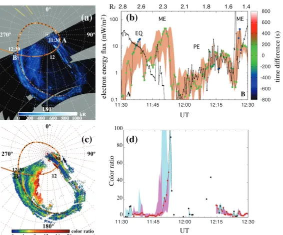
Figure 1. Comparison of the auroral intensity and color ratio observed by ultraviolet spectrograph (UVS) at the Juno magnetic footprint with the corresponding precipitated electron energyﬂux measured by Jupiter Energetic Particle Detector Instrument (JEDI) during the PJ3‐N perijove transit. (a) Polar projection of a global composite image of the unabsorbed H₂auroral emission in the north observed by the UVS spectral imager. System III meridians and parallels are shown as white dotted lines every 10°. The brown dashed line indicates the projected location of the Juno magnetic footprint during the Juno transit. The two short yellow lines point to the solar direction at the beginning and the end of the far ultraviolet (FUV) image. The white dots correspond to hours and the black ones to tens of minutes. (b) JEDI auroral electronﬂux in the loss cone averaged over 30 s is shown by the black dots and solid line. The colored dots indicate the value of the H₂auroral brightness converted into precipitated milliwatt per square meter mapping to the same location as the electrons measured within ±800 s from the corresponding JEDI measurement (see text). The colors indicate the time difference between the two measurements. The shaded brown areas are an estimate of the uncertainty of the brightness associated with a 1,000‐km offset of the nominal magnetic mapping (see text). (c) Global polar projection of the FUV auroral color ratio corresponding to panel (a). (d) FUV color ratio measured along the magnetic foot track. The associated color‐shaded zones indicate the color ratio uncertainty associated with the uncertain magnetic mapping for two different thresholds (0.1 kR in light blue and 0.5 kR in magenta) of the H₂brightness between 125 and 130 nm. The time integration for panels (a) and (c) is identical to the time interval displayed in panels (b) and (d).

(8)

because JEDI does not resolve the loss cone at this altitude. It was followed by a void region followed by the crossing of a bright PS. The peak intensity closely corresponds to the ~100 kR expected from a precipitation of 10 mW/m2. Initially, the JEDIflux exceeded this value of the aurora by a factor of about 4, but the H2 intensity uncertainty inside the brown error zone remains compatible with the JEDI energyflux. Between 15:42 and 15:48, the electronflux dropped by nearly 2 orders of magnitude while the auroral intensity increased. However, during this period, the time difference between the measurements of the two instruments increased from 0 to 336 s. Theflux discrepancy is therefore likely a consequence of the lack of simultaneity when observing a time‐varying PS. In contrast, the two flux determinations are in fairly good agreement after 15:54 in the polar diffuse aurora which is quite stable.

The characteristics of the electron energy and pitch angle distributions are shown in Figure 2. The JEDI elec-tron measurements during the overflight of the bright PS indicate that the upward electron energy flux exceeded the downwardflux by a large factor. This is a common feature that was previously highlighted by Mauk, Haggerty, Paranicas, et al. (2017a); Mauk et al. (2018). The characteristic electron energy of the JEDI spectrum, obtained by dividing the energyflux by the number flux is on the order of 200 keV and remains fairly constant until the end of the period. The JEDI electron energy spectrum, the pitch angle dis-tribution, and the energyflux during Perijove 3‐North (PJ3‐N) between 15:37 and 15:40 were also documen-ted by Mauk et al. (2017a). They identified the signature of two narrow downward acceleration structures peaking at 400 keV during the crossing of the largeflux enhancement visible on panel (b) at 15:37. They showed that, even then, a larger portion of downward energyflux comes from the broadband additions at energies higher and less than the peaked structure. The electron energy spectra quickly evolved into a broad-band distribution without any signature of coherent acceleration and the pitch angle distribution became more isotropic as shown in Figure 2.

Figure 1c shows the polar projection of the color ratio and the magnetic foot track of the Juno in the atmo-sphere on a color scale between 0 and 20. For representation, we choose to saturate values in excess of 20 to this value since they generally correspond to low values of the auroral intensity in the 125‐ to 130‐nm spec-tral window. The void regions are those when the brightness is too low to provide signiﬁcant color ratio values. Figure 1d illustrates the variation of the color ratio measured along the foot track between points A and B. The purple dots correspond to locations when the intensity between 125 and 130 nm was above 0.5 kR, while the black dots set the lower limit to 0.1 kR and are therefore less reliable than the purple dots. The color‐shaded areas show the estimated uncertainty associated with the magnetic mapping for both inten-sity thresholds (0.5 kR in magenta, 0.1 kR in light blue). Some points that have no color‐shaded colored zone because only the intensities at the nominal magnetic footprint location can be extracted from the image. If the brightness in the 125‐ to 130‐nm range is less than 0.1 kR, no color ratio value is given because the denomi-nator of the CR expression gets too small. These two panels indicate that the color ratio remains moderate (<5) during most of the equatorward aurora crossing except for a short time. The polar bright spot is asso-ciated with harder electron precipitation with a color ratio up to ~10. The region of diffuse polar aurora after 15:54 is characterized by a weak UVS signal that does not provide reliable color ratio measurements with the exception of a 3‐min period near 16:11 with a value between 2 and 6.

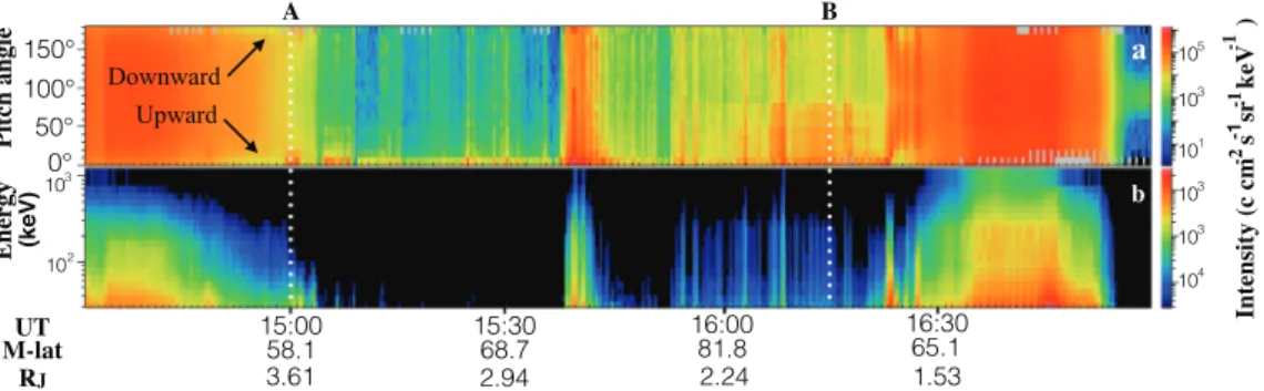
Figure 2. Electron pitch angle (a) and energy distribution above 30 keV (b) measured as a function of time by Jupiter Energetic Particle Detector Instrument while crossing the north auroral region during PJ3 transit in the north. The time period covered by Figure 1b is indicated by the vertical dotted lines. The upward electron intensity (0° to 90° in the north) exceeds the downward intensity. The electrons in the loss cone show a typical broadband energy distribution.

(9)

The intensity polar map (Figure 3a) was collected on 2 February 2017 between 11:33 and 12:28 UT, covering most of the time period discussed here. The period of comparison includes aﬁrst crossing of the equatorward emission including an outer secondary auroral arc in the dawn sector, the dawn ME, regions of weak and brighter diffuse aurora, and a second crossing of the ME in the afternoon sector. During most of the period of concurrent measurements, the time delay between the two measurements remained below 2 min, except for the EQ zone and the second crossing of the ME when it reached ~6 minutes.

The JEDI electronflux in the loss cone is contaminated by the radiation belt contribution until about 11:50 and after 12:25, but a clear signature of auroral electron precipitation is observed as a narrow spike at 11:47, corresponding to the ME (Figure 3b). As for PJ3‐N, a time shift of about 2 min. is observed between the peaks of the two instruments, marginally compatible with the 1,000‐km uncertainty of the magnetic mapping. In any case, the JEDIflux remains much less than the H2auroralflux during most of the transit of the ME structure, although the time difference of the two measurements was less than 2 min. The passage through the void region (from 11:57 to 12:10) is observed by both instruments. During the high‐latitude transit in the diffuse aurora (12:12 to 12:20), the JEDI and UVS energyfluxes are about equal. The emission peak during the second transit through the ME at System III longitudeλIII= 230° before point B is shifted relative to the JEDI spike observed about 2–3 min earlier, probably as a consequence of inaccurate magnetic mapping. The measured H2brightness is then a factor of about 4 less than associated with the JEDIflux peak measured 7 min earlier. A very large color ratio is associated with the dawn crossing of the ME (panels c and d). The inner edge of the diffuse PE at 12:11 also corresponds to a large value of the color ratio. The color ratio only bears a moderate signature of the ME crossing in the afternoon sector. The electron pitch angle distribution indicates that the upwardflux exceeds the downward flux along the field line connecting to the ME and PEs.

(10)

Perijove 5‐North (PJ5‐N) corresponds to a crossing of the auroral region including EQ, a weak signature of the dawn ME, a void sector, diffuse high‐latitude emission and the ME in the dawn sector at λIII~ 170°, as illustrated in Figure 4a. Until about 7:38 UT, Juno was inside the radiation belt as seen in panel (b). Both the UVS and the JEDI energyfluxes subsequently dropped down to the noise level inside a dark void region until ~8:03. The UVS brightness and the associated electron flux increased by about 2 orders of magnitude between 8:00 and 8:12 as the spacecraft moved toward the brighter region at 8:20. During this time interval, the JEDI downwardflux was remarkably less than required to produce to observed UVS intensity, including during periods when the two measurements were made within 30 s between 8:14 and 8:18. Finally, a sharp increase in the JEDIflux reaching 500 mW/m2was detected at 8:28. The JEDI and the UVfluxes were com-parable during the two ME overflights at 7:40 and 8:30.

The color ratio remained less than 5 in the region of equatorward emission between 7:00 and 7:37, raised up to 12 in the ME crossings and 40 in the bright polar region where the UVSﬂux exceeded the in situ electron ﬂux by nearly 2 orders of magnitude.

Interestingly, JADE measurements of the precipitated electronflux between 8:00 and 8:36 described by Ebert et al. (2019) have led to the same conclusion concerning the close agreement with UVS in the ME and the large discrepancy in the polar region between the in situ and the remotely measured auroral electronfluxes. We confirm their observations using the closest UVS measurements in time instead of a single UVS swath.

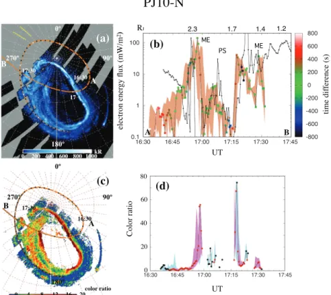
The Perijove 10‐North (PJ10‐N) comparison starts equatorward of the ME when Juno exited the radiation belts in the evening sector, successively crossed the ME at 16:54 UT, a PS between 17:00 UT and 17:15

(11)

UT, a broad JEDI structure from about 17:20 UT till 17:30 UT, with two UV intensity maxima at 17:17 UT and 17:28 UT as shown in Figure 5a. The JEDI peak at 16:54 was offset 4 min earlier than the JEDI peak than the UV peak but of equal magnitude. The strong precipitation at 17:22 was significantly higher than the corresponding UV flux at Juno's magnetic footprint, although the two measurements were made within 100 s. The loss cone was not properly sampled until 17:18, which may explain the lack of correlation near the ME. The UV intensity drop at 17:27 has no counterpart in the JEDIflux. Although the time delay between the two measurements is less than 200 s, this lack of correlation may be a short‐ term temporal variation, a common feature in the active polar region at dusk. The electron pitch angle distribution is bidirectional in the ME, becoming isotropic in the polar diffuse aurora.

The color ratio variation along the orbital path shows large variations between the different auroral regions (panels c and d). A moderate value (CR < 5) is measured in the diffuse EQ before 16:53. A very large value is associated with the crossing of the bright ME a few minutes before 17:00 as seen in panels (c) and (d). However, its exact value is uncertain given the low brightness of the absorbed spectral window. Between 17:20 and 17:27, the JEDI downward electron energyﬂux exceeds by far the H2ﬂux. The color ratio drops to moderate values and rises again, mimicking the FUV intensity variations during this time period.

The Juno magnetic foot track during Perijove 11‐North (PJ11‐N) intersects the equatorward diffuse aurora before 12:50 UT, the bright ME at 13:00 UT in the night sector, a region void of emission between 13:06 and 13:12, and a diffuse PE after 13:10 UT (Figures 6a and 6b).

The JEDI energyflux in the diffuse equatorward aurora is in good agreement with that expected from the intensity observed with UVS. The crossing of the ME shows the same feature as PJ3 and PJ4: a moderate peak in the JEDIflux (12:58 UT) matching the H2auroralflux, followed by a flux drop concurrent with an increase of the UV brightness during the following few minutes, although the time delay remained less below 30 s from 12:57 to 13:04.

(12)

As was observed in PJ5‐N, the flux associated with the UV intensity exceeds the measured JEDI flux by over an order of magnitude at high latitudes (13:10 and 13:20). We note that during this period, the JEDI electron energy remains very low above 40 keV. In the PE, the JEDI electronflux was essentially oriented upward. The downwardflux remained less than the FUV with the exception of two spikes at 13:27 and 13:32. A high energy component (“penetrating radiation”) is observed as described by Paranicas et al. (2018) and Mauk et al. (2018). We note that the magnetic mapping in this region may be less accurate than in other sectors. Figures 6c and 6d show that the color ratio is less than 5 in the EQ and ME, bearing little signature of the ME crossing. Itfluctuates between 5 and 46 in the polar aurora with four peaks concurrent with spikes in the JEDIflux, except at 13:34 when it remains remarkably low in comparison to the preceding 7 min.

4.6. Perijove 7‐South

We now analyze the data collected during two transits in the south polar region. Figure 7a shows that during this southern auroral segment, Junofirst exited the radiation belt and successively crossed magnetic field lines threading the equatorward aurora (2:29 UT), the ME (2:35 UT, patchy in this case), and a PS (2:42 UT) tofinally move into a void polar region near the South Pole. The time delay between the JEDI and UVS data points remained less than 200 s until 2:50 UT and increased afterward.

Theflux peaks corresponding to the crossing of the three regions are almost colocated between JEDI and the UVS (panel b), although they are slightly shifted in time, probably because of residual uncertainties in the JRM09 magneticfield model. The first two UVS and JEDI peaks remained relatively comparable in magni-tude, but the very large electronflux (~200 mW/m2) measured in the PS (PE at 2:42) is up to 20 times larger than the corresponding electronflux exciting the UV aurora at Juno's footprint. During this period, the

(13)

(broadband) upward electronflux along the field lines exceeded the downward electron flux. Although this third peak was associated with a large precipitating electronflux, the FUV color ratio remained moderate (<5). A time delay of ~3–4 min separates the UVS observation of the PS from the crossing of the connecting field line. This time difference may explain the energy flux discrepancy between the two instruments if the UVSfield of view missed a bright polar flare. The dusk polar region is known to exhibit fast and large UV intensity variations such as was described by Waite et al. (2001) and Bonfond et al. (2016). Another possibility is the presence of a downward electricfield slowing down the precipitated electrons between the spacecraft and the atmosphere. This would also explain the moderate value of the correspond-ing color ratio. The protonflux was then quasi‐isotropic, and their energy remained mostly below 100 keV. The fact that downward electric potentials can accompany strong downward electronfluxes (contrary to expectations) was observed by Mauk et al. (2018).

Figures 7c and 7d indicate that, in the equatorward aurora, the color ratio reached a value of 8. In the ME, the electron energy distribution measured by JEDI was quite energetic and the color ratio rose up to about 10. It dropped back to less than 5 at the bright PS location at 12:45. The characteristic energy of the electron precipitation in the JEDI energy range obtained by dividing the energyflux by the number flux remained quasi constant at ~250 keV between 2:35 and 2:45. This constancy is in contrast with the FUV color ratio, which exhibits a significant decrease during this time interval. The drop of the mean energy of the electrons reaching the atmosphere (associated with the low color ratio) would be compatible with the assumption of a downward electricfield below Juno that was flying at an altitude between 0.7 and 0.9 R_Jat this period.

4.7. Perijove 12‐South

The Juno trajectory during this comparison (Figure 8a) maps to the equatorward emission nearλIII= 180° at 10:42 UT, to a broad ME region (on the right‐hand side of the arrow labeled PE in panel (b) from 10:45 to 10:58 UT followed by diffuse PE up to point B. As seen in panel (b), during the ME crossing JEDI measured the highest precipitated energyﬂux (325 mW/m2) measured among all seven cases described in this study.

Figure 7. Same as Figure 1 but for PJ7‐S. The polar projections (panels a and c) represent the southern aurora as would be seen through the planet from above the North Pole.

(14)

The electron pitch angle distribution was bidirectional with an upward flux exceeding the downward electron flux. The (broadband) JEDI electron distribution in the loss cone was very energetic (mean energy above 200 keV in the JEDI energy range). From 10:45 until point B, less than 200 s separated the JEDI and UVS measurements. The peak JEDIflux in the ME exceeded the UVS flux by up to a factor of 10 but the situation inverted after 10:58. In the polar diffuse emission the equivalent UVS powerflux remained almost continuously larger than the JEDI measurements including times when the two observations were concurrent within less than 30 s.

In this case, the close simultaneity of several UVS and JEDI measurements strongly suggests that the differ-ence in energyﬂux and mean energy between the two levels (Juno and the atmosphere) is real and that downward acceleration of the auroral electron below the spacecraft is taking place. This scenario is all the more likely that Juno was far above the atmosphere (1.5 to 2.2 RJ) during these coincident measurements. The color ratio (panels c and d) exhibits a peak up to 10, coincident with the maximum UVS intensity in the ME, followed by drop below 5. Poleward of the ME, the color ratio is more structured than the H2brightness, ranging from about 3 to 24 (red data points) between 11:00 and 11:25 uncorrelated with the UVS brightness at Juno's footprint. As for Perijove 7‐South (PJ7‐S), the JEDI characteristic energy remained close to 150 keV between 11:00 and 11:30, in contrast to the strong variations observed in the FUV color ratio.

5. Discussion

In this section, we discuss some of the main features from this multiorbit comparison of the in situ electron precipitation with the auroral brightness.

5.1. Magnetic Field Mapping

Each perijove sequence of observations is different in location, System III longitude, local time, and solar wind condition. However, several general conclusions may be drawn from the comparison of the morphol-ogy of the images of the H2auroral emissions images by UVS, the color ratio along the Juno magnetic foot-print, and the precipitated electron energyﬂux measured by the JEDI instrument. We ﬁrst examine features

(15)

common to some of the seven cases examined in this study. In a second step, we discuss possible interpreta-tion of the main features deduced from these comparisons.

As mentioned before, afirst feature common to all seven cases is the generally good match between the timing (and localization) of the auroral structures along the Juno magnetic track and the corresponding characteristics of the electron precipitation measured on board Juno. The morphological features are remarkably close to those measured in the electronflux by JEDI. This mapping along the magnetic field lines is considerably more accurate than was provided by earlier B‐field models before Juno's magnetic field investigation measurements. Mapping uncertainties were illustrated by Bonfond et al.'s (2017) Figure 3 where they compared the UVS brightness along Juno's foot track using the VIP4 (Connerney et al., 1998) or VIPAL (Hess et al., 2011) models. Examples of this agreement are the crossings of the ME during Perijove 4‐North (PJ4‐N), PJ5‐N, PJ7‐S, PJ10‐N, and PJ12‐S. Similarly, the penetration of Juno into regions of intense polar precipitation is closely coincident with the crossing of PSs or diffuse aurora observed dur-ing PJ3‐N, PJ4‐N, PJ7‐S, PJ10‐N, and PJ11‐N. This coincidence of features observed with JEDI and UVS confirms the quality of the JRM09 magnetic field and its ability to map the magnetic field line between Juno and the Jovian upper atmosphere.

5.2. Color Ratio

The color ratio associated with the ME crossing is generally high (10 or more, corresponding to the red regions in panels (c) when the aurora is bright, compared to the other auroral features. This is the case of PJ4‐N, PJ5‐N, PJ7‐S, and PJ12‐S. A remarkable exception is PJ11‐N at 13:00 when the color ratio at the footprint of the ﬁeld line connecting to Juno barely showed a small enhancement and remained below 5.

In the polar regions, UVS observations show regions of high color ratios that are not necessarily associated with bright auroral emission, especially in the Northern Hemisphere. As was described in section 4, these regions are sometimes associated with a precipitated energyﬂux at Juno's altitude that is largely insufﬁcient to produce the observed H2intensity.

The global morphology of the color ratio distribution were previously observed by Gérard et al. (2014, 2016) and Gustin et al. (2016) in spectral images that were obtained from spatial scans of the polar regions during latitudinal slews of the HST. Their mainﬁndings are conﬁrmed and, more importantly, observed by Juno both on the dayside and the nightside of the planet.

5.3. Comparison of UVS and JEDI Electron Energy Fluxes

Comparisons of the electron energyflux associated with the H2intensity and the downwardflux measured by Juno inside the loss cone along the same magneticfield line reveal possible modifications of the electron energy and/or pitch angle distributions between Juno and the atmosphere. This can also bear the signature of electron acceleration or deceleration between the spacecraft and the aurora. Therefore, the ratio between the H2‐derived auroral flux and the in situ measurements is a signature of processes occurring between the two altitude regimes. As for the color ratio, wefirst summarize the characteristics of the JEDI‐UVS relation in the EQ, ME, and PE observed during the seven Juno transits.

When available, the UVS and JEDI energyfluxes are in reasonably good agreement in the EQ (except PJ3‐ N), although the radiation belts sometimes contaminate the JEDI measurements. Radioti et al. (2009) showed that the auroral emission equatorward of the ME was excited by energetic electrons scattered into the loss cone as a result of their interaction with whistler waves. Bhattacharya et al. (2005) had suggested that wave‐particle interactions in a broad region of the magnetosphere at distances ~10 to 25 RJfrom the pla-net, exceeding by far the altitude of the Juno, could lead to electron precipitation into the ionosphere. Consequently, a reasonable agreement between the JEDI electronflux and the auroral intensity is expected in this region, in the absence of any further process modifying the electronflux characteristics. The shape of the electron energy spectra measured on board Galileo at distances mapping to the diffuse equatorward emission suggests that the mean electron energy is less than 100 keV.

The JEDI‐UVS flux comparison for the ME is more complex. PJ3‐N, PJ10‐N, and PJ11‐N show examples of electronflux‐auroral brightness structures where the peak of the JEDI energy flux is comparable to the cor-responding UVflux but is significantly narrower and drops by more than an order of magnitude faster than

(16)

the corresponding H2‐derived energy flux. In contrast, the PJ5‐N ME crossing shows no excess H2auroral emission, in agreement with the comparison with the JADE measurements by Ebert et al. (2019). PJ7‐S shows some excess JEDIflux at 2:34 when crossing the field lines threading the ME. In all cases, except PJ11‐N where the main oval was disrupted in the region where Juno crossed the ME, the crossing of the main UV emission is associated with a significant increase of the color ratio.

In the high‐latitude aurora inside the ME, a deficit of precipitated energy flux at Juno's altitude was observed when Juno was crossing polar diffuse emissions during PJ5 and PJ11 in the north and PJ7 and PJ12 in the south. In contrast, the JEDIflux agrees well with the diffuse polar auroral brightness observed in PJ3‐N and PJ4‐N. The color ratio at high latitudes also exhibits a high color ratio in regions of moderate auroral brightness and electron energyflux. This feature is compatible with the assumption that, in these cases, Juno wasflying above most of the (probably extended) downward electron acceleration region, that is, at an altitude of 0.3–1.2 R_J. In this scenario, the energization processes would generate bidirectional electron beams. However, it is also necessary to explain that (1) the upward electronflux may significantly exceed the planetwardflux at Juno's altitude and (2) the downward flux measured by JEDI may be less than required to produce the aurora observed at the magnetic footprint of the spacecraft.

Traditionally, wave‐particle interaction such as Alfvénic acceleration and potential drop acceleration are two prominent mechanisms for auroral acceleration. The question of the altitude of the electron acceleration region leading to the ME was discussed by Cowley and Bunce (2001), in the frame of the global current cir-cuit andfield‐aligned acceleration. They calculated the minimum jovicentric radial distance of the top of the acceleration region and the“vertical” extension of this region. For the current sheet model, they found that acceleratedfield‐aligned electron beams would extend to an altitude at least 3 RJ, where the electron beams would form an extended source of cyclotron radio emission. For the dipolefield approximation, they claimed that the acceleration region may form at lower altitudes, on the order of 0.5 RJabove the aurora (Cowley et al., 2003, 2017). These values were found quasi‐independent of the ionospheric Pedersen conductivity. In this study, Juno wasflying between 0.3 and 1.7 RJwhen crossing thefield line connecting to the ME. Care must be exercised in that the observations made by Juno in the vicinity of the auroral acceleration regions do not comport with expectations based on the global current circuit model. Acceleration is predo-minantly broadband and generally not associated with inverted‐V structures and potential drops. It is even found that strong downward electron acceleration can accompany strong downward electron potentials, the opposite situation from that expected from the global current circuit model (Mauk et al., 2018). Connerney et al. (2017) and Kotsiaros et al. (2019) reported that magneticfield perturbations indicate that the parallel electric currents arefilamentary and weaker than anticipated.

In contrast to electrostatic acceleration, Hess et al. (2010) discussed the location where the electrons causing the Io footprint are energized assuming that the acceleration is generated by the parallel electricfield in the region of the peak of inertial Alfvén waves. At Jupiter, this process is efficient where the electrons are fast enough to escape the strong oscillating parallel electricfield before it reverses its phase so that bidirectional beams of energetic electrons are created. They found that it is located between 0.5 and 1.5 RJabove the iono-sphere. The lower altitude corresponds to the dipole approximation of the magneticfield and a cold iono-spheric plasma. A more detailed B‐field model with a warmer ionospheric plasma (heated by the aurora) locates the acceleration region at the higher altitude. Although these developments were made in the context of acceleration of the electrons producing the Io footprint, these results may also apply to the ME and the PE. In summary, according to current ideas about electron energization processes, the bulk of the acceleration takes place at an altitude between ~0.5 and 1.5 RJ. This range is within the altitudes of the ME and the PE crossings analyzed in this study. Therefore, it is reasonable to assume that, depending on the ionospheric plasma conditions and the magnitude of the magneticfield, Juno may fly below, inside, or above a vertically extended region of electron acceleration during the times of these comparisons. The downward electronflux at Juno's altitude is only expected to be comparable to theflux interacting with the atmosphere if no accel-eration occurs along thefield line below Juno's altitude. If Juno is located above most of this region, JEDI measures a downward electronflux that is less than the flux reaching the atmosphere. In any case, condi-tions of brighter aurora than expected from JEDI measurements of energetic electrons in the loss cone imply an additional acceleration process below the Juno spacecraft. In some events, we alsofind strong upward electron flux coexisting with the bright aurora, which implies the coexistence of both upward and

(17)

downward acceleration. We therefore speculate that potential drop and wave‐particle processes may coexist below Juno. The wave‐particle interaction strongly energizes electrons, while downward electric ﬁeld pre-vents the portion of electrons with parallel energies less than the potential drop deceleration from precipitat-ing into the ionosphere and atmosphere. This would also lead to the observed increase of the lower‐energy upward electronﬂux.

6. Conclusion and Summary

We have described seven cases of quasi‐simultaneous measurements of the electron energy ﬂux associated with the FUV auroral brightness and color ratio at Juno's magnetic footprint together with in situ energetic (>20 keV) precipitating electrons. Five observations were made in the Northern Hemisphere and two were collected in the South. The in situ electron measurements were made at distances ranging from about 0.3 to 1.8 RJabove the aurora. The comparison of the data from the two instruments shows regions of close agreement and strong disagreement between the energy ﬂuxes at the spacecraft. In brief, we conclude the following:

• We note that the JRM09 magnetic field model maps well the magnetic field line connecting Juno to the Jovian upper atmosphere. This is a significant improvement for the combined study of in situ and remo-tely sensed Jovian aurora compared to earlier B‐field models such as VIP4 and VIPAL, less accurate at short distances from the planet.

• The intensity of the diffuse emission located equatorward of the main oval is generally in fair agreement with the JEDI downward energyﬂux. This agreement may be expected on the basis of earlier studies indi-cating that distant wave‐electron interaction cause electron pitch angle scattering into the loss cone. It is thus expected that the bulk of the acceleration is generated at a distance beyond the altitude of Juno dur-ing the crossdur-ing of this region.

• The energy flux inferred from the main auroral emission is sometimes well matched by the observed JEDI electron energyflux or at times is found to exceed the brightness expected from the in situ measurements. These two cases imply that Juno may beflying under or above, respectively, the acceleration region dur-ing the main oval crossdur-ing (altitude ~ 0.3–1.7 R_J). However, comparison of the detailed structure indicates that electronflux precipitation at Juno's altitude may also appear less extended in latitude and weaker than the UV arc.

• The high value of the color ratio usually associated with the ME is in good agreement with earlier (HST) observations and compatible with predictions based onﬁeld‐aligned acceleration in a global current cir-cuit. However, the shape of the measured electron spectrum indicates that stochastic wave‐particle accel-eration provides the bulk of the energy needed to match the observed brightness and color ratio. • A deﬁcit of precipitating energetic electrons relative to the UV brightness has been observed inside the ME

(“polar cap”) on several but not all occasions. The FUV color ratio therein may reach very large values. Both results indicate that an efﬁcient energization process may occur between Juno (altitude ~0.3–1.2 RJ) and the aurora.

• Both wave‐particle and ﬁeld‐aligned acceleration models predict that the electron acceleration region extends between 0.5 and 1.5 RIabove the aurora. This range of altitudes is compatible with our reported observations of coincident relatively low electron precipitation and large color ratio in the polar regions.

Appendix A: Sources of UVS Intensity Uncertainties

The sources of uncertainties in the evaluation of the auroral electronﬂux associated with the UVS observa-tions belong to two categories: (i) systematic errors linked to the conversion of the count rate measured into brightness and precipitated electron energyﬂux and (ii) random errors depending on the strength of the sig-nal, the instrument response and the background level. These contributions are discussed below.

Systematic Error

To calibrate the UVS instrument, bright hot stars observations are used to measure the effective area among other instrumental characteristics. Data are coadded from many spins to build up exposure times. Calibration observations were made during the commissioning phase and are performed regularly near apojove to check for possible aging of the instrument. These observations were made during a total integration time on a star of ~4 s for the wide slit and 0.6 s for the narrow slit, when typical observations of 2.5 hr are coadded. The absolute

(18)

effective area is used to convert measured counts/pixels into physical units such as kiloRayleighs. It is deter-mined by observing bright hot stars and dividing the measuredﬂux by the calibrated ﬂux given by IUE or Hubble observations. In the regions of the H2spectrum used for this study, the uncertainty on the effective area is estimated ~16%, in fair agreement with the ground‐based calibration (Hue et al., 2019).

The conversion of the brightness into the total unabsorbed H2emission in the Lyman and Werner bands is described in section 2. This step carries only weak uncertainties since the fraction emitted in a given spectral window is known and varies only very weakly with temperature. This was demonstrated by numerical tests and comparisons between synthetic H2spectra and laboratory spectra produced by electron impact on ground state H2molecules (Gustin et al., 2012). The factor between the total H2unabsorbed intensity and the electron energyflux interacting with the atmosphere is based on the results of model simulations of elec-tron transport in a H2atmosphere. Several methods have been used giving slightly different results. Gérard and Singh (1982) obtained a value of 10.6 kR of Lyman and Werner bands per incident milliwatt per square meter for a pure H2atmosphere based a continuous slow down approximation. Waite et al. (1983) derived a value of 9.2 kR/mW·m−2using a two‐stream approach. Both studies assumed low primary electron energy of a few kiloelectron volts. The magnitude of the excitation cross section for electron impact on H2depends on the electron energy. However, the excitation of the B and C singlet states is largely caused by impact of ondary (lower energy) electrons. Grodent et al. (2001) used the energy dependence of the excitation cross sec-tions for the B and C states determined by Liu et al. (1998) claimed to be accurate to better than 10%, with a negligible temperature variation of 0.7% at 100 eV between 500 and 1000 K for the Lyman bands. Their pri-mary electron energy spectrum was composed of the superposition of three Maxwellian distributions extend-ing from 11 eV to 500 keV to model a discrete aurora and obtained an efficiency of 10.0 kR/mW·m−2. For a diffuse, less energetic precipitation, the calculated efficiency was 9.7 kR/mW·m−2, also quite close to earlier determinations. We adopt the standard value of 10 kR of Lyman and Werner band emission for a 1 mW/m2 electron precipitation, midway between the values published in the literature. The uncertainty on the preci-pitated from the efficiency calculated with different models is ~7%. The dependence of auroral emission effi-ciency with the pitch angle distribution was found to be small, on the order of 2%, between monodirectional and isotropic pitch angle distributions. Combining the three sources of errors, we estimate the uncertainty on the scaling factor on the order of 12%, that is, 10±1.2 kR/mW·m−2.

Random Error

Aﬁrst source is the shot noise associated with the limited number of photon events detected during the time interval of the measurements. Its standard deviation is equal to the reciprocal square root of the number of detected events inside the spectral range considered during a given observation. During each spacecraft spin, a given point on the planet is seen during∼17 and ∼2 ms through the wide and narrow slits, respectively. As mentioned is section 3, we use the brightness measured during the spin closest in time to the JEDI measure-ments. The auroral brightness is averaged over a 400‐km radius circle. This area includes a variable number of pixels depending on Juno's altitude. For example, if we integrate over 25 pixels, one count/pixel is pro-duced by approximately 10 kR of H2emission. Therefore, an average 10 kR signal corresponds to a measure-ment of 25 counts. The shot noise level in this case is equal toﬁve counts and the associated uncertainty is 5/25 or 20%. Similarly, a 100‐kR intensity is associated with a 6.5% noise level and 1,000 kR to 2%.

Part of the random uncertainty stems from the subtraction of the background noise. The correction consists in subtracting the background signal generated by the interaction of penetrating energetic particles with the MCP detector. For each observation, the background subtraction is made by using the counts recorded in a region of the detector located between pixels 345 and 550 along the detector X axis (~59.7 to 80.9 nm) and between pixels 20 and 255 in the direction along the slit. This region is essentially void of photon counts because of the very low effective area (Hue et al., 2018). Counts observed in this“dark” sector of the detector are thus essentially due to energetic electron impacts. Observations carried out within the radiation belts have been made to determine the relative response of the different pixels of the detector to penetrating radia-tions. This response is used to evaluate and subtract the particle noise in the illuminated parts of the detec-tor, based on the count rate observed in the dark sector. This contribution and its associated uncertainty can vary very rapidly, within time scales down to 0.1 s (Bonfond et al., 2018) with several factors such as the loca-tion and the orientaloca-tion of the spacecraft and the prevailing magnetospheric condiloca-tions. As an example, we consider a particularly unfavorable case for which the background level is on the same order as the photon