HAL Id: hal-01313005
https://hal.archives-ouvertes.fr/hal-01313005v3
Preprint submitted on 26 Oct 2017
HAL is a multi-disciplinary open access
archive for the deposit and dissemination of sci-entific research documents, whether they are pub-lished or not. The documents may come from teaching and research institutions in France or abroad, or from public or private research centers.
L’archive ouverte pluridisciplinaire HAL, est destinée au dépôt et à la diffusion de documents scientifiques de niveau recherche, publiés ou non, émanant des établissements d’enseignement et de recherche français ou étrangers, des laboratoires publics ou privés.
Public Domain
To cite this version:
Romain Brault, Florence d’Alché-Buc. Random Fourier Features for Operator-Valued Kernels. 2017. �hal-01313005v3�
Random Fourier Features for Operator-Valued Kernels
Brault Romain [email protected]
LTCI
T´el´ecom ParisTech
Paris, 46 rue Barrault, France Universit´e Paris-Saclay
Florence d’Alch´e-Buc [email protected]
LTCI
T´el´ecom ParisTech
Paris, 46 rue Barrault, France Universit´e Paris-Saclay
Editor: John Doe
Abstract
Many problems in Machine Learning can be cast into vector-valued functions approximation. Operator-Valued Kernels Operator-Valued Kernels and vector-valued Reproducing Kernel Hilbert Spaces provide a theoretical and versatile framework to address that issue, extending nicely the well-known setting of scalar-valued kernels. However large scale applications are usually not affordable with these tools that require an important computational power along with a large memory capacity. In this paper, we aim at providing scalable methods that enable efficient regression with Operator-Valued Kernels. To achieve this goal, we extend Random Fourier Features, an approximation technique originally introduced for translation-invariant scalar-valued kernels, to translation-invariant Operator-Valued Kernels. We develop all the machinery in the general context of Locally Compact Abelian groups, allowing for coping with Operator-Valued Kernels. Eventually, the provided approximated operator-valued feature map converts the nonparametric kernel-based model into a linear model in a finite-dimensional space.
Keywords: Random Fourier Feature, Operator-Valued Kernel
1. Introduction
Learning vector-valued functions is key to numerous tasks in Machine Learning such as multi-label classification, multi-task regression, vector field learning. Among the different families of tools that currently allow to address multiple output prediction, Operator-Valued Kernel methods (Micchelli and Pontil, 2005; Carmeli et al., 2010; Kadri et al., 2010; Brouard et al., 2011; ´Alvarez et al., 2012) benefit from a well founded theoretical background while being flexible enough to handle a large variety of problems. In a few words, Operator-Valued Kernels extend the classic scalar-valued kernels to functions with values in output Hilbert spaces. As in the scalar case, Operator-Valued Kernels (OVKs) are used to build Reproducing Kernel Hilbert Spaces (RKHS) in which representer theorems apply as for ridge regression or other appropriate loss functional. In these cases, learning a model in
the RKHS boils down to learning a function of the form 𝑓 (𝑥) = ∑︀𝑁
𝑖=1𝐾(𝑥, 𝑥𝑖)𝛼𝑖 where 𝑥1, . . . , 𝑥𝑁 are the training input data and each 𝛼𝑖, 𝑖 = 1, . . . , 𝑁 is a vector of the output space 𝒴, and each 𝐾(𝑥, 𝑥𝑖) is an operator on 𝒴.
However, OVKs suffer from the same drawbacks as classic (scalar-valued) kernel machines: they scale poorly to large datasets because they are exceedingly demanding in terms of memory and computations.
In this paper, we propose to keep the theoretical benefits of working with OVKss while providing efficient implementations of learning algorithms. To achieve this goal, we study feature map approximations ̃︀𝜑 of OVKs that allow for shallow architectures, namely the product of a (nonlinear) operator-valued feature ̃︀𝜑(𝑥) and a parameter vector 𝜃 such that
̃︀
𝑓 (𝑥) = ̃︀𝜑(𝑥)*𝜃.
To approximate OVKs, we extend the well-known methodology called Random Fourier Features (RFFs) (Rahimi and Recht, 2007; Le et al., 2013; Yang et al., 2015b; Sriperumbudur and Szabo, 2015; Bach, 2015; Sutherland and Schneider, 2015; Rudi et al., 2016) so far developed to speed up scalar-valued kernel machines. The RFF approach linearizes a shift-invariant kernel model by generating explicitly an approximated feature map ˜𝜙. RFFs has been shown to be efficient on large datasets (Rudi et al., 2016). Additionally, it has been further improved by efficient matrix computations such as (Le et al., 2013, “FastFood”) and (Felix et al., 2016, “SORF”), that are considered as the best large scale implementations of kernel methods, along with Nystr¨om approaches proposed in Drineas and Mahoney (2005). Moreover thanks to RFFs, kernel methods have been proved to be competitive with deep architectures (Lu et al., 2014; Dai et al., 2014; Yang et al., 2015a).
1.1 Outline and contributions
The paper is structured as follow. In Section 2 we recall briefly how to obtain RFFs for scalar-valued kernels and list the state of the art implementation of RFFs for large scale kernel learning. Then we define properly Operator-Valued Kernels, give some important theorems and properties used throughout this paper before given a non exhaustive list of problem tackled with OVKs.
Then we move on to our contributions. In Section 3 we propose an RFF construction from 𝒴-Mercer shift invariant OVK that we call Operator-valued Random Fourier Feature (ORFF). Then we study the structure of a random feature corresponding to an OVK (without having to specify the target kernel). Eventually we use the framework used to construct ORFFs to study the regularization properties of OVKs in terms of Fourier Transform.
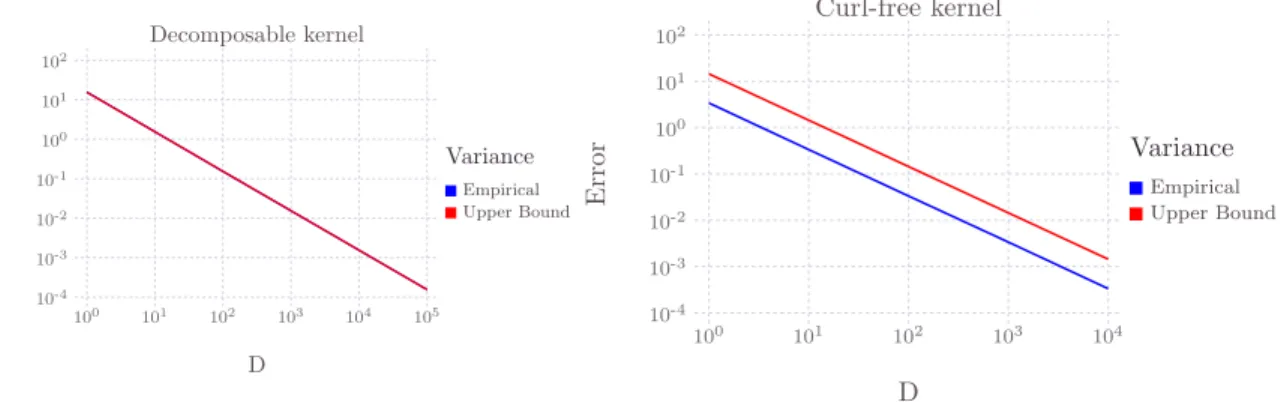
In Section 4 we assess theoretically the quality of our ORFF: we show that the stochastic ORFF estimator converges with high probability toward the target kernel and derive convergence rates. We also give a bound on the variance of the approximated OVK constructed from the corresponding ORFF.
In Section 5 we focus on Ridge regression with OVKs. First we study the relationship between finding a minimizer in the VV-RKHS induce by a given OVK and the feature
induced by the corresponding ORFF. Then we define a gradient based algorithm to tackle Ridge regression with ORFF, show how to obtain an efficient implementation and study its complexity.
Eventually we end this paper by some numerical experiments in Section 6 on toy and real datasets before giving a general conclusion in Section 7.
2. Background
Notations used throughout this paper are summarized in Table 1. 2.1 Random Fourier Feature maps
The Random Fourier Features methodology introduced by Rahimi and Recht (2007) provides a way to scale up kernel methods when kernels are Mercer and translation-invariant. We view the input space 𝒳 as the group R𝑑 endowed with the addition law. Extensions to other group laws such as Li et al. (2010) are described in Subsection 3.2.2 within the general framework of operator-valued kernels.
Denote 𝑘 : R𝑑× R𝑑→ R a positive definite kernel (Aronszajn, 1950) on R𝑑. A kernel 𝑘 is said to be shift-invariant or translation-invariant for the addition if for all (𝑥, 𝑧, 𝑡) ∈(︀
R𝑑)︀3 we have 𝑘(𝑥 + 𝑡, 𝑧 + 𝑡) = 𝑘(𝑥, 𝑧). Then, we define 𝑘0 : R𝑑 → R the function such that 𝑘(𝑥, 𝑧) = 𝑘0(𝑥 − 𝑧). The function 𝑘0 is called the signature of kernel 𝑘. If 𝑘0 is a continuous function we call the kernel “Mercer”. Then, Bochner’s theorem (Folland, 1994) is the theoretical result that leads to the Random Fourier Features.
Theorem 1 (Bochner’s theorem)
Any continuous positive-definite function (e. g. a Mercer kernel) is the Fourier Transform of a bounded non-negative Borel measure.
It implies that any positive-definite, continuous and shift-invariant kernel 𝑘, have a continuous and positive-definite signature 𝑘0, which is the Fourier Transform ℱ of a non-negative measure 𝜇. We therefore have the 𝑘(𝑥, 𝑧) = 𝑘0(𝑥 − 𝑧) =
∫︀
R𝑑exp(−i⟨𝜔, 𝑥 − 𝑧⟩)𝑑𝜇(𝜔) = ℱ [𝑘0] (𝜔). Moreover 𝜇 = ℱ−1[𝑘0]. Without loss of generality, we assume that 𝜇 is a probability measure, i. e. ∫︀
R𝑑𝑑𝜇(𝜔) = 1 by renormalizing the kernel since ∫︀
R𝑑𝑑𝜇(𝜔) = ∫︀
R𝑑exp(−i⟨𝜔, 0⟩)𝑑𝜇(𝜔) = 𝑘0(0). and we can write the kernel as an expectation over a probability measure 𝜇. For all 𝑥, 𝑧 ∈ R𝑑
𝑘0(𝑥 − 𝑧) = E𝜔∼𝜇[exp(−i⟨𝜔, 𝑥 − 𝑧⟩)] .
Eventually, if 𝑘 is real valued we only write the real part, 𝑘(𝑥, 𝑧) = E𝜔∼𝜇[cos⟨𝜔, 𝑥 − 𝑧⟩] = E𝜔∼𝜇[cos⟨𝜔, 𝑧⟩ cos⟨𝜔, 𝑥⟩ + sin⟨𝜔, 𝑧⟩ sin⟨𝜔, 𝑥⟩]. Let ⨁︀𝐷𝑗=1𝑥𝑗 denote the 𝐷𝑑-length column vector obtained by stacking vectors 𝑥𝑗 ∈ R𝑑. The feature map 𝜙 : R̃︀
𝑑→ R2𝐷 defined as (1) ̃︀ 𝜙(𝑥) = √1 𝐷 𝐷 ⨁︁ 𝑗=1 (︃ cos ⟨𝑥, 𝜔𝑗⟩ sin ⟨𝑥, 𝜔𝑗⟩ )︃ , 𝜔𝑗 ∼ ℱ−1[𝑘0] i. i. d.
is called a Random Fourier Feature (map). Each 𝜔𝑗, 𝑗 = 1, . . . , 𝐷 is independently and identically sampled from the inverse Fourier transform 𝜇 of 𝑘0. This Random Fourier Feature
Table 1: Mathematical symbols and their signification (part 1).
Symbol Meaning
𝑒 ∈ 𝒳 The neutral element of the group 𝒳 .
𝛿𝑖𝑗 Kronecker delta function. 𝛿𝑖𝑗 = 0 if 𝑖 ̸= 𝑗, 1 otherwise. ̂︀
𝒳 The Pontryagin dual of 𝒳 when 𝒳 is a LCA group. ⟨·, ·⟩𝒴 The canonical inner product of the Hilbert space 𝒴.
‖·‖𝒴 The canonical norm induced by the inner product of the Hilbert space 𝒴. ℱ (𝒳 ; 𝒴) Topological vector space of functions from 𝒳 to 𝒴.
𝒞(𝒳 ; 𝒴) The topological vector subspace of ℱ of continuous functions from 𝒳 to 𝒴. ℒ(ℋ; 𝒴) The space bounded linear operator from a Hilbert space ℋ to a Hilbert
space 𝒴.
‖·‖𝒴,𝒴′ The operator norm ‖Γ‖𝒴,𝒴′ = sup‖𝑦‖
𝒴=1‖Γ𝑦‖𝒴′ for all Γ ∈ ℒ(𝒴, 𝒴 ′) ℳ𝑚,𝑛(K) The space of matrices of size (𝑚, 𝑛).
ℒ(𝒴) The space of bounded linear operator from a Hilbert space 𝒴 to itself. ℒ+(𝒴) The space of non-negative bounded linear operator from a Hilbert space ℋ
to itself.
ℬ(𝒳 ) Borel 𝜎-algebra on a topological space 𝒳 . Leb(𝒳 ) The Lebesgue measure of 𝒳 .
Haar(𝒳 ) A Haar measure of 𝒳 .
Pr𝜇,𝜌(𝒳 ) A probability measure of 𝒳 whose Radon-Nikodym derivative (density) with respect to the measure 𝜇 is 𝜌.
ℱ [·] The Fourier Transform operator.
𝐿𝑝(𝒳 , 𝜇; 𝒴) The Banach space of ‖·‖𝑝𝒴 (Bochner)-integrable function from (𝒳 , ℬ(𝒳 ), 𝜇) to 𝒴 for 𝑝 ∈ R+. 𝐿𝑝(𝒳 , 𝜇, R) := 𝐿𝑝(𝒳 , 𝜇) and 𝐿𝑝(𝒳 , 𝜇, R) = 𝐿𝑝(𝒳 , 𝜇). ⨁︀𝐷
𝑗=1𝑥𝑖 The direct sum of 𝐷 ∈ N vectors 𝑥𝑖’s in the Hilbert spaces ℋ𝑖. By definition ⟨⨁︀𝐷 𝑗=1𝑥𝑗, ⨁︀𝐷 𝑗=1𝑧𝑗⟩ = ∑︀𝐷 𝑗=1⟨𝑥𝑗, 𝑧𝑗⟩ℋ𝑖. ‖·‖𝑝 The 𝐿𝑝(𝒳 , 𝜇, 𝒴) norm. ‖𝑓 ‖𝑝𝑝 := ∫︀ 𝒳‖𝑓 (𝑥)‖ 𝑝 𝒴𝑑𝜇(𝑥). When 𝒳 = N*, 𝒴 ⊆ R and 𝜇 is the counting measure and 𝑝 = 2 it coincide with the Euclidean norm ‖·‖2 for finite dimensional vectors.
‖·‖∞ The uniform norm ‖𝑓 ‖∞= ess sup { ‖𝑓 (𝑥)‖𝒴 | 𝑥 ∈ 𝒳 } = lim𝑝→∞‖𝑓 ‖𝑝. |Γ| The absolute value of the linear operator Γ ∈ ℒ(𝒴), i. e. |Γ|2 = Γ*Γ. Tr [Γ] The trace of a linear operator Γ ∈ ℒ(𝒴).
‖·‖𝜎,𝑝 The Schatten 𝑝-norm, ‖Γ‖𝑝𝜎,𝑝= Tr [|Γ|𝑝] for Γ ∈ ℒ(𝒴), where 𝒴 is a Hilbert space. Note that ‖Γ‖𝜎,∞ = 𝜌(Γ) ≤ ‖Γ‖𝒴,𝒴.
< “Greater than” in the Loewner partial order of operators. Γ1 < Γ2 if 𝜎(Γ1− Γ2) ⊆ R+.
∼
map provides the following Monte-Carlo estimator of the kernel: ̃︀𝑘(𝑥, 𝑧) =𝜙(𝑥)̃︀ *𝜙(𝑧). Using̃︀ trigonometric identities, Rahimi and Recht (2007) showed that the same feature map can also be written (2) ˜ 𝜙(𝑥) = √︂ 2 𝐷 𝐷 ⨁︁ 𝑗=1 (︁ cos(⟨𝑥, 𝜔𝑗⟩ + 𝑏𝑗) )︁ ,
where 𝜔𝑗 ∼ ℱ−1[𝑘0], 𝑏𝑗 ∼ 𝒰 (0, 2𝜋) i. i. d.. The feature map defined by Equation 1 and Equation 2 have been compared in Sutherland and Schneider (2015) where they give the condition under wich Equation 1 has lower variance than Equation 2. For instance for the Gaussian kernel, Equation 1 has always lower variance. In practice, Equation 2 is easier to program. In this paper we focus on random Fourier feature of the form given in Equation 1.
The dimension 𝐷 governs the precision of this approximation, whose uniform convergence towards the target kernel can be found in Rahimi and Recht (2007) and in more recent papers with some refinements proposed in Sutherland and Schneider (2015) and Sriperumbudur and Szabo (2015). Finally, it is important to notice that Random Fourier Feature approach only requires two steps before the application of a learning algorithm: (1) define the inverse Fourier transform of the given shift-invariant kernel, (2) compute the randomized feature map using the spectral distribution 𝜇. Rahimi and Recht (2007) show that for the Gaussian kernel 𝑘0(𝑥 − 𝑧) = exp(−𝛾‖𝑥 − 𝑧‖22), the spectral distribution 𝜇 is a Gaussian distribution. For the Laplacian kernel 𝑘0(𝑥 − 𝑧) = exp(−𝛾‖𝑥 − 𝑧‖1), the spectral distribution is a Cauchy distribution.
2.1.1 Extensions of the RFF method
The seminal idea of Rahimi and Recht (2007) has opened a large literature on random features. Nowadays, many classes of kernels other than translation invariant are now proved to have an efficient random feature representation. Kar and Karnick (2012) proposed random feature maps for dot product kernels (rotation invariant) and Hamid et al. (2014) improved the rate of convergence of the approximation error for such kernels by noticing that feature maps for dot product kernels are usually low rank and may not utilize the capacity of the projected feature space efficiently. Pham and Pagh (2013) proposed fast random feature maps for polynomial kernels.
Li et al. (2010) generalized the original RFF of Rahimi and Recht (2007). Instead of computing feature maps for shift-invariant kernels on the additive group (R𝑑, +), they used the generalized Fourier transform on any locally compact abelian group to derive random features on the multiplicative group (R𝑑, *). In the same spirit Yang et al. (2014b) noticed that an theorem equivalent to Bochner’s theorem exists on the semi-group (R𝑑>0, +). From this they derived “Random Laplace” features and used them to approximate kernels adapted to learn on histograms.
To speed-up the convergence rate of the random features approximation, Yang et al. (2014a) proposed to sample the random variable from a quasi Monte-Carlo sequence instead
of i. i. d. random variables. Le et al. (2013) proposed the “Fastfood” algorithm to reduce the complexity of computing a RFF –using structured matrices and a fast Walsh-Hadarmard transform– from 𝑂𝑡(𝐷𝑑) to 𝑂𝑡(𝐷 log(𝑑)). More recently Felix et al. (2016) proposed also an
algorithm “SORF” to compute Gaussian RFF in 𝑂𝑡(𝐷 log(𝑑)) but with better convergence rates than “Fastfood” (Le et al., 2013). Mukuta and Harada (2016) proposed a data dependent feature map (comparable to the Nystro ¨m method) by estimating the distribution of the input data, and then finding the eigenfunction decomposition of Mercer’s integral operator associated to the kernel.
In the context of large scale learning and deep learning, Lu et al. (2014) showed that RFFs can achieve performances comparable to deep-learning methods by combining multiple kernel learning and composition of kernels along with a scalable parallel implementation. Dai et al. (2014) and Xie et al. (2015) combined RFFs and stochastic gradient descent to define an online learning algorithm called “Doubly stochastic gradient descent” adapted to large scale learning. Yang et al. (2015a) proposed and studied the idea of replacing the last fully interconnected layer of a deep convolutional neural network (LeCun et al., 1995) by the “Fastfood” implementation of RFFs.
Eventually Yang et al. (2015b) introduced the algorithm “ `A la Carte”, based on “Fastfood” which is able to learn the spectral distribution
2.2 On Operator-Valued Kernels
We now introduce the theory of Vector Valued Reproducing Kernel Hilbert Space (VV-RKHS) that provides a flexible framework to study and learn vector-valued functions. The fundations of the general theory of scalar kernels is mostly due to Aronszajn (1950) and provides a unifying point of view for the study of an important class of Hilbert spaces of real or complex valued functions. It has been first applied in the theory of partial differential equation. The theory of Operator-Valued Kernels (OVKs) which extends the scalar-valued kernel was first developped by Pedrick (1957) in his Ph. D Thesis. Since then it has been successfully applied to machine learning by many authors. In particular we introduce the notion of Operator-Valued Kernels following the propositions of Micchelli and Pontil (2005); Carmeli et al. (2006, 2010).
2.3 Definitions and properties
In machine learning the goal is often to find a function 𝑓 belonging to a class of functions ℱ (𝒳 ; 𝒴) that minimizes a criterion called the true risk. The class of functions we consider are functions living in a Hilbert space ℋ ⊂ ℱ (𝒳 ; 𝒴). The completeness allows to consider sequences of functions 𝑓𝑛∈ ℋ where the limit 𝑓𝑛→ 𝑓 is in ℋ. Moreover the existence of an inner product gives rise to a norm and also makes ℋ a metric space.
Among all these functions 𝑓 ∈ ℋ, we consider a subset of functions 𝑓 ∈ ℋ𝐾 ⊂ ℋ such that the evaluation map ev𝑥 : 𝑓 ↦→ 𝑓 (𝑥) is bounded for all 𝑥. i. e. such that ‖ev𝑥‖𝐾 ≤ 𝐶𝑥∈ R for all 𝑥, where ‖·‖2𝐾 = ⟨·, ·⟩𝐾 := ⟨·, ·⟩ℋ
𝐾. For scalar valued kernels the evaluation map is a linear functional. Thus by Riesz’s representation theorem there is an isomorphism between evaluating a function at a point and an inner product: 𝑓 (𝑥) = ev𝑥𝑓 = ⟨𝐾𝑥, 𝑓 ⟩𝐾. From this we deduce the reproducing property 𝐾(𝑥, 𝑧) = ⟨𝐾𝑥, 𝐾𝑧⟩𝐾 which is the cornerstone of many proofs in machine learning and functional analysis. When dealing with vector-valued functions, the evaluation map ev𝑥 is no longer a linear functional, since it is vector-valued.
However, inspired by the theory of scalar valued kernel, many authors showed that if the evaluation map of functions with values in a Hilbert space 𝒴 is bounded, a similar reproducing property can be obtained; namely ⟨𝑦′, 𝐾(𝑥, 𝑧)𝑦⟩ = ⟨𝐾𝑥𝑦′, 𝐾𝑧𝑦⟩𝐾 for all 𝑦, 𝑦
′ ∈ 𝒴. This motivates the following definition of a Vector Valued Reproducing Kernel Hilbert Space (VV-RKHS).
Definition 2 (Vector Valued Reproducing Kernel Hilbert Space (Carmeli et al., 2006; Micchelli and Pontil, 2005))
Let 𝒴 be a (real or complex) Hilbert space. A Vector Valued Reproducing Kernel Hilbert Space on a locally compact second countable topological space 𝒳 is a Hilbert space ℋ such that
1. the elements of ℋ are functions from 𝒳 to 𝒴 (i. e. ℋ ⊂ ℱ (𝒳 , 𝒴));
2. for all 𝑥 ∈ 𝒳 , there exists a positive constant 𝐶𝑥 such that for all 𝑓 ∈ ℋ ‖𝑓 (𝑥)‖𝒴 ≤ 𝐶𝑥‖𝑓 ‖ℋ.
Throughout this section we show that a VV-RKHS defines a unique positive-definite function called Operator-Valued Kernel (OVK) and conversely an OVK uniquely defines a VV-RKHS. The bijection between OVKs and VV-RKHSs has been first proved by Senkene and Tempel’man (1973) in 1973. In this introduction to OVKs we follow the definitions and most recent proofs of Carmeli et al. (2010).
Definition 3 (Positive-definite Operator-Valued Kernel)
Given 𝒳 a locally compact second countable topological space and 𝒴 a real Hilbert Space, a map 𝐾 : 𝒳 × 𝒳 → ℒ(𝒴) is called a positive-definite Operator-Valued Kernel kernel if 𝐾(𝑥, 𝑧) = 𝐾(𝑧, 𝑥)* and (3 ) 𝑁 ∑︁ 𝑖,𝑗 =1 ⟨𝐾(𝑥𝑖, 𝑥𝑗)𝑦𝑗, 𝑦𝑖⟩𝒴 ≥ 0,
for all 𝑁 ∈ N, for all sequences of points (𝑥𝑖)𝑁𝑖=1 in 𝒳𝑁, and all sequences of points (𝑦𝑖)𝑁𝑖=1 in 𝒴𝑁.
As in the scalar case any Vector Valued Reproducing Kernel Hilbert Space defines a unique positive-definite Operator-Valued Kernel and conversely a positive-definite Operator-Valued Kernel defines a unique Vector Valued Reproducing Kernel Hilbert Space.
Proposition 4 ((Carmeli et al., 2006))
Given a Vector Valued Reproducing Kernel Hilbert Space there is a unique positive-definite Operator-Valued Kernel 𝐾 : 𝒳 × 𝒳 → ℒ(𝒴).
iven 𝑥 ∈ 𝒳 , 𝐾𝑥: 𝒴 → ℱ (𝒳 ; 𝒴) denotes the linear operator whose action on a vector 𝑦 is the function 𝐾𝑥𝑦 ∈ ℱ (𝒳 ; 𝒴) defined for all 𝑧 ∈ 𝒳 by 𝐾𝑥= ev*𝑥. As a consequence we have that (4) 𝐾(𝑥, 𝑧)𝑦 = ev𝑥ev*𝑧𝑦 = 𝐾
*
𝑥𝐾𝑧𝑦 = (𝐾𝑧𝑦)(𝑥). Some direct consequences follow from the definition.
1. The kernel reproduces the value of a function 𝑓 ∈ ℋ at a point 𝑥 ∈ 𝒳 since for all 𝑦 ∈ 𝒴 and 𝑥 ∈ 𝒳 , ev*𝑥𝑦 = 𝐾𝑥𝑦 = 𝐾(·, 𝑥)𝑦 such that ⟨𝑓 (𝑥), 𝑦⟩𝒴 = ⟨𝑓, 𝐾(·, 𝑥)𝑦⟩ℋ= ⟨𝐾𝑥*𝑓, 𝑦⟩𝒴. 2. For all 𝑥 ∈ 𝒳 and all 𝑓 ∈ ℋ, ‖𝑓 (𝑥)‖𝒴 ≤ √︁‖𝐾(𝑥, 𝑥)‖𝒴,𝒴‖𝑓 ‖ℋ. This comes from
the fact that ‖𝐾𝑥‖𝒴,ℋ = ‖𝐾𝑥*‖ℋ,𝒴 = √︁
‖𝐾(𝑥, 𝑥)‖𝒴,𝒴 and the operator norm is sub-multiplicative.
Additionally given a positive-definite Operator-Valued Kernel, it defines a unique VV-RKHS. Proposition 5 ((Carmeli et al., 2006))
Given a positive-definite Operator-Valued Kernel 𝐾 : 𝒳 × 𝒳 → ℒ(𝒴), there is a unique Vector Valued Reproducing Kernel Hilbert Space ℋ on 𝒳 with reproducing kernel 𝐾.
Since an positive-definite Operator-Valued Kernel defines a unique Vector Valued Repro-ducing Kernel Hilbert Space (VV-RKHS) and conversely a VV-RKHS defines a unique Operator-Valued Kernel, we denote the Hilbert space ℋ endowed with the scalar product ⟨·, ·⟩ respectively ℋ𝐾 and ⟨·, ·⟩𝐾. From now we refer to positive-definite Operator-Valued Kernels or reproducing Operator-Valued Kernels as Operator-Valued Kernels. As a consequence, given 𝐾 an Operator-Valued Kernel, define 𝐾𝑥 = 𝐾(·, 𝑥) we have
(5a) 𝐾(𝑥, 𝑧) = 𝐾𝑥*𝐾𝑧 ∀𝑥, 𝑧 ∈ 𝒳 ,
(5b) ℋ𝐾 = span { 𝐾𝑥𝑦 | ∀𝑥 ∈ 𝒳 , ∀𝑦 ∈ 𝒴 } .
Where span is the closed span of a given set. Another way to describe functions of ℋ𝐾 consists in using a suitable feature map.
Proposition 6 (Feature Operator (Carmeli et al., 2010))
Let ℋ be any Hilbert space and 𝜑 : 𝒳 → ℒ(𝒴; ℋ), with 𝜑𝑥 := 𝜑(𝑥). Then the operator 𝑊 : ℋ → ℱ (𝒳 ; 𝒴) defined for all 𝑔 ∈ ℋ, and for all 𝑥 ∈ 𝒳 by (𝑊 𝑔)(𝑥) = 𝜑*𝑥𝑔 is a partial isometry from ℋ onto the VV-RKHS ℋ𝐾 with reproducing kernel 𝐾(𝑥, 𝑧) = 𝜑*𝑥𝜑𝑧, ∀𝑥, 𝑧 ∈ 𝒳 . 𝑊*𝑊 is the orthogonal projection onto (Ker 𝑊 )⊥ = span { 𝜑𝑥𝑦 | ∀𝑥 ∈ 𝒳 , ∀𝑦 ∈ 𝒴 }. Then ‖𝑓 ‖𝐾 = inf { ‖𝑔‖ℋ| ∀𝑔 ∈ ℋ, 𝑊 𝑔 = 𝑓 }.
In this work we mainly focus on the kernel functions inducing a VV-RKHS of continuous functions. Such kernel are named 𝒴-Mercer kernels and generalize Mercer kernels.
Definition 7 (𝒴-Mercer kernel Carmeli et al. (2010))
A positive definite OVK 𝐾 : 𝒳 × 𝒳 → ℒ(𝒴) is called 𝒴-Mercer if the associated VV-RKHS ℋ𝐾 is a subspace of the space of continuous functions 𝒞(𝒳 ; 𝒴).
2.4 Examples of Operator-Valued Kernels
In this subsection we list some Operator-Valued Kernels (OVKs) that have been used successfully in the litterature. We do not recall the proof that the following kernels are well defined are refer the interrested reader to the respective authors original work.
OVKs have been first introduced in Machine Learning to solve multi-task regression problems. Multi-task regression is encountered in many fields such as structured classification when classes belong to a hierarchy for instance. Instead of solving independently 𝑝 single output regression task, one would like to take advantage of the relationships between output variables when learning and making a decision.
Proposition 8 (Decomposable kernel (Micheli and Glaunes, 2013))
Let Γ be a non-negative operator of ℒ+(𝒴). 𝐾 is said to be a decomposable kernel1 if for all (𝑥, 𝑧) ∈ 𝒳2, 𝐾(𝑥, 𝑧) := 𝑘(𝑥, 𝑧)Γ, where 𝑘 is a scalar kernel.
When 𝒴 = R𝑝, the operator Γ can be represented by a matrix which can be interpreted as encoding the relationships between the outputs coordinates. If a graph coding for the proximity between tasks is known, then Evgeniou et al. (2005); Baldassarre et al. (2010);
´
Alvarez et al. (2012) showed that Γ can be chosen equal to the pseudo inverse 𝐿† of the graph Laplacian, such that the norm in ℋ𝐾 is a graph-regularizing penalty for the outputs (tasks). When no prior knowledge is available, Γ can learned with one of the algorithms proposed in the literature (Dinuzzo et al., 2011; Sindhwani et al., 2013; Lim et al., 2015a). Another interesting property of the decomposable kernel is its universality (a kernel which may approximate an arbitrary continuous target function uniformly on any compact subset of the input space). A reproducing kernel 𝐾 is said universal if the associated VV-RKHS ℋ𝐾 is dense in the space of continuous functions 𝒞(𝒳 , 𝒴). The conditions for a kernel to be universal have been discussed in Caponnetto et al. (2008); Carmeli et al. (2010). In particular they show that a decomposable kernel is universal provided that the scalar kernel 𝑘 is universal and the operator Γ is injective. Given (𝑒𝑘)𝑝𝑘=1 a basis of 𝒴, we recall here how the matrix Γ act as a regularizer between the components of the outputs 𝑓𝑘= ⟨𝑓 (·), 𝑒𝑘⟩𝒴 of a function 𝑓 ∈ ℋ𝐾. We prove a generalized version of Proposition 9 to any Operator-Valued Kernel in Subsection 3.6.
Proposition 9 (Kernels and Regularizers ( ´Alvarez et al., 2012))
Let 𝐾(𝑥, 𝑧) := 𝑘(𝑥, 𝑧)Γ for all 𝑥, 𝑧 ∈ 𝒳 be a decomposable kernel where Γ is a matrix of size 𝑝 × 𝑝. Then for all 𝑓 ∈ ℋ𝐾, ‖𝑓 ‖𝐾 =
∑︀𝑝
𝑖,𝑗=1(︀Γ† )︀
𝑖𝑗⟨𝑓𝑖, 𝑓𝑗⟩𝑘 where 𝑓𝑖(·) = ⟨𝑓 (·), 𝑒𝑖⟩𝒴 (resp 𝑓𝑗 = ⟨𝑓 (·), 𝑒𝑗⟩𝒴), denotes the 𝑖-th (resp 𝑗-th) component of 𝑓 .
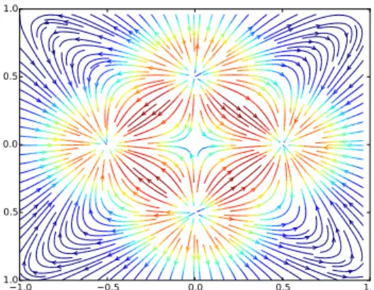
Curl-free and divergence-free kernels provide an interesting application of operator-valued kernels (Macedo and Castro, 2008; Baldassarre et al., 2012; Micheli and Glaunes, 2013) to vector field learning, for which input and output spaces have the same dimensions (𝑑 = 𝑝). Applications cover shape deformation analysis (Micheli and Glaunes, 2013) and magnetic fields approximations (Wahlstr¨om et al., 2013). These kernels discussed in (Fuselier, 2006) allow encoding input-dependent similarities between vector-fields. An illustration of a synthetic 2𝐷 curl-free and divergence free fields are given respectively in Figure 1 and Figure 2. To obain the curl-free field we took the gradient of a mixture of five two dimensional Gaussians (since the gradient of a potential is always curl-free). We generated the divergence-free field by taking the orthogonal of the curl-free field.
Proposition 10 (Curl-free and Div-free kernel (Macedo and Castro, 2008))
−1.0 −0.5 0.0 0.5 1.0 −1.0 −0.5 0.0 0.5 1.0
Figure 1: Synthetic 2𝐷 curl-free field .
−1.0 −0.5 0.0 0.5 1.0 −1.0 −0.5 0.0 0.5 1.0
Figure 2: Synthetic 2𝐷 divergence-free field .
Assume 𝒳 = (R𝑑, +) and 𝒴 = R𝑝 with 𝑑 = 𝑝. The divergence-free kernel is defined as 𝐾𝑑𝑖𝑣(𝑥, 𝑧) = 𝐾0𝑑𝑖𝑣(𝛿) = (∇∇T− Δ𝐼)𝑘0(𝛿) and the curl-free kernel as 𝐾𝑐𝑢𝑟𝑙(𝑥, 𝑧) = 𝐾0𝑐𝑢𝑟𝑙(𝛿) = −∇∇T𝑘0(𝛿), where ∇ is the gradient operator , ∇∇T is the Hessian operator and Δ is the Laplacian operator.
2.5 Shift-Invariant OVK on LCA groups
The main subjects of interest of the present paper are shift-invariant Operator-Valued Kernel. When referring to a shift-invariant OVK 𝐾 : 𝒳 × 𝒳 → ℒ(𝒴) we assume that 𝒳 is a locally compact second countable topological group with identity 𝑒.
Definition 11 (Shift-invariant OVK)
A reproducing Operator-Valued Kernel 𝐾 : 𝒳 × 𝒳 → ℒ(𝒴) is called shift-invariant if for all 𝑥, 𝑧, 𝑡 ∈ 𝒳 , 𝐾(𝑥 ⋆ 𝑡, 𝑧 ⋆ 𝑡) = 𝐾(𝑥, 𝑧).
A shift-invariant kernel can be characterized by a function of one variable 𝐾𝑒 called the signature of 𝐾. Here 𝑒 denotes the neutral element of the LCA group 𝒳 endowed with the binary group operation ⋆.
Proposition 12 (Kernel signature (Carmeli et al., 2010))
Let 𝐾 : 𝒳 × 𝒳 → ℒ(𝒴) be a reproducing kernel. The following conditions are equivalents. 1. 𝐾 is a positive-definite shift-invariant Operator-Valued Kernel.
2. There is a positive-definite function 𝐾𝑒: 𝒳 → ℒ(𝒴) such that 𝐾(𝑥, 𝑧) = 𝐾𝑒(𝑧−1⋆ 𝑥). If one of the above conditions is satisfied, then ‖𝐾(𝑥, 𝑥)‖𝒴 = ‖𝐾𝑒(𝑒)‖𝒴, ∀𝑥 ∈ 𝒳 .
We recall that if 𝐾 is a 𝒴-Mercer kernel, there is a function 𝐾𝑒 such that for all 𝑥 and 𝑧 ∈ 𝒳 , 𝐾(𝑥, 𝑧) = 𝐾𝑒(𝑥 ⋆ 𝑧−1). Then an OVK 𝐾 is 𝒴-Mercer if and only if for all 𝑦 ∈ 𝒴, 𝐾𝑒(·)𝑦 ∈ 𝒞(𝒳 ; 𝒴). In other words a 𝒴-Mercer kernel is nothing but a functions whose signature is continuous and positive definite (Carmeli et al., 2010), which fulfil the conditions required for the “operator-valued” Bochner theorem to apply. Note that if 𝐾 is a shift invariant 𝒴-Mercer kernel, then ℋ𝐾 contains continuous bounded functions (Carmeli et al., 2010).
2.6 Some applications of Operator-valued kernels
We give here a non exhaustive list of works concerning Operator-Valued Kernels. A good review of Operator-Valued Kernels has been conducted in ´Alvarez et al. (2012). For a theoretical introduction to OVKs the interested reader can refer to the papers Carmeli et al. (2006); Caponnetto et al. (2008); Carmeli et al. (2010). Generalization bounds for OVK have
been studied in Sindhwani et al. (2013); Kadri et al. (2015); Sangnier et al. (2016); Maurer (2016). Operator-valued Kernel Regression has first been studied in the context of Ridge Regression and Multi-task learning by Micchelli and Pontil (2005). Multi-task regression (Micchelli and Pontil, 2004) and structured multi-class classification (Dinuzzo et al., 2011; Minh et al., 2013b; Mroueh et al., 2012) are undoubtedly the first target applications for working in Vector Valued Reproducing Kernel Hilbert Space. Operator-Valued Kernels have been shown useful to provide a general framework for structured output prediction (Brouard et al., 2011, 2016a) with a link to Output Kernel Regression (Kadri et al., 2013).
Beyond structured classification, other various applications such as link prediction, drug activity prediction or recently metabolite identification (Brouard et al., 2016b) and image colorization (Ha Quang et al., 2010) have been developed.
Macedo and Castro (2008); Baldassarre et al. (2012) showed the interest of spectral algorithms in Ridge regression and introduced vector field learning as a new multiple output task in Machine Learning community. Wahlstr¨om et al. (2013) applied vector field learning with OVK-based Gaussian processes to the reconstruction of magnetic fields (which are curl-free). The works of Kadri et al. (2010, 2015) have been the precursors of regression with functional values, opening a new avenue of applications. Appropriate algorithms devoted to online learning have been also derived by Audiffren and Kadri (2015). Kernel learning was addressed at least in two ways: first with using Multiple Kernel Learning in Kadri et al. (2012) and second, using various penalties, smooth ones in Dinuzzo et al. (2011); Ciliberto et al. (2015) for decomposable kernels and non smooth ones in Lim et al. (2015b) using proximal methods in the case of decomposable and transformable kernels. Dynamical modeling was tackled in the context of multivariate time series modelling in Lim et al. (2013); Sindhwani et al. (2013); Lim et al. (2015b) and as a generalization of Recursive Least
Square Algorithm in Amblard and Kadri (2015). Sangnier et al. (2016) recently explored the minimization of a pinball loss under regularizing constraints induced by a well chosen decomposable kernel in order to handle joint quantile regression.
3. Main contribution: Operator Random Fourier Features
We present in this section a construction methodology devoted to shift-invariant 𝒴-Mercer operator-valued kernels defined on any Locally Compact Abelian (LCA) group, noted (𝒳 , ⋆), for some operation noted ⋆. This allows us to use the general context of Pontryagin duality for Fourier Transform of functions on LCA groups. Building upon a generalization of the celebrated Bochner’s theorem for operator-valued measures, an operator-valued kernel is seen as the Fourier Transform of an operator-valued positive measure. From that result, we extend the principle of RFF for scalar-valued kernels and derive a general methodology to build Operator-valued Random Fourier Feature (ORFF) when operator-valued kernels are
shift-invariant according to the chosen group operation. Elements of this paper have been developped in Brault et al. (2016).
We present a construction of feature maps called Operator-valued Random Fourier Feature (ORFF), such that 𝑓 : 𝑥 ↦→ ̃︀𝜑(𝑥)*𝜃 is a continuous function that maps an arbitrary LCA group 𝒳 as input space to an arbitrary output Hilbert space 𝒴. First we define a functional Fourier feature map, and then propose a Monte-Carlo sampling from this feature map to construct an approximation of a shift-invariant 𝒴-Mercer kernel. Then, we prove the convergence of the kernel approximation ˜𝐾(𝑥, 𝑧) = ̃︀𝜑(𝑥)*𝜑(𝑧) with high probability oñ︀ compact subsets of the LCA 𝒳 . Eventually we conclude with some numerical experiments. 3.1 Theoretical study
The following proposition of Zhang et al. (2012); Neeb (1998) extends Bochner’s theorem to any shift-invariant 𝒴-Mercer kernel. We give a short intoduction to LCA groups and abstract harmonic analysis in appendix A. For the sake of simplicity, the reader can take (𝑥, 𝜔) = exp(i⟨𝑥, 𝜔⟩2) = exp(−i⟨𝑥, 𝜔⟩2), when 𝑥 ∈ 𝒳 = (R𝑑, +).
Proposition 13 (Operator-valued Bochner’s theorem (Zhang et al., 2012; Neeb, 1998)) If a function 𝐾 from 𝒳 × 𝒳 to 𝒴 is a shift-invariant 𝒴-Mercer kernel on 𝒳 , then there exists a unique positive projection-valued measure ̂︀𝑄 : ℬ(𝒳 ) → ℒ+(𝒴) such that for all 𝑥, 𝑧 ∈ 𝒳 , (6 ) 𝐾(𝑥, 𝑧) = ∫︁ ̂︀ 𝒳 (𝑥 ⋆ 𝑧−1, 𝜔)𝑑 ̂︀𝑄(𝜔),
where ̂︀𝑄 belongs to the set of all the projection-valued measures of bounded variation on the 𝜎-algebra of Borel subsets of ̂︀𝒳 . Conversely, from any positive operator-valued measure ̂︀𝑄, a shift-invariant kernel 𝐾 can be defined by Equation 6.
Although this theorem is central to the spectral decomposition of shift-invariant 𝒴-Mercer OVK, the following results proved by Carmeli et al. (2010) provides insights about this decomposition that are more relevant in practice. It first gives the necessary conditions to build shift-invariant 𝒴-Mercer kernel with a pair (𝐴,𝜇) where 𝐴 is an operator-valued̂︀ function on ̂︀𝒳 and𝜇 is a real-valued positive measure on ̂︀̂︀ 𝒳 . Note that obviously such a pair is not unique and the choice of this paper may have an impact on theoretical properties as well as practical computations. Secondly it also states that any OVK have such a spectral decomposition when 𝒴 is finite dimensional or 𝒳 .
Proposition 14 (Carmeli et al. (2010))
Let ̂︀𝜇 be a positive measure on ℬ( ̂︀𝒳 ) and 𝐴 : ̂︀𝒳 → ℒ(𝒴) such that ⟨𝐴(·)𝑦, 𝑦′⟩ ∈ 𝐿1(𝒳 , ̂︀ 𝜇) for all 𝑦, 𝑦′∈ 𝒴 and 𝐴(𝜔) < 0 for ̂︀𝜇-almost all 𝜔 ∈ ̂︀𝒳 . Then, for all 𝛿 ∈ 𝒳 ,
(7 ) 𝐾𝑒(𝛿) = ∫︁ ̂︀ 𝒳 (𝛿, 𝜔)𝐴(𝜔)𝑑𝜇(𝜔)̂︀
is the kernel signature of a shift-invariant 𝒴-Mercer kernel 𝐾 such that 𝐾(𝑥, 𝑧) = 𝐾𝑒(𝑥⋆𝑧−1). The VV-RKHS ℋ𝐾 is embed in 𝐿2( ̂︀𝒳 ,𝜇; 𝒴̂︀
′) by means of the feature operator
(8 ) (𝑊 𝑔)(𝑥) = ∫︁ ̂︀ 𝒳 (𝑥, 𝜔)𝐵(𝜔)𝑔(𝜔)𝑑𝜇(𝜔),̂︀
Where 𝐵(𝜔)𝐵(𝜔)* = 𝐴(𝜔) and both integrals converge in the weak sense. If 𝒴 is finite dimensional or 𝒳 is compact, any shift-invariant kernel is of the above form for some pair (𝐴,𝜇).̂︀
When 𝑝 = 1 one can always assume 𝐴 is reduced to the scalar 1, 𝜇 is still a bounded̂︀ positive measure and we retrieve the Bochner theorem applied to the scalar case (Theorem 1).
Proposition 14 shows that a pair (𝐴,̂︀𝜇) entirely characterizes an OVK. Namely a given measure𝜇 and a function 𝐴 such that ⟨𝑦̂︀ ′, 𝐴(𝑐˙)𝑦⟩𝒴 ∈ 𝐿1(𝒳 ,
̂︀
𝜇) for all 𝑦, 𝑦′ ∈ 𝒴 and 𝐴(𝜔) < 0 for𝜇-almost all 𝜔, give rise to an OVK. Since (𝐴,̂︀ ̂︀𝜇) determine a unique kernel we can write ℋ(𝐴,
̂︀
𝜇) =⇒ℋ𝐾 where 𝐾 is defined as in Equation 7. However the converse is not true: Given a 𝒴-Mercer shift invariant Operator-Valued Kernel, there exist infinitely many pairs (𝐴,𝜇)̂︀ that characterize an OVK.
The main difference between Equation 6 and Equation 7 is that the first one characterizes an OVK by a unique Positive Operator-Valued Measure (POVM), while the second one shows that the POVM that uniquely characterizes a 𝒴-Mercer OVK has an operator-valued density with respect to a scalar measure 𝜇; and that this operator-valued density is not̂︀ unique. Notice that obtaining a scalar-valued density from the POVM implies the addition of a (weak) 𝐿1 condition on 𝐾𝑒.
Finally Proposition 14 does not provide any constructive way to obtain the pair (𝐴,̂︀𝜇) that characterizes an OVK. The following Subsection 3.1.1 is based on another proposition of Carmeli et al. and shows that if the kernel signature 𝐾𝑒(𝛿) of an OVK is in 𝐿1 then it is possible to construct explicitly a pair (𝐶, \Haar) from it. Additionally, we show that we can always extract a scalar-valued probability density function from 𝐶 such that we obtain a pair (𝐴, Pr̂︀𝜇,𝜌) where Pr𝜇,𝜌̂︀ is a probability distribution absolutely continuous with respect to 𝜇 and with associated probibility density function (p. d. f) 𝜌. Thus for̂︀ all 𝒵 ⊂ ℬ( ̂︀𝒳 ), Pr
̂︀
𝜇,𝜌(𝒵) = ∫︀
𝒵𝜌(𝜔)𝑑𝜇(𝜔). When the reference measurê︀ ̂︀𝜇 is the Lebesgue measure, we note Pr
̂︀
𝜇,𝜌 = Pr𝜌. For any function 𝑓 : 𝒳 × ̂︀𝒳 × 𝒴 → R, we also use the notation EHaar,𝜌\ [𝑓 (𝑥, 𝜔, 𝑦)] = E𝜔∼Pr
\ Haar,𝜌[𝑓 (𝑥, 𝜔, 𝑦)] = ∫︀ ̂︀ 𝒳𝑓 (𝑥, 𝜔, 𝑦)𝑑PrHaar,𝜌\ (𝜔) = ∫︀ ̂︀
𝒳𝑓 (𝑥, 𝜔, 𝑦)𝜌(𝜔)𝑑\Haar(𝜔). where the two last equalities hold by the “law of the unconscious statistician” (change of variable formula) and the fact that PrHaar,𝜌\ has density 𝜌. Hence depending on the context, with mild abuse of notation, we view 𝜔 either as a variable in the probability space ( ̂︀𝒳 , Pr
\
Haar,𝜌) or as a random variable with values in ̂︀𝒳 and distributed as PrHaar,𝜌\ .
3.1.1 Sufficient conditions of existence
While Proposition 14 gives some insights on how to build an approximation of a 𝒴-Mercer kernel, we need a theorem that provides an explicit construction of the pair (𝐴, Pr
̂︀
𝜇,𝜌) from the kernel signature 𝐾𝑒. Proposition 14 in Carmeli et al. (2010) gives the solution, and also provides a sufficient condition for Proposition 14 to apply.
Proposition 15 (Carmeli et al. (2010))
Let 𝐾 be a shift-invariant 𝒴-Mercer kernel of signature 𝐾𝑒. Suppose that for all 𝑧 ∈ 𝒳 and for all 𝑦, 𝑦′ ∈ 𝒴, the function ⟨𝐾𝑒(.)𝑦, 𝑦′⟩𝒴 ∈ 𝐿1(𝒳 , Haar) where 𝒳 is endowed with the
group law ⋆. Denote 𝐶 : ̂︀𝑋 → ℒ(𝑌 ), the function defined for all 𝜔 ∈ ̂︀𝒳 that satisfies for all 𝑦, 𝑦′ in 𝒴: (9 ) ⟨𝑦′, 𝐶(𝜔)𝑦⟩𝒴 = ∫︁ 𝒳 (𝛿, 𝜔)⟨𝑦′, 𝐾𝑒(𝛿)𝑦⟩𝒴𝑑Haar(𝛿) = ℱ −1[︀⟨𝑦′ , 𝐾𝑒(·)𝑦⟩𝒴]︀ (𝜔). Then
1. 𝐶(𝜔) is a bounded non-negative operator for all 𝜔 ∈ ̂︀𝒳 , 2. ⟨𝑦, 𝐶(·)𝑦′⟩𝒴 ∈ 𝐿1(︁
̂︀
𝒳 , \Haar)︁ for all 𝑦, 𝑦′ ∈ 𝒳 , 3. for all 𝛿 ∈ 𝒳 and for all 𝑦, 𝑦′ in 𝒴, ⟨𝑦′, 𝐾𝑒(𝛿)𝑦⟩𝒴 =
∫︀ ̂︀ 𝒳 (𝛿, 𝜔)⟨𝑦 ′, 𝐶(𝜔)𝑦⟩ 𝒴𝑑\Haar(𝜔) = ℱ[︀⟨𝑦′, 𝐶(·)𝑦⟩ 𝒴]︀ (𝛿).
We found some confusion in the literature whether a kernel is the Fourier Transform or Inverse Fourier Transform of a measure. However Lemma 16 clarifies the relation between the Fourier Transform and Inverse Fourier Transform for a translation invariant Operator-Valued Kernel. Notice that in the real scalar case the Fourier Transform and Inverse Fourier Transform of a shift-invariant kernel are the same, while the difference is significant for OVK. The following lemma is a direct consequence of the definition of 𝐶(𝜔) as the Fourier Transform of the adjoint of 𝐾𝑒 and also helps to simplify the definition of ORFF.
Lemma 16
Let 𝐾𝑒 be the signature of a shift-invariant 𝒴-Mercer kernel such that for all 𝑦, 𝑦′ ∈ 𝒴, ⟨𝑦′, 𝐾𝑒(·)𝑦⟩𝒴 ∈ 𝐿1(𝒳 , Haar) and let ⟨𝑦′, 𝐶(·)𝑦⟩𝒴 = ℱ−1[︀⟨𝑦′, 𝐾𝑒(·)𝑦⟩𝒴]︀. Then
1. 𝐶(𝜔) is self-adjoint and 𝐶 is even. 2. ℱ−1[︀⟨𝑦′, 𝐾𝑒(·)𝑦⟩𝒴]︀ = ℱ [︀⟨𝑦′, 𝐾𝑒(·)𝑦⟩𝒴]︀. 3. 𝐾𝑒(𝛿) is self-adjoint and 𝐾𝑒 is even.
While Proposition 15 gives an explicit form of the operator 𝐶(𝜔) defined as the Fourier Transform of the kernel 𝐾, it is not really convenient to work with the Haar measure \Haar on ℬ( ̂︀𝒳 ). However it is easily possible to turn \Haar into a probability measure to allow efficient integration over an infinite domain.
The following proposition allows to build a spectral decomposition of a shift-invariant 𝒴-Mercer kernel on a LCA group 𝒳 endowed with the group law ⋆ with respect to a scalar probability measure, by extracting a scalar probability density function from 𝐶.
Proposition 17 (Shift-invariant 𝒴-Mercer kernel spectral decomposition)
Let 𝐾𝑒be the signature of a shift-invariant 𝒴-Mercer kernel. If for all 𝑦, 𝑦′∈ 𝒴, ⟨𝐾𝑒(.)𝑦, 𝑦′⟩ ∈ 𝐿1(𝒳 , Haar) then there exists a positive probability measure PrHaar,𝜌\ and an operator-valued function 𝐴 an such that for all 𝑦, 𝑦′ ∈ 𝒴,
(10 ) ⟨𝑦′, 𝐾𝑒(𝛿)𝑦⟩𝒴 = EHaar,𝜌\ [︁ (𝛿, 𝜔)⟨𝑦′, 𝐴(𝜔)𝑦⟩𝒴 ]︁ , with ⟨𝑦′, 𝐴(𝜔)𝑦⟩𝒴𝜌(𝜔) = ℱ [⟨𝑦′, 𝐾𝑒(·)𝑦⟩]𝒴(𝜔). Moreover
1. for all 𝑦, 𝑦′ ∈ 𝒴, ⟨𝐴(·)𝑦, 𝑦′⟩
𝒴 ∈ 𝐿1( ̂︀𝒳 , PrHaar,𝜌\ ), 2. 𝐴(𝜔) is non-negative for PrHaar,𝜌\ -almost all 𝜔 ∈ ̂︀𝒳 , 3. 𝐴(·) and 𝜌(·) are even functions.
3.2 Examples of spectral decomposition
In this section we give examples of spectral decomposition for various 𝒴-Mercer kernels, based on Proposition 17.
3.2.1 Gaussian decomposable kernel
Recall that a decomposable R𝑝-Mercer introduced in Proposition 8 has the form 𝐾(𝑥, 𝑧) = 𝑘(𝑥, 𝑧)Γ, where 𝑘(𝑥, 𝑧) is a scalar Mercer kernel and Γ ∈ ℒ(R𝑝) is a non-negative operator. Let us focus on 𝐾𝑒𝑑𝑒𝑐,𝑔𝑎𝑢𝑠𝑠(·) = 𝑘𝑔𝑎𝑢𝑠𝑠𝑒 (·)Γ, the Gaussian decomposable kernel where 𝐾𝑒𝑑𝑒𝑐,𝑔𝑎𝑢𝑠𝑠 and 𝑘𝑔𝑎𝑢𝑠𝑠𝑒 are respectively the signature of 𝐾 and 𝑘 on the additive group 𝒳 = (R𝑑, +) – 𝑖. 𝑒. 𝛿 = 𝑥 − 𝑧 and 𝑒 = 0. The well known Gaussian kernel is defined for all 𝛿 ∈ R𝑑as follows 𝑘gauss0 (𝛿) = exp
(︁
−𝜎−2‖𝛿‖22)︁/2 where 𝜎 ∈ R>0 is an hyperparameter corresponding to the bandwith of the kernel. The –Pontryagin– dual group of 𝒳 = (R𝑑, +) is ̂︀𝒳 ∼= (R𝑑, +) with the pairing (𝛿, 𝜔) = exp (i⟨𝛿, 𝜔⟩2) where 𝛿 and 𝜔 ∈ R𝑑. In this case the Haar measures on 𝒳 and ̂︀𝒳 are in both cases the Lebesgue measure. However in order to have the property that ℱ−1[ℱ [𝑓 ]] = 𝑓 and ℱ−1[𝑓 ] = ℛℱ [𝑓 ] one must normalize both measures by√2𝜋−𝑑, i. e. for all 𝒵 ∈ ℬ(︀
R𝑑)︀, √
2𝜋𝑑Haar(𝒵) = Leb(𝒵) and√2𝜋𝑑Haar(𝒵) = Leb(𝒵). Then the Fourier\ Transform on (R𝑑, +) is
ℱ [𝑓 ] (𝜔) = ∫︁
R𝑑
exp (−i⟨𝛿, 𝜔⟩2) 𝑓 (𝛿)𝑑Haar(𝛿) = ∫︁
R𝑑
exp (−i⟨𝛿, 𝜔⟩2) 𝑓 (𝛿)𝑑Leb(𝛿)√ 2𝜋𝑑
. Since 𝑘0gauss∈ 𝐿1 and Γ is bounded, it is possible to apply Proposition 17, and obtain for all 𝑦 and 𝑦′ ∈ 𝒴, ⟨ 𝑦′, 𝐶𝑑𝑒𝑐,𝑔𝑎𝑢𝑠𝑠(𝜔)𝑦 ⟩ 2 = ℱ [︁⟨ 𝑦′, 𝐾0𝑑𝑒𝑐,𝑔𝑎𝑢𝑠𝑠(·)𝑦 ⟩ 2 ]︁ (𝜔) = ℱ [𝑘𝑔𝑎𝑢𝑠𝑠0 ] (𝜔)⟨︀𝑦′, Γ𝑦⟩︀2. Thus 𝐶𝑑𝑒𝑐,𝑔𝑎𝑢𝑠𝑠(𝜔) = ∫︁ R𝑑 exp (︃ −i⟨𝜔, 𝛿⟩2−‖𝛿‖ 2 2 2𝜎2 )︃ 𝑑Leb(𝛿) √ 2𝜋𝑑 Γ. Hence 𝐶𝑑𝑒𝑐,𝑔𝑎𝑢𝑠𝑠(𝜔) = 1 √︁ 2𝜋𝜎12 𝑑exp (︂ −𝜎 2 2 ‖𝜔‖ 2 2 )︂√ 2𝜋𝑑 ⏟ ⏞ 𝜌(·)=𝒩 (0,𝜎−2𝐼 𝑑) √ 2𝜋𝑑 Γ ⏟ ⏞ 𝐴(·)=Γ .
Therefore the canonical decomposition of 𝐶𝑑𝑒𝑐,𝑔𝑎𝑢𝑠𝑠 is 𝐴𝑑𝑒𝑐,𝑔𝑎𝑢𝑠𝑠(𝜔) = Γ and 𝜌𝑑𝑒𝑐,𝑔𝑎𝑢𝑠𝑠 = 𝒩 (0, 𝜎−2𝐼
𝑑) √
2𝜋𝑑, where 𝒩 is the Gaussian probability distribution. Note that this decom-position is done with respect to the normalized Lebesgue measure \Haar, meaning that for
all 𝒵 ∈ ℬ( ̂︀𝒳 ), Pr \ Haar,𝒩 (0,𝜎−2𝐼 𝑑) √ 2𝜋𝑑(𝒵) = ∫︁ 𝒵 𝒩 (0, 𝜎−2𝐼𝑑) √ 2𝜋𝑑𝑑\Haar(𝜔) = ∫︁ ̂︀ 𝒳 𝒩 (0, 𝜎−2𝐼𝑑)𝑑Leb(𝜔) = Pr𝒩 (0,𝜎−2𝐼 𝑑)(𝒵).
Thus, the same decomposition with respect to the usual –non-normalized– Lebesgue measure Leb yields
(11a) 𝐴𝑑𝑒𝑐,𝑔𝑎𝑢𝑠𝑠(·) = Γ
(11b) 𝜌𝑑𝑒𝑐,𝑔𝑎𝑢𝑠𝑠= 𝒩 (0, 𝜎−2𝐼𝑑).
3.2.2 Skewed-𝜒2 decomposable kernel
The skewed-𝜒2 scalar kernel (Li et al., 2010), useful for image processing, is defined on the LCA group 𝒳 = (−𝑐𝑘; +∞)𝑑𝑘=1, with 𝑐𝑘 ∈ R>0 and endowed with the group operation ⊙. Let (𝑒𝑘)𝑑𝑘=1 be the standard basis of 𝒳 . The operator ⊙ : 𝒳 × 𝒳 → 𝒳 is defined by 𝑥 ⊙ 𝑧 = ((𝑥𝑘+ 𝑐𝑘)(𝑧𝑘+ 𝑐𝑘) − 𝑐𝑘)𝑑𝑘=1. The identity element 𝑒 is (1 − 𝑐𝑘)𝑑𝑘=1 since (1 − 𝑐) ⊙ 𝑥 = 𝑥. Thus the inverse element 𝑥−1 is ((𝑥𝑘+ 𝑐𝑘)−1− 𝑐𝑘)𝑑𝑘=1. The skewed-𝜒2 scalar kernel reads
(12) 𝑘𝑠𝑘𝑒𝑤𝑒𝑑1−𝑐 (𝛿) = 𝑑 ∏︁ 𝑘=1 2 √ 𝛿𝑘+ 𝑐𝑘+ √︁ 1 𝛿𝑘+𝑐𝑘 .
The dual of 𝒳 is ̂︀𝒳 ∼= R𝑑 with the pairing (𝛿, 𝜔) =∏︀𝑑
𝑘=1exp (i log(𝛿𝑘+ 𝑐𝑘)𝜔𝑘). The Haar measure are defined for all 𝒵 ∈ ℬ((−𝑐; +∞)𝑑) and all ̂︀𝒵 ∈ ℬ(R𝑑) by √2𝜋𝑑Haar(𝒵) = ∫︀
𝒵 ∏︀𝑑
𝑘=1𝑧𝑘+𝑐1 𝑘𝑑Leb(𝑧) and √
2𝜋𝑑Haar( ̂︀\ 𝒵) = Leb( ̂︀𝒵). Thus the Fourier Transform is
ℱ [𝑓 ] (𝜔) = ∫︁ (−𝑐;+∞)𝑑 𝑑 ∏︁ 𝑘=1
exp (−i log(𝛿𝑘+ 𝑐𝑘)𝜔𝑘) 𝛿𝑘+ 𝑐𝑘
𝑓 (𝛿)𝑑Leb(𝛿)√ 2𝜋𝑑
.
Then, applying Fubini’s theorem over product space, and the fact that each dimension is independent ℱ[︁𝑘0𝑠𝑘𝑒𝑤𝑒𝑑]︁(𝜔) = 𝑑 ∏︁ 𝑘=1 ∫︁ +∞ −𝑐𝑘
2 exp (−i log(𝛿𝑘+ 𝑐𝑘)𝜔𝑘) (𝛿𝑘+ 𝑐𝑘) (︁√ 𝛿𝑘+ 𝑐𝑘+ √︁ 1 𝛿𝑘+𝑐𝑘 )︁ 𝑑Leb(𝛿𝑘) √ 2𝜋𝑑 .
Making the change of variable 𝑡𝑘 = (𝛿𝑘+ 𝑐𝑘)−1 yields ℱ[︁𝑘𝑠𝑘𝑒𝑤𝑒𝑑0 ]︁(𝜔) = 𝑑 ∏︁ 𝑘=1 ∫︁ +∞ −∞ 2 exp (−i𝑡𝑘𝜔𝑘) exp(︀1 2𝑡𝑘)︀ + exp (︀− 1 2𝑡𝑘 )︀ 𝑑Leb(𝑡𝑘) √ 2𝜋𝑑 =√2𝜋𝑑 𝑑 ∏︁ 𝑘=1 sech(𝜋𝜔𝑘).
Since 𝑘1−𝑐skewed∈ 𝐿1 and Γ is bounded, it is possible to apply Proposition 17, and obtain
𝐶𝑑𝑒𝑐,𝑠𝑘𝑒𝑤𝑒𝑑(𝜔) = ℱ[︁𝑘1−𝑐𝑠𝑘𝑒𝑤𝑒𝑑]︁(𝜔)Γ =√2𝜋𝑑 𝑑 ∏︁ 𝑘=1 sech(𝜋𝜔𝑘) ⏟ ⏞ 𝜌(·)=𝒮(0,2−1)𝑑√2𝜋𝑑 Γ ⏟ ⏞ 𝐴(·) .
Hence the decomposition with respect to the usual –non-normalized– Lebesgue measure Leb yields (13a) 𝐴𝑑𝑒𝑐,𝑠𝑘𝑒𝑤𝑒𝑑(·) = Γ (13b) 𝜌𝑑𝑒𝑐,𝑠𝑘𝑒𝑤𝑒𝑑 = 𝒮(︀0, 2−1)︀𝑑.
3.2.3 Curl-free Gaussian kernel
The curl-free Gaussian kernel is defined as 𝐾0𝑐𝑢𝑟𝑙,𝑔𝑎𝑢𝑠𝑠= −∇∇T𝑘𝑔𝑎𝑢𝑠𝑠0 . Here 𝒳 = (R𝑑, +) so the setting is the same than Subsection 3.2.1.
𝐶𝑐𝑢𝑟𝑙,𝑔𝑎𝑢𝑠𝑠(𝜔)𝑖𝑗 = ℱ [︁ 𝐾1−𝑐𝑐𝑢𝑟𝑙,𝑔𝑎𝑢𝑠𝑠(·)𝑖𝑗 ]︁ (𝜔) = √︂ 2𝜋 1 𝜎2 𝑑 exp (︂ −𝜎 2 2 ‖𝜔‖ 2 2 )︂√ 2𝜋𝑑𝜔𝑖𝜔𝑗. Hence 𝐶𝑐𝑢𝑟𝑙,𝑔𝑎𝑢𝑠𝑠(𝜔) = 1 √︁ 2𝜋𝜎12 𝑑exp (︂ −𝜎 2 2 ‖𝜔‖ 2 2 )︂√ 2𝜋𝑑 ⏟ ⏞ 𝜇(·)=𝒩 (0,𝜎−2𝐼 𝑑) √ 2𝜋𝑑 𝜔𝜔T ⏟ ⏞ 𝐴(𝜔)=𝜔𝜔T .
Here a canonical decomposition is 𝐴𝑐𝑢𝑟𝑙,𝑔𝑎𝑢𝑠𝑠(𝜔) = 𝜔𝜔T for all 𝜔 ∈ R𝑑 and 𝜇𝑐𝑢𝑟𝑙,𝑔𝑎𝑢𝑠𝑠 = 𝒩 (0, 𝜎−2𝐼
𝑑) √
2𝜋𝑑 with respect to the normalized Lebesgue measure 𝑑𝜔. Again the decom-position with respect to the usual –non-normalized– Lebesgue measure is for all 𝜔 ∈ R𝑑
(14a) 𝐴𝑐𝑢𝑟𝑙,𝑔𝑎𝑢𝑠𝑠(𝜔) = 𝜔𝜔T
(14b) 𝜇𝑐𝑢𝑟𝑙,𝑔𝑎𝑢𝑠𝑠= 𝒩 (0, 𝜎−2𝐼𝑑).
3.2.4 Divergence-free kernel
The divergence-free Gaussian kernel is defined as 𝐾0𝑑𝑖𝑣,𝑔𝑎𝑢𝑠𝑠= (∇∇T− Δ)𝑘0𝑔𝑎𝑢𝑠𝑠on the group 𝒳 = (R𝑑, +). The setting is the same than Subsection 3.2.1. Hence
𝐶𝑑𝑖𝑣,𝑔𝑎𝑢𝑠𝑠(𝜔)𝑖𝑗 = ℱ [︁ 𝐾0𝑑𝑖𝑣,𝑔𝑎𝑢𝑠𝑠(·)𝑖𝑗 ]︁ (𝜔) = (︃ 𝛿𝑖=𝑗 𝑑 ∑︁ 𝑘=1 𝜔2𝑘− 𝜔𝑖𝜔𝑗 )︃ ℱ [𝑘0𝑔𝑎𝑢𝑠𝑠] (𝜔). Hence 𝐶𝑑𝑖𝑣,𝑔𝑎𝑢𝑠𝑠(𝜔) = 1 √︁ 2𝜋𝜎12 𝑑exp (︂ −𝜎 2 2 ‖𝜔‖ 2 2 )︂√ 2𝜋𝑑 ⏟ ⏞ 𝜌(·)=𝒩 (0,𝜎−2𝐼 𝑑) √ 2𝜋𝑑 (︁ 𝐼𝑑‖𝜔‖22− 𝜔𝜔T )︁ ⏟ ⏞ 𝐴(𝜔)=𝐼𝑑‖𝜔‖22−𝜔𝜔T .
Thus the canonical decomposition with respect to the normalized Lebesgue measure is 𝐴𝑑𝑖𝑣,𝑔𝑎𝑢𝑠𝑠(𝜔) = 𝐼𝑑‖𝜔‖22− 𝜔𝜔T and the measure 𝜌𝑑𝑖𝑣,𝑔𝑎𝑢𝑠𝑠 = 𝒩 (0, 𝜎−2𝐼𝑑)
√
2𝜋𝑑. The canonical decomposition with respect to the usual Lebesgue measure is
(15a) 𝐴𝑑𝑖𝑣,𝑔𝑎𝑢𝑠𝑠(𝜔) = 𝐼𝑑‖𝜔‖22− 𝜔𝜔T
(15b) 𝜌𝑑𝑖𝑣,𝑔𝑎𝑢𝑠𝑠= 𝒩 (0, 𝜎−2𝐼𝑑).
3.3 Operator-valued Random Fourier Features (ORFF) 3.3.1 Building Operator-valued Random Fourier Features
As shown in Proposition 17 it is always possible to find a pair (𝐴, PrHaar,𝜌\ ) from a shift invariant 𝒴-Mercer Operator-Valued Kernel 𝐾𝑒 such that PrHaar,𝜌\ is a probability measure, i. e. ∫︀
̂︀
𝒳𝜌𝑑\Haar = 1 where 𝜌 is the density of PrHaar,𝜌\ and 𝐾𝑒(𝛿) = EHaar,𝜌\ (𝛿, 𝜔)𝐴(𝜔). In order to obtain an approximation of 𝐾 from a decomposition (𝐴, PrHaar,𝜌\ ) we turn our attention to a Monte-Carlo estimation of the expectation in Equation 10 characterizing a 𝒴-Mercer shift-invariant Operator-Valued Kernel.
Proposition 18
Let 𝐾(𝑥, 𝑧) be a shift-invariant 𝒴-Mercer kernel with signature 𝐾𝑒 such that for all 𝑦, 𝑦′∈ 𝒴, ⟨𝑦′, 𝐾𝑒(·)𝑦⟩𝒴 ∈ 𝐿1(𝒳 , Haar). Then one can find a pair (𝐴, PrHaar,𝜌\ ) that satisfies Proposition 17. i. e. for PrHaar,𝜌\ -almost all 𝜔, and all 𝑦, 𝑦′ ∈ 𝒴, ⟨𝑦, 𝐴(𝜔)𝑦′⟩𝜌(𝜔) = ℱ [⟨𝑦′, 𝐾𝑒(·)𝑦⟩] (𝜔). If (𝜔𝑗)𝐷𝑗=1 be a sequence of 𝐷 ∈ N
* i. i. d. random variables following the law Pr
\
Haar,𝜌 then the operator-valued function ˜𝐾 defined for (𝑥, 𝑧) ∈ 𝒳 × 𝒳 as
˜ 𝐾(𝑥, 𝑧) = 1 𝐷 𝐷 ∑︁ 𝑗=1 (𝑥 ⋆ 𝑧−1, 𝜔 𝑗)𝐴(𝜔𝑗)
is an approximation of 𝐾. i. e. it satisfies for all 𝑥, 𝑧 ∈ 𝒳 , ˜𝐾(𝑥, 𝑧)−−−−→a. s.
𝐷→∞ 𝐾(𝑥, 𝑧) in the weak operator topology, where 𝐾 is a 𝒴-Mercer OVK.
Now, for efficient computations as motivated in the introduction, we are interested in finding an approximated feature map instead of a kernel approximation. Indeed, an approximated feature map will allow to build linear models in regression tasks. The following proposition deals with the feature map construction.
Proposition 19
Assume the same conditions as Proposition 18. Moreover, if one can define 𝐵 : ̂︀𝒳 → ℒ(𝒴′, 𝒴) such that for PrHaar,𝜌\ -almost all 𝜔, and all 𝑦, 𝑦′ ∈ 𝒴, ⟨𝑦, 𝐵(𝜔)𝐵(𝜔)*𝑦′⟩𝒴𝜌(𝜔) = ⟨𝑦, 𝐴(𝜔)𝑦′⟩𝜌(𝜔) = ℱ[︀⟨𝑦, 𝐾𝑒(·)𝑦′⟩𝒴]︀ (𝜔), then the function 𝜑 : ̂︀̃︀ 𝒳 → ℒ(𝒴,
⨁︀𝐷 𝑗=1𝒴
′) defined for all 𝑦 ∈ 𝒴 as follows:
̃︀ 𝜑(𝑥)𝑦 = √1 𝐷 𝐷 ⨁︁ 𝑗=1 (𝑥, 𝜔𝑗)𝐵(𝜔𝑗)*𝑦, 𝜔𝑗 ∼ PrHaar,𝜌\ i. i. d.,
is an approximated feature map2 for the kernel 𝐾. Remark 20
2. i. e. it satisfies for all 𝑥, 𝑧 ∈ 𝒳 , ̃︀𝜑(𝑥)*𝜑(𝑧)̃︀ a. s. −−−−→
𝐷→∞ 𝐾(𝑥, 𝑧) in the weak operator topology, where 𝐾 is a
Algorithm 1: Construction of ORFF from OVK
Input : 𝐾(𝑥, 𝑧) = 𝐾𝑒(𝛿) a shift-invariant 𝒴-Mercer kernel on (𝒳 , ⋆) such that ∀𝑦, 𝑦′ ∈ 𝒴, ⟨𝑦′, 𝐾𝑒(·)𝑦⟩𝒴 ∈ 𝐿1(R𝑑, Haar) and 𝐷 the number of features. Output : A random feature ̃︀𝜑(𝑥) such that ̃︀𝜑(𝑥)*𝜑(𝑧) ≈ 𝐾(𝑥, 𝑧)̃︀
1 Define the pairing (𝑥, 𝜔) from the LCA group (𝒳 , ⋆); 2 Find a decomposition (𝐴, Pr
\
Haar,𝜌) and 𝐵 such that
𝐵(𝜔)𝐵(𝜔)*𝜌(𝜔) = 𝐴(𝜔)𝜌(𝜔) = ℱ−1[𝐾𝑒] (𝜔); 4
4 Draw 𝐷 i. i. d. realizations (𝜔𝑗)𝐷𝑗=1 from the probability distribution PrHaar,𝜌\ ;
6 6 return ⎧ ⎨ ⎩ ̃︀ 𝜑(𝑥) ∈ ℒ(𝒴, ̃︀ℋ) : 𝑦 ↦→ √1 𝐷 ⨁︀𝐷 𝑗=1(𝑥, 𝜔𝑗)𝐵(𝜔𝑗) *𝑦 ̃︀ 𝜑(𝑥)*∈ ℒ( ̃︀ℋ, 𝒴) : 𝜃 ↦→ √1 𝐷 ∑︀𝐷 𝑗=1(𝑥, 𝜔𝑗)𝐵(𝜔𝑗)𝜃𝑗 ;
We find a decomposition such that 𝐴(𝜔𝑗) = 𝐵(𝜔𝑗)𝐵(𝜔𝑗)* for all 𝑗 ∈ N*𝐷 either by exhibiting a closed-form or using a numerical decomposition. Such a decomposition always exists since 𝐴(𝜔) is positive semi-definite for all 𝜔 ∈ ̂︀𝒳 .
Notice that an ORFF map as defined in Proposition 19 is also the Monte-Carlo sampling of the corresponding functional Fourier feature map 𝜑𝑥 : 𝒴 → 𝐿2( ̂︀𝒳 , PrHaar,𝜌\ ; 𝒴′) as defined in Proposition 21. Indeed, for all 𝑦 ∈ 𝒴 and all 𝑥 ∈ 𝒳 , ̃︀𝜑(𝑥)𝑦 = ⨁︀𝐷
𝑗=1(𝜑𝑥𝑦)(𝜔𝑗), 𝜔𝑗 ∼ PrHaar,𝜌\ i. i. d. Proposition 19 allows us to define Algorithm 1 for constructing ORFF from an operator valued kernel.
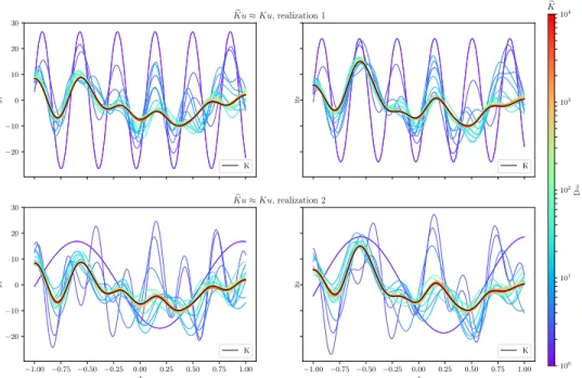
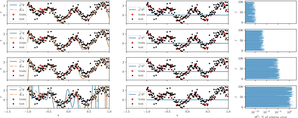
We give a numerical illustration of different ˜𝐾 built from different i. i. d. realization (𝜔𝑗)𝐷𝑗=1, 𝜔𝑗 ∼ PrHaar,𝜌\ . In Figure 3, we represent the approximation of a reference function (black line) defined as (𝑦1, 𝑦2)T= 𝑓 (𝑥𝑖) =∑︀250𝑗=1K𝑖𝑗𝑢𝑗 where 𝑢𝑗 ∼ 𝒩 (0, 𝐼2) and 𝐾 is a Gaussian decomposable kernel. We took Γ = .5𝐼2+ .512 such that the outputs 𝑦1 and 𝑦2 share some similarities. We generated 250 points equally separated on the segment (−1; 1). The Gram matrix is then K𝑖𝑗 = exp
(︁
−(𝑥𝑖−𝑥𝑗)2 2(0.1)2
)︁
Γ, for 𝑖, 𝑗 ∈ N*250. We took Γ = .5𝐼2+ .512 such that the outputs 𝑦1 and 𝑦2 share some similarities. We generated 250 points equally separated on the segment (−1; 1). Then we computed an approximate kernel matrix ˜K ≈ K for 25 increasing values of 𝐷 ranging from 1 to 104. The two graphs in Figure 3 on the top row shows that the more the number of features increases the closer the model ̃︀𝑓 (𝑥𝑖) =∑︀250𝑗=1K˜𝑖𝑗𝑢𝑗 is to 𝑓 . The bottom row shows the same experiment but for a different realization of ˜K. When 𝐷 is small the curves of the bottom and top rows are very dissimilar –and sine wave like– while they both converge to 𝑓 when 𝐷 increase. We introduce a functional feature map, we call Fourier Feature map, defined by the following proposition as a direct consequence of Proposition 14.
Proposition 21 (Functional Fourier feature map)
Let 𝒴 and 𝒴′ be two Hilbert spaces. If there exists an operator-valued function 𝐵 : ̂︀𝒳 → ℒ(𝒴, 𝒴′) such that for all 𝑦, 𝑦′∈ 𝒴, ⟨𝑦, 𝐵(𝜔)𝐵(𝜔)*𝑦′⟩𝒴 = ⟨𝑦′, 𝐴(𝜔)𝑦⟩𝒴 𝜇-almost everywherê︀
−20 −10 0 10 20 30 𝑦1 ̃︀ 𝐾𝑢 ≈ 𝐾𝑢, realization 1 K 𝑦2 K −1.00 −0.75 −0.50 −0.25 0.00 0.25 0.50 0.75 1.00 𝑥 −20 −10 0 10 20 30 𝑦1 ̃︀ 𝐾𝑢 ≈ 𝐾𝑢, realization 2 K −1.00 −0.75 −0.50 −0.25 0.00 0.25 0.50 0.75 1.00 𝑥 𝑦2 K 100 101 102 103 104 D= ̃︀ 𝐾
Figure 3: Approximation of a function in a VV-RKHS using different realizations of Operator Random Fourier Feature. Top row and bottom row correspond to two different realizations of ̃︀𝐾, which are different Operator-Valued Kernel. However when 𝐷 tends to infinity, the different realizations of ̃︀𝐾 yield the same OVK.
and ⟨𝑦′, 𝐴(·)𝑦⟩ ∈ 𝐿1( ̂︀𝒳 ,𝜇) then the operator 𝜑̂︀ 𝑥 defined for all 𝑦 in 𝒴 by (𝜑𝑥𝑦)(𝜔) = (𝑥, 𝜔)𝐵(𝜔)*𝑦, is a feature map3 of some shift-invariant 𝒴-Mercer kernel 𝐾.
With this notation we have 𝜑 : 𝒳 → ℒ(𝒴; 𝐿2( ̂︀𝒳 ,𝜇; 𝒴̂︀ ′)) such that 𝜑𝑥 ∈ ℒ(𝒴; 𝐿2( ̂︀𝒳 ,𝜇; 𝒴̂︀ ′)) where 𝜑𝑥 := 𝜑(𝑥). Notice that an ORFF map as defined in Proposition 19 is also the Monte-Carlo sampling of the corresponding functional Fourier feature map 𝜑𝑥 : 𝒴 → 𝐿2( ̂︀𝒳 , Pr
\ Haar,𝜌; 𝒴
′) as defined in Proposition 21. Indeed, for all 𝑦 ∈ 𝒴 and all 𝑥 ∈ 𝒳 ,
̃︀ 𝜑(𝑥)𝑦 = 𝐷 ⨁︁ 𝑗=1 (𝜑𝑥𝑦)(𝜔𝑗), 𝜔𝑗 ∼ PrHaar,𝜌\ i. i. d.
3.4 From Operator Random Fourier Feature maps to OVKs
It is also interesting to notice that we can go the other way and define from the general form of an Operator-valued Random Fourier Feature, an operator-valued kernel.
Proposition 22 (Operator Random Fourier Feature map)
Let 𝒴 and 𝒴′ be two Hilbert spaces. If one defines an operator-valued function on the dual of a LCA group 𝒳 , 𝐵 : ̂︀𝒳 → ℒ(𝒴, 𝒴′), and a probability measure PrHaar,𝜌\ on ℬ( ̂︀𝒳 ), such
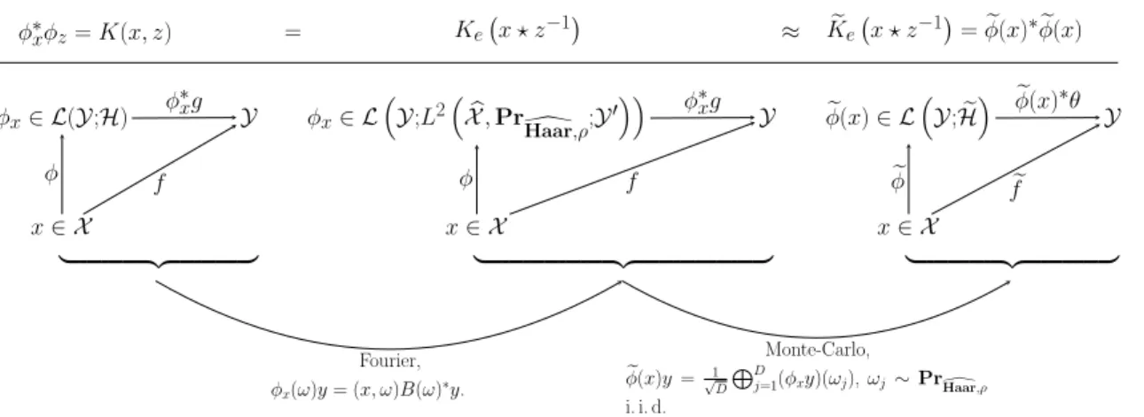
𝜑𝑥∈ ℒ(𝒴;ℋ) 𝒴 𝜑𝑥∈ ℒ (︁ 𝒴;𝐿2(︁𝒳 , Pr̂︀ \ Haar,𝜌;𝒴 ′)︁)︁ 𝒴 ̃︀ 𝜑(𝑥) ∈ ℒ (︁ 𝒴; ̃︀ℋ)︁ 𝒴 𝑥 ∈ 𝒳 𝑥 ∈ 𝒳 𝑥 ∈ 𝒳 𝜑*𝑥𝑔 𝑓 𝜑 𝜑*𝑥𝑔 𝑓 𝜑 ̃︀ 𝜑(𝑥)*𝜃 ̃︀ 𝑓 ̃︀ 𝜑 ⎫ ⎪ ⎪ ⎪ ⎪ ⎪ ⎪ ⎪ ⎪ ⎬ ⎪ ⎪ ⎪ ⎪ ⎪ ⎪ ⎪ ⎪ ⎭ ⎭⎪⎪⎪⎪⎪⎪⎪⎪⎪⎪⎪⎪⎪⎪⎪ ⎬⎪⎪⎪⎪⎪⎪⎪⎪⎪⎪⎪⎪⎪⎪⎪ ⎫ ⎭⎪⎪⎪⎪⎪⎪⎪⎪⎪ ⎬⎪⎪⎪⎪⎪⎪⎪⎪⎪ ⎫ 𝜑*𝑥𝜑𝑧= 𝐾(𝑥, 𝑧) = 𝐾𝑒(︀𝑥 ⋆ 𝑧−1)︀ ≈ 𝐾̃︀𝑒(︀𝑥 ⋆ 𝑧−1)︀ =𝜑(𝑥)̃︀ *𝜑(𝑥)̃︀ Fourier, 𝜑𝑥(𝜔)𝑦 = (𝑥, 𝜔)𝐵(𝜔)*𝑦. Monte-Carlo, ̃︀ 𝜑(𝑥)𝑦 =√1 𝐷 ⨁︀𝐷 𝑗=1(𝜑𝑥𝑦)(𝜔𝑗), 𝜔𝑗∼ PrHaar,𝜌\ i. i. d.
Figure 4: Relationships between feature-maps. For any realization of 𝜔𝑗 ∼ PrHaar,𝜌\ i. i. d., ̃︀
ℋ =⨁︀𝐷 𝑗=1𝒴′.
that for all 𝑦 ∈ 𝒴 and all 𝑦′ ∈ 𝒴′, ⟨𝑦, 𝐵(·)𝑦′⟩ ∈ 𝐿2( ̂︀𝒳 , Pr \
Haar,𝜌), then the operator-valued function ̃︀𝜑 : 𝒳 → ℒ
(︁ 𝒴,⨁︀𝐷
𝑗=1𝒴
′)︁defined for all 𝑥 ∈ 𝒳 and for all 𝑦 ∈ 𝒴 by
(16 ) ̃︀ 𝜑(𝑥)𝑦 = √1 𝐷 𝐷 ⨁︁ 𝑗=1 (𝑥, 𝜔𝑗)𝐵(𝜔𝑗)*𝑦, 𝜔𝑗 ∼ PrHaar,𝜌\ , i. i. d.,
is an approximated feature map of some 𝒴-Mercer operator-valued kernel4.
The difference between Proposition 22 and Proposition 19 is that in Proposition 22 we do not assume that 𝐴(𝜔) and Pr𝐻𝑎𝑎𝑟,𝜌\ have been obtained from Proposition 17. We conclude by showing that any realization of an approximate feature map gives a proper operator valued kernel. Hence we can always view ˜𝐾(𝑥, 𝑧) = ̃︀𝜑(𝑥)*𝜑(𝑧) —where ̃︀̃︀ 𝜑 is defined as in Proposition 18 (construction from an OVK) or Proposition 22— as a 𝒴-Mercer and thus apply all the classic results of the Operator-Valued Kernel theory on ˜𝐾.
Proposition 23
Let 𝜔 ∈ 𝒳̂︀𝐷. If for all 𝑦, 𝑦′ ∈ 𝒴 ⟨𝑦′, ̃︀𝐾𝑒(︀𝑥 ⋆ 𝑧−1)︀ 𝑦⟩𝒴 = ⟨ ̃︀𝜑(𝑥)𝑦′, ̃︀𝜑(𝑧)𝑦⟩ ̃︀ ℋ = ⟨ 𝑦′,𝐷1 ∑︀𝐷 𝑗=1(𝑥 ⋆ 𝑧−1, 𝜔𝑗)𝐵(𝜔𝑗)𝐵(𝜔𝑗) *𝑦⟩
𝒴, for all 𝑥, 𝑧 ∈ 𝒳 , then ̃︀𝐾 is a shift-invariant 𝒴-Mercer Operator-Valued Kernel.
Note that the above theorem does not consider the 𝜔𝑗’s as random variables and therefore does not shows the convergence of the kernel ̃︀𝐾 to some target kernel 𝐾. However is shows that any realization of ̃︀𝐾 when 𝜔𝑗’s are random variables yields a valid 𝒴-Mercer operator-valued kernel. Note that the above theorem does not considers the 𝜔𝑗’s as random variables and therefore does not shows the convergence of the kernel ̃︀𝐾 to some target kernel 𝐾. However is shows that any realization of ̃︀𝐾 when 𝜔𝑗’s are random variables yields a
4. i. e. it satisfies ̃︀𝜑(𝑥)*𝜑(𝑧)̃︀ a. s. −−−−→
valid 𝒴-Mercer operator-valued kernel. Indeed, as a result of Proposition 23, in the same way we defined an ORFF, we can define an approximate feature operator ̃︁𝑊 which maps ̃︀ℋ onto ℋ ̃︀ 𝐾, where ̃︀𝐾(𝑥, 𝑧) = ̃︀𝜑(𝑥) * ̃︀ 𝜑(𝑧), for all 𝑥, 𝑧 ∈ 𝒳 . Definition 24 (Random Fourier feature operator)
Let 𝜔 = (𝜔𝑗)𝐷𝑗=1∈ ̂︀𝒳𝐷 and let ̃︀𝐾𝑒= 𝐷1 ∑︀𝐷𝑗=1(·, 𝜔𝑗)𝐵(𝜔𝑗)𝐵(𝜔𝑗)*. We call random Fourier feature operator the linear application ̃︁𝑊 : ̃︀ℋ → ℋ
̃︀ 𝐾 defined as (︁ ̃︁ 𝑊 𝜃)︁(𝑥) : = ̃︀𝜑(𝑥)*𝜃 = √1 𝐷 𝐷 ∑︁ 𝑗=1 (𝑥, 𝜔𝑗)𝐵(𝜔𝑗)𝜃𝑗 where 𝜃 = ⨁︀𝐷
𝑗=1𝜃𝑗 ∈ ℋ.̃︀ Then from Proposition 6, (︁ Ker ̃︁𝑊 )︁⊥ = span {︁ ̃︀ 𝜑(𝑥)𝑦 ⃒ ⃒ ⃒∀𝑥 ∈ 𝒳 , ∀𝑦 ∈ 𝒴 }︁ ⊆ ̃︀ℋ.
The random Fourier feature operator is useful to show the relations between the random Fourier feature map with the functional feature map defined in Proposition 21. The relationship between the generic feature map (defined for all Operator-Valued Kernel) the functional feature map (defining a shift-invariant 𝒴-Mercer Operator-Valued Kernel) and the random Fourier feature map is presented in Figure 4.
Proposition 25 For any 𝑔 ∈ ℋ = 𝐿2( ̂︀𝒳 , Pr \ Haar,𝜌; 𝒴 ′), let 𝜃 := √1 𝐷 ⨁︀𝐷 𝑗=1𝑔(𝜔𝑗), 𝜔𝑗 ∼ PrHaar,𝜌\ i. i. d. Then 1. (︁̃︁𝑊 𝜃 )︁ (𝑥) = ̃︀𝜑(𝑥)*𝜃−−−−→a. s. 𝐷→∞ 𝜑 * 𝑥𝑔 = (𝑊 𝑔)(𝑥), 2. ‖𝜃‖2 ̃︀ ℋ a. s. −−−−→ 𝐷→∞ ‖𝑔‖ 2 ℋ, We write ̃︀𝜑(𝑥)*𝜑(𝑥) ≈ 𝐾(𝑥, 𝑧) when ̃︀̃︀ 𝜑(𝑥)*𝜑(𝑥)̃︀ a. s.
−−→ 𝐾(𝑥, 𝑧) in the weak operator topology when 𝐷 tends to infinity. With mild abuse of notation we say that ̃︀𝜑(𝑥) is an approximate feature map of the functional feature map 𝜑𝑥 i. e. ̃︀𝜑(𝑥) ≈ 𝜑𝑥, when for all 𝑦′, 𝑦 ∈ 𝒴,
⟨𝑦, 𝐾(𝑥, 𝑧)𝑦′⟩𝒴 = ⟨𝜑𝑥𝑦, 𝜑𝑧𝑦′⟩𝐿2( ̂︀𝒳 ,Pr \ Haar,𝜌;𝒴 ′) ≈ ⟨ ̃︀𝜑(𝑥)𝑦, ̃︀𝜑(𝑥)𝑦 ′⟩ ̃︀ ℋ := ⟨𝑦, ˜𝐾(𝑥, 𝑧)𝑦 ′⟩ 𝒴
where 𝜑𝑥 is defined in the sense of Proposition 21.
3.5 Examples of Operator Random Fourier Feature maps
We now give two examples of operator-valued random Fourier feature map. First we introduce the general form of an approximated feature map for a matrix-valued kernel on the additive group (R𝑑, +).
In the following let 𝐾(𝑥, 𝑧) = 𝐾0(𝑥 − 𝑧) be a 𝒴-Mercer matrix-valued kernel on 𝒳 = R𝑑, invariant w. r. t. the group operation +. Then the function ̃︀𝜑 defined as follow is an Opera-tor-valued Random Fourier Feature of 𝐾0. For all 𝑦 ∈ 𝒴,
̃︀ 𝜑(𝑥)𝑦 = √1 𝐷 𝐷 ⨁︁ 𝑗=1 (︃ cos ⟨𝑥, 𝜔𝑗⟩2𝐵(𝜔𝑗)*𝑦 sin ⟨𝑥, 𝜔𝑗⟩2𝐵(𝜔𝑗)*𝑦 )︃ , 𝜔𝑗 ∼ PrHaar,𝜌\ i. i. d..
In particular we deduce the following features maps for the kernels proposed in Subsection 3.2. ∙ For the decomposable Gaussian kernel 𝐾0𝑑𝑒𝑐,𝑔𝑎𝑢𝑠𝑠(𝛿) = 𝑘𝑔𝑎𝑢𝑠𝑠0 (𝛿)Γ for all 𝛿 ∈ R𝑑, let
𝐵𝐵* = Γ. A bounded –and unbounded– ORFF map is
̃︀ 𝜑(𝑥)𝑦 = √1 𝐷 𝐷 ⨁︁ 𝑗=1 (︃ cos ⟨𝑥, 𝜔𝑗⟩2𝐵*𝑦 sin ⟨𝑥, 𝜔𝑗⟩2𝐵*𝑦 )︃ = (𝜙(𝑥) ⊗ 𝐵̃︀ * )𝑦, where 𝜔𝑗 ∼ Pr𝒩 (0,𝜎−2𝐼 𝑑) i. i. d. and 𝜙(𝑥) =̃︀ 1 √ 𝐷 ⨁︀𝐷 𝑗=1 (︃ cos ⟨𝑥, 𝜔𝑗⟩2 sin ⟨𝑥, 𝜔𝑗⟩2 )︃ is a scalar RFF map (Rahimi and Recht, 2007).
∙ For the curl-free Gaussian kernel, 𝐾0𝑐𝑢𝑟𝑙,𝑔𝑎𝑢𝑠𝑠= −∇∇T𝑘𝑔𝑎𝑢𝑠𝑠0 an unbounded ORFF map is (17) ̃︀ 𝜑(𝑥)𝑦 = √1 𝐷 𝐷 ⨁︁ 𝑗=1 (︃ 𝑔 cos ⟨𝑥, 𝜔𝑗⟩2𝜔T𝑗𝑦 sin ⟨𝑥, 𝜔𝑗⟩2𝜔T𝑗𝑦 )︃ , 𝜔𝑗 ∼ Pr𝒩 (0,𝜎−2𝐼
𝑑) i. i. d. and a bounded ORFF map is
̃︀ 𝜑(𝑥)𝑦 = √1 𝐷 𝐷 ⨁︁ 𝑗=1 ⎛ ⎝ cos ⟨𝑥, 𝜔𝑗⟩2 𝜔T 𝑗 ‖𝜔𝑗‖𝑦 sin ⟨𝑥, 𝜔𝑗⟩2 𝜔T𝑗 ‖𝜔𝑗‖𝑦 ⎞ ⎠, 𝜔𝑗 ∼ Pr𝜌 i. i. d..
where 𝜌(𝜔) = 𝜎2‖𝜔‖𝑑 2𝒩 (0, 𝜎−2𝐼𝑑)(𝜔) for all 𝜔 ∈ R𝑑.
∙ For the divergence-free Gaussian kernel 𝐾0𝑑𝑖𝑣,𝑔𝑎𝑢𝑠𝑠(𝑥, 𝑧) = (∇∇T− Δ𝐼𝑑)𝑘𝑔𝑎𝑢𝑠𝑠0 (𝑥, 𝑧) an unbounded ORFF map is
(18) ̃︀ 𝜑(𝑥)𝑦 = √1 𝐷 𝐷 ⨁︁ 𝑗=1 (︃ cos ⟨𝑥, 𝜔𝑗⟩2𝐵(𝜔𝑗)T𝑦 sin ⟨𝑥, 𝜔𝑗⟩2𝐵(𝜔𝑗)T𝑦 )︃
where 𝜔𝑗 ∼ Pr𝜌i. i. d. and 𝐵(𝜔) =(︀‖𝜔‖𝐼𝑑− 𝜔𝜔T)︀ and 𝜌 = 𝒩 (0, 𝜎−2𝐼𝑑) for all 𝜔 ∈ R𝑑. A bounded ORFF map is
̃︀ 𝜑(𝑥)𝑦 = √1 𝐷 𝐷 ⨁︁ 𝑗=1 𝑔 (︃ cos ⟨𝑥, 𝜔𝑗⟩2𝐵(𝜔𝑗)T𝑦 sin ⟨𝑥, 𝜔𝑗⟩2𝐵(𝜔𝑗)T𝑦 )︃ , 𝜔𝑗 ∼ Pr𝜌 i. i. d., where 𝐵(𝜔) =(︁𝐼𝑑− 𝜔𝜔 T ‖𝜔‖2 )︁ and 𝜌(𝜔) = 𝜎2‖𝜔‖𝑑 2𝒩 (0, 𝜎−2𝐼 𝑑) for allg 𝜔 ∈ R𝑑.