An Efficient Mechanism for Processing Top-k Queries in DHTs

HAL Id: inria-00482363

https://hal.inria.fr/inria-00482363

HAL is a multi-disciplinary open access archive for the deposit and dissemination of sci-entific research documents, whether they are pub-lished or not. The documents may come from teaching and research institutions in France or abroad, or from public or private research centers.

L’archive ouverte pluridisciplinaire HAL, est destinée au dépôt et à la diffusion de documents scientifiques de niveau recherche, publiés ou non, émanant des établissements d’enseignement et de recherche français ou étrangers, des laboratoires publics ou privés.

An Efficient Mechanism for Processing Top-k Queries in

DHTs

Reza Akbarinia, Esther Pacitti, Patrick Valduriez

To cite this version:

Reza Akbarinia, Esther Pacitti, Patrick Valduriez. An Efficient Mechanism for Processing Top-k Queries in DHTs. BDA: Bases de Données Avancées, Oct 2006, Lille, France. �inria-00482363�

An Efficient Mechanism for Processing Top-k Queries in DHTs

Reza Akbarinia Esther Pacitti Patrick Valduriez

Atlas team, INRIA and LINA University of Nantes, France

{FirstName.LastName@univ-nantes.fr, Patrick.Valduriez@inria.fr}

1 _{Work partially funded by the ARA Massive Data of the Agence Nationale de la Recherche.}

Abstract

We consider the problem of top-k query processing in Distributed Hash Tables (DHTs). The most efficient approaches for top-k query processing in centralized and distributed systems are based on the Threshold Algorithm (TA) which is applicable for queries where the scoring function is monotone. However, the specific interface of DHTs, i.e. data storage and retrieval based on keys, makes it hard to develop TA-style top-k query processing algorithms. In this paper, we propose an efficient mechanism for top-k query processing in DHTs. It is widely applicable to many different DHT implementations. Although our algorithm is TA-style, it is much more general since it supports a large set of non monotone scoring functions including linear functions. In fact, it is the first TA-style algorithm that supports linear scoring functions. We prove analytically the correctness of our algorithm. We have validated our algorithm through a combination of implementation and simulation. The results show very good performance, in terms of communication cost and response time.

Keywords: DHT, Query processing, Top-k queries.

1.

Introduction

Distributed Hash Tables (DHTs), e.g. CAN [26], Chord [31], Tapestry [33] and Pastry [28], provide an efficient solution for data location and lookup in large-scale P2P systems. While there are significant implementation differences between DHTs, they all map a given key onto a peer p using a hash function and can lookup p efficiently, usually in O(log n) routing hops where n is the number of peers [12][17]. DHTs typically provide two basic operations [17][27]:

put(key, data) stores a pair (key, data) in the

DHT using some hash function; get(key) retrieves the data associated with key in the

DHT. These operations enable supporting exact-match queries only. Recently, much work has been devoted to supporting more complex queries on top of DHTs such as range queries [15] [17] and join queries[20]. However, efficient evaluation of more complex queries in DHTs is still an open problem.

An important kind of complex queries is top-k queries. A top-top-k query specifies a number top-k of the most relevant answers desired together with a scoring function that expresses the degree of relevance (score) of the answers. Top-k queries have attracted much interest in many different areas such as network and system monitoring [2][21][9], information retrieval [22][6][30][25], multimedia databases [10][24][13][16], spatial data analysis [7][11][18], etc. The main reason for such interest is that they avoid overwhelming the user with large numbers of uninteresting answers which are resource-consuming. In a large-scale P2P system, top-k queries can be very useful [6]. For example, consider a P2P system with medical doctors who want to share some (restricted) patient data for an epidemiological study. Assume that all doctors agreed on a common Patient description in relational format. Then, one doctor may want to submit the following query over the P2P system to obtain the 10 top answers ranked by a scoring function over height and weight:

SELECT *

FROM Patient P

WHERE (P.disease = “diabetes”) AND (P.height < 170) AND (P.weight > 70) ORDER BY scoring-function(height, weight) STOP AFTER 10

The scoring function specifies how closely each data item matches the conditions. For instance, in the query above, the scoring function could be (weight - (height -100)) which computes the overweight.

The most efficient approaches for top-k query processing in centralized and distributed systems

are based on the Threshold Algorithm (TA) [14][16][24]. TA is applicable for queries where the scoring function is monotone, i.e., any increase in the value of the input does not decrease the value of the output. Many of the popular aggregation functions, e.g. Min, Max, Average, are monotone. However, there are many useful functions that are not monotone including most of linear functions, e.g. the function of the above example. TA works as follows. Given m lists of n objects such that each object has a local score in each list and the lists are sorted according to the local scores of their objects, TA finds k objects whose overall scores are the highest. The overall score of an object is computed based on the local scores of the object in all lists using the scoring function. TA goes down the sorted lists in parallel, one position at a time, and for each seen object, computes its overall score. This process continues until finding k objects whose overall scores are greater than a threshold which is computed based on the local score of the objects at current position.

TA-style algorithms, i.e. algorithms inspired from TA, are fairly well developed for top-k query processing in centralized data management systems, but much less in distributed systems such as P2P federations [23]. In particular, the specific interface of DHTs, i.e. data storage and retrieval based on keys, makes it hard to develop TA-style top-k query processing algorithms.

In this paper, we propose an efficient mechanism for top-k query processing in DHTs. It is widely applicable to many different DHT implementations such as CAN, Chord, Tapestry and Pastry. To the best of our knowledge, this is the first paper that addresses the problem of efficient top-k query processing in DHTs. Although our algorithm is TA-style, it is much more general than TA since it supports a large set of non monotone scoring functions including linear functions. For instance, it can support the function of the above example, i.e. (weight - (height - 100)), which is not monotone and cannot be processed by TA. In fact, our algorithm is also the first TA-style algorithm that supports linear scoring functions. We prove analytically the correctness of our algorithm. We have also validated our algorithm through a combination of implementation and simulation and the results show very good performance, in terms of communication cost and response time.

This work is done in the context of APPA (Atlas Peer-to-Peer Architecture) [3][4], a P2P data management system which we are building. The main objectives of APPA are scalability, availability and performance for advanced applications.

The rest of this paper is organized as follows. In Section 2, we give a precise definition of the problem based on the definition of the set of scoring functions which we support. In Section 3, we present our mechanism for storing the shared data in a DHT. In Section 4, we present our algorithm for processing top-k queries in DHTs. Section 5 describes a performance evaluation of our algorithm through implementation over a 64-node cluster and simulation using SimJava [18]. Section 6 discusses related work and Section 7 concludes.

2.

Problem Definition

In this section, we first define the scoring functions that our algorithm supports. Then, we make precise our assumptions and state the problem we address in this paper.

2.1 Supported Scoring Functions

Let f be a scoring function that given values x1, x2, .., xm for its variables X1, X2 …, Xm returns a real number as the score of the given values. Monotonic scoring functions are defined as follows [14].

Definition 1 (Monotonic scoring function): f is

monotonic if f(x1, x2, …, xm) ≤ f(x'1, x'2, …, x'm)

whenever xj≤ x'j for every j. In other words,

increasing the value of variables does not decrease the output of the scoring function.

Monotonic scoring functions are very useful in practice. Aggregate functions such as MIN, MAX and AVERAGE are monotonic. However, there are many functions that are not monotonic, for instance f(X1, X2) = X1 – X2 is not monotonic,

e.g. f(6, 6) > f(7, 8). In fact, no linear function is

monotonic unless the quotient of all variables is positive.

Our solution supports a set of scoring functions, which we denote as IOD-EV, and which is a super set of monotonic scoring functions. To define IOD-EV functions, we need the two following definitions.

Definition 2 (Increasing wrt variable Xi): A

scoring function f is increasing wrt variable Xi if

f(x1, x2,…, xi-1, xi, xi+1,…, xm) f(x1, x2,…, xi-1, x'i,

increasing the value of variable Xi does not

decrease the output of the scoring function.

Definition 3 (Decreasing wrt variable Xi): A

scoring function f is decreasing wrt variable Xi,

if f(x1, x2,…, xi-1, xi, xi+1,…, xm) ≥ f(x1, x2,…, xi-1,

x'i, xi+1,…, xm) whenever xi≤ x'i. In other words,

increasing the value of variable Xi does not

increase the output of the scoring function.

For example the function f(X1, X2) = X1 – X2 is increasing wrt X1 and decreasing wrt X2. Now we can define IOD-EV scoring functions.

Definition 4 (Increasing Or Decreasing wrt Each Variable (IOD-EV)): A scoring function f

is IOD-EV if for each variable Xi, f is increasing

wrt Xi or decreasing wrt Xi.

For example, the functions f(X1, X2) = X1 – X2 and f(X1, X2) = (X1)3 – (X2)3 are IOD-EV. The set of monotonic scoring functions is a subset of IOD-EV functions as shown below.

Lemma 1: Every monotonic scoring function is

IOD-EV.

Proof: A monotonic scoring function is increasing wrt every variable, thus it is IOD-EV. The linear functions are also IOD-EV as demonstrated below.

Lemma 2: Every linear function is IOD-EV. Proof: A linear function can be written as f(X1,

X2, …, Xm) = a0 + a1X1 + a2X2 + …+ amXm where

a0, a1, …, am are constant values. For each variable Xi if its quotient ai is positive then f is increasing wrt Xi, otherwise it is decreasing wrt

Xi. Thus, all linear functions are IOD-EV.

2.2 Problem Statement

In this paper, we assume relational data, i.e. tuples. For simplicity, we assume top-k queries with no join operation. We also assume that the scoring function specified in the query is IOD-EV. Our objective is to find the k highest scored tuples from the tuples that are stored in the DHT and satisfy Q’s conditions. Formally, let Q be a top-k query issued at some peer, and T be the set of tuples that are stored in the DHT and satisfy the qualification of Q. Let sc(t) be the scoring function that is specified in Q and determines the score of a given tuple t∈T. Our goal is to find

efficiently the set Ttk⊆ T such that: Ttk = k and

∀ t1∈ Ttk,∀ t2 ∈ (T - Ttk) we have sc(t1) ≥ sc(t2).

3.

Data Storage Mechanism

In this section, we propose our mechanism for storing relational data in the DHT. This mechanism not only provides good support for exact-match queries, it also enables efficient execution of our top-k query processing algorithm.

Our data storage mechanism relies on a Persistent Data Management service (PDM) [4][4] which provides high availability for (key, data) pairs stored in the DHT. The PDM service provides: a put(key, data) operation that replicates a (key, data) pair at several peers using several hash functions, and a get(key) operation that retrieves one of the available replicas of a data that is stored with key in the DHT. Using PDM, even with high churn of peers, we have a very high chance to retrieve data from the DHT. In the rest of this paper, the key used for storing a data in the DHT is called the storage key of that data.

In our data storage mechanism, peers store their relational data in the DHT with two complementary methods: tuple storage and attribute-value storage.

3.1 Tuple Storage

With the tuple storage method, each tuple of a relation is entirely stored in the DHT using its tuple identifier (e.g. its primary key) as the storage key. This enables looking up a tuple by its identifier. Let R be a relation name and A be the set of its attributes. Let T be the set of tuples of R and id(t) be a function that denotes the identifier of a tuple t∈T. Let h be a hash function

that hashes its inputs into a DHT key, i.e. a number which can be mapped by the DHT onto a peer. For storing relation R, each tuple t∈T is

entirely stored in the DHT where the storage key is h(R, id(t)), i.e. the hash of the relation name and the tuple identifier. In other word, for storing

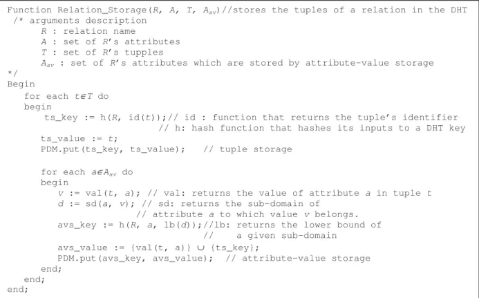
R, the following instructions are done (see Figure

1): ∀ t∈ T, put(h(R, id(t)), { t })

Hereafter, we denote h(R, id(t)) by ts_key(t) and call it tuple storage key.

3.2 Attribute Value Storage

The attribute-value storage method enables answering exact-match queries. In addition to tuple storage, the attributes that may appear in a query’s “where” clause, are stored individually in the DHT, like in database secondary indexes.

Figure 1. Storing a relation in the DHT

These attributes include those used in equality predicates or passed as arguments to the scoring function. Let Aav∈A be the set of R’s attributes

which are stored using attribute-value storage. Let val(t, a) be a function that returns the value of an attribute a in a tuple t. With attribute-value storage, for every t∈T and for each a∈Aav we store in the DHT a set containing val(t, a) and

ts_key(t) (see Figure 1). The reason, for which

upon attribute-value storage we store ts_key(t), is that it enables us to retrieve the entire tuple after retrieving one of its values which are stored through attribute-value storage.

The storage key used for attribute-value storage, denoted by avs_key and called

attribute-value storage key, is determined in such a way

that, for the values of an attribute that are relatively “close”, avs_key is the same.

To determine avs_key, we use the concept of domain partitioning. Consider an attribute a∈Aav and let Da be its domain of values. Assume there is a total order < on Da, e.g. Da is numeric, string, date, etc. We partition Da into n nonempty sub-domains d1, d2, …, dn such that their union is equal to Da, the intersection of any two different

sub-domains is empty, and for each v1∈di and

v2∈dj, if i<j then we have v1<v2. For example, attribute “weight”, whose domain is [0..200] in kilograms, can be partitioned into 40

sub-domains [0..5), [5..10), …, [190..195), [195..200]. The lower bound of each sub-domain

dis denoted by lb(d). Given a value v, the sub-domain to which v belongs is denoted by sd(a,

v). The number of sub-domains of an attribute

and the lower bound of each sub-domain are known to all peers of the DHT. Therefore, given an attribute a and a value v, any peer can locally compute sd(a, v).

Using domain partitioning, the attribute-value storage key, i.e. avs_key, can be computed as follows. Let R be a relation name, a∈Aav be an attribute, and v be a value of a, the attribute-value storage key for storing v in the DHT is h(R,

a, lb(sd(a, v))), i.e. the hash of the relation name,

attribute name and the lower bound of the sub-domain to which v belongs. Thus, for the values of an attribute that belong to the same sub-domain, avs_key is the same key, so those values are stored at the same peer.

Partitioning the domain of an attribute allows us to store the attribute values which belong to the same sub-domain at the same peer. The partitioning can be done by the designers of the DHT application or by the owners of the relations at schema mapping time.

However, the partitioning method used should also avoid attribute storage skew, i.e. skewed distribution of attribute values within

Function Relation_Storage(R, A, T, Aav)//stores the tuples of a relation in the DHT

/* arguments description R : relation name

A : set of R’s attributes T : set of R’s tupples

Aav : set of R’s attributes which are stored by attribute-value storage

*/ Begin

for each t∈T do

begin

ts_key := h(R, id(t));// id : function that returns the tuple’s identifier // h: hash function that hashes its inputs to a DHT key

ts_value := t;

PDM.put(ts_key, ts_value); // tuple storage

for each a∈Aav do

begin

v := val(t, a); // val: returns the value of attribute a in tuple t d := sd(a, v); // sd: returns the sub-domain of

// attribute a to which value v belongs. avs_key := h(R, a, lb(d));//lb: returns the lower bound of

// a given sub-domain avs_value := {val(t, a)} ∪ {ts_key};

PDM.put(avs_key, avs_value); // attribute-value storage end;

end; end;

sub-domains, which may yield load unbalancing among peers. For instance, simply dividing the domain into n equal-width sub-domains, as we did for attribute “weight” above, may yield attribute storage skew, e.g. with a much larger partition for the weight sub-domains between 60 and 80.

If at partitioning time, we have histogram-based information that describe the distribution of the values of an attribute, we can do a better partitioning such that the values be uniformly distributed within the sub-domains. Formally, let

pa(v) be the probability density function that describes the probability that attribute a takes a value equal to v. To obtain a uniform partitioning, we choose the lower bound of sub-domains d1, d2, …, dn such that:

n

dv

v

p

1

)

(

=

By these n-1 equations, the sub-domains are constrained to have the same density of values. We know that the lower bound of d1 is equal to the lower bound of Da, so lb(d1) is determined.

Thus, we have n-1 equations with n-1 variables, i.e. lb(d2),…, lb(dn), and by solving the equations we can determine the value of lb(d2),…, lb(dn).

The partitioning of an attribute’s domain must be done before storing any value of the attribute in the DHT. After storing some attribute values in the DHT, it is no longer allowed to modify the number of sub-domains and their lower bounds since any modification may result in losing the ability to retrieve the stored attribute values, i.e. it may result in a new storage key for an stored attribute value which is different from the storage key by which the attribute value has been stored in the DHT.

4.

Top-k Query Processing

In this section, we propose DHTop, an algorithm for processing top-k queries in DHTs. We first present an overview of the algorithm, and then describe its phases in more details. Then, we prove its correctness. Finally, we present two optimizing strategies to further reduce the response time and communication cost of DHTop.

4.1 Algorithm Overview

DHTop works as follows. Let scoring attributes be the attributes that are passed to the scoring function as arguments. For each scoring

attribute, DHTop retrieves their values in parallel, one by one in order of their positive impact on the scoring function. Thus, the values for which the scoring function is higher are retrieved first. For each value retrieved, DHTop retrieves the entire tuple and computes the score of the tuple. The retrieval of attribute values continues until retrieving k tuples whose scores are greater than a threshold which is computed based on the last retrieved values using the scoring function. The threshold value is computed as in the TA algorithm.

To retrieve the values of the scoring attributes, DHTop proceeds as follows. For each scoring attribute, it creates a list of the attribute’s sub-domains, and orders them according to their positive impact on the scoring function, i.e. the sub-domains for which the scoring function is higher are at the beginning of the list. Then, starting from the head of the list, DHTop selects a sub-domain and requests the peer responsible for it to return the stored attribute values, one by one, in order of their positive impact on the scoring function. If the values which are stored at the first sub-domain of the list are not sufficient for finding the k top tuples, DHTop selects the second sub-domain, and requests its responsible to return its stored values. This process continues until finding k tuples whose scores are greater than the threshold.

Let Q be a given top-k query, f be its scoring function, Asf be the set of scoring attributes, and

pint be the peer at which Q is issued. We assume that f is IOD-EV. DHTop starts at pint and proceeds in four phases: (1) Prepare lists of candidate sub-domains; (2) Retrieve candidate attribute values; (3) Retrieve candidate tuples; and (4) Check the end condition.

4.2 Prepare Lists of Candidate Sub-domains

In this phase, for each scoring attribute, pint prepares a list of sub-domains and orders them according to their positive impact on the scoring function. These lists are used in the next phase for retrieving the values of scoring attributes. This phase proceeds as follows. For each attribute α∈Asf, pint creates a Candidate

sub-Domain List, denoted by CDLα, and performs the following steps:

Step 1: Initialization. pint initializes CDLα to contain all α’s sub-domains.

Step 2: Removing useless sub-domains. In this step, pint removes from CDLα the sub-domains of which no member can satisfy Q’s conditions. Without loss of generality, assume that Q is in conjunctive normal form. Depending on Q’s conditions, many of the sub-domains involved in

CDLα may be removed from it. In particular, this is true when some of Q’s conditions are the following:

• Bound Conditions. These are the conditions

that limit the attribute α to be lower or greater than a constant value, e.g. the condition α < u where u is a constant. For

each bound condition on α, pint removes from CDLα the sub-domains that are excluded by the bound condition. For example, for the condition α < u, pint removes from CDLα each sub-domain d such that lb(d) > u.

• Point Conditions. These are the conditions

that enforce the attribute α to be equal to a constant, e.g. α = u. For a point condition on

α, pint removes from CDLα all its sub-domains except the sub-domain to which the constant value belongs.

Step 3: Ordering candidate sub-domains. If the scoring function f is increasing wrt α then pint sorts CDLα in descending order of the lower bound of its involved sub-domains. Otherwise, it sorts CDLα in ascending order. Let CDLα[i] denote the ith sub-domain of CDLα. At the end of this step, CDLα is as follows. If f is increasing wrt α then lb(CDLα[i-1]) ≥ lb(CDLα[i]) whenever i>1. And if f is decreasing wrt α then

lb(CDLα[i-1]) ≤ lb(CDLα[i]) whenever i>1.

4.3 Retrieve Candidate Attribute Values

The objective of this phase is to retrieve the stored values of the scoring attributes, in order of their positive impact on the scoring function.

In this phase, for each attribute α∈Asf in parallel, pint performs as follows. It sends Q and

α to the peer, say p, that is responsible for storing the values of the first sub-domain of

CDLα, and requests it to return the values of α that are stored at p. The values are returned in order of their positive impact on the scoring function. If the values that p returns to pint are not sufficient for determining the k top tuples, pint sends Q and α to the responsible of the second sub-domain of CDLα. This process continues until the end condition holds and the algorithm ends.

The details of the actions, which are done by

p after receiving the request of pint, are as follows. Let Vα be the list of all values of the attribute α that are stored at p, it creates a

Candidate Attribute Value List for α, denoted by

CAVLα, and performs the following steps:

Step 1: Initialization. p initializes CAVLα to contain all values involved in Vα.

Step 2: Removing useless sub-domains. p removes from CAVLα the values that are excluded by Q’s conditions, in particular bound and point conditions similar to Step 2 in the previous phase.

Step 3: Ordering candidate values. If the scoring function f is increasing wrt α then p sorts

CAVLα in descending order. Otherwise, it sorts it in ascending order.

Step 4: Sending the candidate values to pint

sequentially. In this step, p starts sending the values involved in CAVLα to pint, one by one, and from the head of CAVLα to its end, until arriving at the end of CAVLα or receiving the “end” message from pint. Along with each value, its tuple storage key (i.e. ts_key) which is stored with the value upon attribute-value storage (see Section 3.2), and its index in CAVLαare also sent to pint.

It is needed that pint receives the values sent by p in their sending sequence. For this, when

pint receives a value v, it compares its index, say

i, with the index of the last received value, say j.

If i=j+1 then it considers v as a retrieved

attribute value, otherwise it discards v and asks p

to send the values from the index j+1.

4.4 Retrieve Candidate Tuples

The objective of this phase is to retrieve the tuple of each retrieved attribute value, compute the tuple’s score, and keep it if its score is one of the

k highest scores yet computed.

After retrieving each attribute value v, pint retrieves the tuple which v belongs to, say t, using ts_key(t) which is received along with v. If

t does not satisfy Q’s conditions, pint discards it. Otherwise it computes the score of t using the scoring function f. If this score is one of the k highest scores pint has yet computed, it adds t to the set Y (which has been initialized to empty). If

Y > k then it removes from Y the tuple with the

4.5 Check the End Condition

The objective of this phase, which is done by pint after retrieving each attribute value and its tuple, is to check whether there are at least k tuples (among the retrieved tuples) whose scores are greater than the threshold. If yes, the algorithm ends, otherwise it continues.

For each attribute ai∈Asf let vi be the last value received for ai, we define the threshold δ to be f(v1, v2, …, vm). After retrieving each attribute value and its tuple, pint computes δ. If Y =k and the score of all tuples involved in Y is at least

δ, then the end condition holds. In this case, for each attribute ai∈Asf, pint sends an “end” message to the peer that is sending the stored values of ai to pint. Then, the algorithm ends and the output is the set of tuples involved in Y.

4.6 Correctness

Let us now prove the correctness of the DHTop algorithm. For this, we prove the following lemma which will be used in the proof of Theorem 1.

Lemma 3: Let f be an IOD-EV scoring

function, vi and v'i be two stored values for an

scoring attribute ai such that vi is retrieved by

DHTop, and v'i is retrieved after vi or it is not

retrieved by DHTop, then we have f(x1, x2,…, xi-1,

v'i, xi+1,…, xm) ≤ f(x1, x2,…, xi-1, vi, xi+1,…, xm) for

any value xj ,1≤j≤m and j≠i.

Proof: With respect to the possible values vi

and v'i , there are two cases to consider. In the first case, vi and v'i belong to two different sub-domains, e.g. d1 and d2 respectively. Thus, d1 is before d2 in CDLai. If f is increasing wrt ai, then considering Step 3 of the first phase of the algorithm, we have lb(d1) ≥ lb(d2). Thus, we have vi ≥ v'i and since f is increasing wrt ai, we have f(x1, x2,…, xi-1, v'i, xi+1,…, xm) ≤ f(x1, x2,…,

xi-1, vi, xi+1,…, xm). Now, if f is decreasing wrt ai, then considering Step 3 of the first phase of the algorithm, we have lb(d1) ≤ lb(d2). Thus vi ≤ v'i and since f is decreasing wrt ai, we have f(x1, x2,…, xi-1, v'i, xi+1,…, xm) ≤ f(x1, x2,…, xi-1, vi,

xi+1,…, xm). The second case is when vi and v'i belong to the same sub-domain. It is obvious that

vi is before v'i in CAVLai. If f is increasing wrt ai, then considering Step 3 of the second phase of the algorithm, we have vi≥ v'i and thus f(x1, x2,…,

xi-1, v'i, xi+1,…, xm) ≤ f(x1, x2,…, xi-1, vi, xi+1,…,

xm). If f is decreasing wrt ai, we have vi≤ v'i and thus f(x1, x2,…, xi-1, v'i, xi+1,…, xm) ≤ f(x1, x2,…,

xi-1, vi, xi+1,…, xm).

Now, the following theorem provides the correctness of our algorithm.

Theorem 1: If f is an IOD-EV scoring

function, then DHTop finds the k top tuples correctly.

Proof: the proof is done by contradiction. Let

Y be the set of k top tuples obtained by DHTop,

and t' be the tuple in Y whose score is the lowest. We assume there is a tuple t''∉Y such that its

score is greater than t', and we show that this assumption yields to a contradiction. Let a1, a2,

…, am be the scoring attributes. Let v1, v2, …, vm be the last values, i.e. before ending the algorithm, retrieved respectively for attributes a1, a2, …, am. Let v'1, v'2, …, v'm be the values of the attributes a1, a2, …, am in t', respectively. Let v''1,

v''2, …, v''m be the value of attributes a1, a2, …, am in t'', respectively. Since t'' is not in Y, it was not retrieved during the execution of our algorithm. Thus, none of its values, i.e. v''1, v''2, …, v''m, was retrieved by pint, because if the value of any attribute of a tuple was retrieved, the entire tuple would have been retrieved by the algorithm. By applying Lemma 3 on attribute a1 we have f(v1, v2, …, vm) ≥ f(v''1, v2, …, vm). By applying the Lemma 3 on attribute a2, we have f(v''1, v2, v3,…,

vm) ≥ f(v''1, v''2, v3,…, vm). By continuing the application of Lemma 3 on attributes a3,…, am, we have f(v1, v2, …, vm) ≥ f(v''1, v2, …, vm) ≥ f(v''1,

v''2, …, vm) ≥… ≥ f(v''1, v''2, …, v''m-1, vm) ≥ f(v''1,

v''2, …, v''m-1, v''m). Therefore, we have f(v1, v2,

…, vm) ≥ f(v''1, v''2, …, v''m). According to the end condition of the algorithm, we have f(v'1, v'2, …,

v'm)≥ f(v1, v2, …, vm), and by comparing this inequality with the former one, we have f(v'1, v'2,

…, v'm)≥ f(v''1, v''2, …, v''m). In other words, the score of tuple t' is greater than that of t'', which yields to a contradiction.

4.7 Optimizing Strategies

We can further reduce response time and communication cost of DHTop. For this, we propose two simple optimizing strategies: batch retrieval of attribute values and retrieving each tuple at most once.

Batch retrieval of attribute values (BRAV). In Step 4 of Phase 2, the values of the scoring attributes are returned to pint one by one, i.e. each value in a message. Since each message has its own overhead, e.g. latency, returning only one value per message is very costly. To reduce such overhead, we can modify Step 4 of Phase 2 so that the peer p, which is responsible for storing

the values of a sub-domain, sends the attribute values to pint in a batch fashion, e.g. k values per message. In Section 5, we perform some experiments to study the effect of the number of values, which are sent per message, on response time.

Retrieving each tuple at most once (RTO). In the basic form of DHTop, after retrieving each value of a scoring attribute, the entire tuple of that value is retrieved. Since there may be several scoring attributes, a tuple may be retrieved several times. However, after the first retrieval of the tuple and comparing its score with the k highest scores, there is no need to retrieve it again because either the tuple is in the set Y or its score cannot be one of the k highest scores. Thus, to optimize our algorithm, we can change Phase 3 as follows. pint maintains a list of

ts_key of the tuples which have yet been

retrieved. Before retrieving a tuple t, pint checks the existence of ts_key(t) in the list. If it is not in the list then pint appends ts_key(t) to the list, and Phase 3 proceeds as described before, i.e. pint retrieves the tuple, computes its score, etc. Otherwise, pint does nothing, i.e. it does not retrieve the tuple.

5.

Performance Evaluation

We evaluated the performance of DHTop through implementation and simulation. The implementation over a 64-node cluster was useful to validate DHTop and calibrate our simulator. The simulator allows us to study scale up to high numbers of peers (up to 10,000 peers). The rest of this section is organized as follows. In Section 5.1, we describe our experimental and simulation setup, and the algorithms used for comparison. In Section 5.2, we first report experimental results using the implementation of four versions of our algorithm on a 64-node cluster, and then we present simulation results on performance by increasing the number of peers up to 10,000. In Sections 5.3, we evaluate the effect of the number of requested tuples, i.e. k, on performance. In Section 5.4, we vary the number of sub-domains to which an attributes domain is partitioned, and we investigate its effect on performance. In Section 5.5, we study the effect of data distribution on performance. In Section 5.6, we study the effect of the number of retrieved attribute values per message on the performance of the BRAV optimization.

5.1 Experimental and Simulation Setup

Our implementation is based on Chord [31] which is a simple and efficient DHT. Chord's lookup mechanism is provably robust in the face of frequent node failures and re-joins, and it can answer queries even if the system is continuously changing. We implemented PDM as a service on top of Chord which we also implemented. We also implemented our storage mechanism on top of Chord using PDM.

We tested our algorithms over a cluster of 64 nodes connected by a 1-Gbps network, that of the Paris team at IRISA2_{. Each node has 2 Intel}

Xeon 2.4 GHz processors, and runs the Linux operating system. We make each node act as a peer in the DHT.

To study the scalability of our algorithm far beyond 64 peers, we implemented a simulator using SimJava [19]. To simulate a peer, we use a SimJava entity that performs all tasks that must be done by a peer for executing DHTop. We assign a delay to communication ports to simulate the delay for sending a message between two peers in a real P2P system. Since the results gained from the simulator were similar to those gained from the implementation over the cluster, for most of our tests we only report simulation results.

Our default settings for different experimental parameters are shown in Table 1. Most of theses settings are the same as in [10]. In our tests, we use a synthetically generated relation with six attributes ai, 1≤i≤6 and the domain of the

attributes is numeric. The default number of tuples of the relation is 10,000 and they are randomly generated in two different ways: (1) Uniform data set, and (2) Gaussian data set. With (1), the values of attributes are independent of each other, and the distribution of the values of each attribute is uniform. This is our default setting. With (2), the values of different attributes are independent of each other, and the values for each attribute are generated via overlapping multidimensional Gaussian belles [32].

In our tests, the top-k query Q is delivered to a randomly selected peer. The selectivity of Q over the generated data is 10% and the scoring function specified in Q is the linear function f(a1, a2, a3, a4, a5, a6) = a1 – 2a2 + 3a3 – 4a4 + 5a5 –

6a6. Typically, users are interested in a small

number of top answers, thus we set k=10. In our storage mechanism, the domain of each attribute is uniformly partitioned into n sub-domains and the default value for n is 100.

The network parameters of the simulator are shown in Table 2. We use parameter values which are typical of P2P systems [29]. The latency between any two peers is a normally distributed random number with a mean of 200 (ms). The bandwidth between peers is also a random number with normal distribution with a mean of 56 (kbps). The simulator allows us to perform tests up to 10,000 peers, after which the simulation data no longer fit in RAM and makes our tests difficult. This is quite sufficient for our tests.

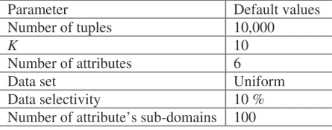
Table 1. Default setting of experimental parameters

Parameter Default values

Number of tuples 10,000

K 10

Number of attributes 6

Data set Uniform

Data selectivity 10 % Number of attribute’s sub-domains 100

Table 2. Network parameters of the simulator

Parameter Default values

Bandwidth Normally distributed random, Mean = 56 Kbps, Variance = 32

Latency Normally distributed random, Mean = 200 ms, Variance = 50 Number of peers 10,000 peers

To evaluate the performance of our algorithm, we measure the following metrics. 1) Response time: the time elapsed between the delivery of Q to pint and the end of the algorithm. 2) Communication cost: the total number of bytes which are transferred over the network for executing DHTop. The communication cost includes the bytes transferred for retrieving attribute values and tuples, and those used for looking up the responsibles of the keys by the DHT.

We tested and compared four versions of our algorithm as follows. The first version, which we denote by DHTop-Basic, is the basic form of DHTop without our optimizations. The second version, denoted by DHTop-RTO, uses the RTO optimization, i.e. each tuple is retrieved at most once. The third version, denoted by

DHTop-BRAV, uses the BRAV optimization, i.e.

retrieves the attribute values in a batch fashion.

The default number of values, which are retrieved per message, is 10. The fourth version, denoted by DHTop-RTO+BRAV, uses both ROT and BRAV optimizations.

5.2 Scale up

In this section, we investigate the scalability of our four algorithms. We use both our implementation and our simulator to study the response time and communication cost while varying the number of peers.

Using our implementation over the cluster, we ran experiments to study how response time increases with the addition of peers. Figure 2 shows the response time of the four versions of DHTop with the addition of peers up to 64. In all four algorithms, the response time grows logarithmically with the number of peers. Since DHTop-RTO retrieves each tuple at most once, its response time is better than that of DHTop-Basic. However, the number of tuples, which DHTop-Basic retrieves more than once, is not high. Thus, there is not a significant difference between the response time of DHTop-Basic and RTO. The response time of DHTop-BRAV is much better than that of DHTop-Basic because it retrieves the attribute values in a batch fashion. This reduces the number of sequential messages that are needed for retrieving attribute values, yielding a significant reduction in response time. Experimental Results k=10 0 0,5 1 1,5 2 2,5 3 3,5 4 10 20 30 40 50 60 Number of peers R es po ns e Ti m e (s ) DHTo p-bas ic DHTo p-RTO DHTo p-BRAV DHTo p-RTO+BRAV

Simulation Results k=10 0 3 6 9 12 15 18 21 24 27 30 33 36 2000 4000 6000 8000 10000 Number of peers R es po ns e T im e (s ) DHTo p-bas ic DHTo p-RTO DHTo p-BRAV DHTo p-RTO+BRAV

Figure 3. Response time vs. number of peers

Simulation Results k=10 1800 1850 1900 1950 2000 2050 2100 2150 2200 2250 2300 2350 2400 2450 2500 2550 2600 2000 4000 6000 8000 10000 Number of peers C om m un ic at io n C os t (B yt es ) DHTop-basic DHTop-RTO DHTop-BRAV DHTop-RTO+BRAV

Figure 4. Communication cost vs. number of peers

Using simulation, Figure 3 shows the response times of the four algorithms with the number of peers increasing up to 10000 and the other parameters set as in Table 1 and Table 2. Overall, the experimental results correspond qualitatively with the simulation results. However, we observed that the response time gained from our experiments over the cluster is slightly better than that of simulation, simply because of faster communication in the cluster.

We also tested the communication cost of our four algorithms. Using the simulator, Figure 4 depicts the number of bytes with increasing numbers of peers up to 10,000, with the other parameters set as in Table 1 and Table 2. The communication cost increases logarithmically with the number of peers. The communication cost of Basic is the same as DHTop-BRAV, and thus not visible in Figure 4.

5.3 Effect of k

In this section, we study the effect of k, i.e. the number of top tuples requested, on response time. Figures 5 and 6 show how the response time and communication cost respectively increase with k, using our simulator with the other parameters set as in Table 1 and Table 2.

As expected, the response time and communication cost of our algorithm increases with k because more tuples and attribute values are needed to be retrieved in order to obtain k top tuples. However, the increase is very small. For instance, if we increase k from 5 to 50, i.e. by 900%, the response time of DHTop-RTO+BRAV increases from 27s to 32s, i.e. by only 18%. 10,000 peers 0 5 10 15 20 25 30 35 5 10 15 20 25 30 35 40 45 50 k R es po ns e T im e (s ) DHTop-RTO+BRAV

Figure 5. Response time vs. k

10,000 peers 0 500 1000 1500 2000 2500 3000 5 10 15 20 25 30 35 40 45 50 k C om m un ic at io n C os t ( B yt es ) DHTop-RTO+BRAV

Figure 6. Communication cost vs. k

5.4 Effect of the Number of Sub-domains

In our storage mechanism, the domain of each attribute is partitioned into n sub-domains. Upon attribute-value storage, the values that belong to the same sub-domain are stored at the same peer

(see Section 3.2). In the previous tests, the value of n was 100. In this section, we vary n and investigate its effect on response time and communication cost.

Figure 7 and 8 respectively show how response time and communication cost evolve while increasing the number of attribute’s sub-domains, with the other parameters set as in Table 1 and Table 2. The results show that n has a very small impact on performance of our algorithm. Increasing n increases the number of peers that are responsible for maintaining the values of an attribute, so the number of values stored at each peer decreases. Consequently, in Phase 2 of our algorithm, more peers are looked up and contacted, and this increases slightly the response time and communication cost of the algorithms. 10,000 peers k = 10 0 5 10 15 20 25 30 35 40 50 150 250 350 450 550 650 750 Number of attribute's sub-domains

R es po ns eT im e (s ) DHTop-RTO+BRAV

Figure 7. Response time vs. number of attribute’s

sub-domains 10,000 peers k=10 0 500 1000 1500 2000 2500 3000 50 150 250 350 450 550 650 750

Number of attribute's sub-domains

C om m un ic at io n C os t ( B yt es ) DHTop-RTO+BRAV

Figure 8. Communication cost vs. the number of

attribute’s sub-domains

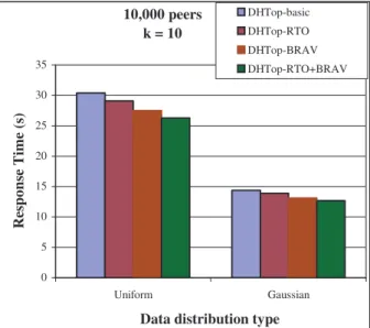
5.5 Effect of Data Distribution

In this section, we investigate the response time of our algorithm over two Uniform and Guassian data sets that we have generated synthetically, as described in Section 5.1.

Using our simulator, Figure 9 shows the response time of our four algorithms over Uniform and Guassian data sets, with the other parameters set as in Table 1 and 2. The response time of all four algorithms over the Guassian data set is much better than their response time over the Uniform data set. The reason stems from that, in the Guassian distribution, a high percentage of generated values are around the mean value and a very small percentage of the values are in the extremes, i.e. more than 95% of generated values are between λ-2δ and λ+2δ

where λ is the mean value and δ is the standard

deviation. This characteristic of the Guassian distribution makes the end condition of DHTop hold sooner over the Guassian data set than over the Uniform data set.

Figure 9. Response time over uniform and Guassian

data sets

5.6 Effect of Batch Retrieval of Attribute Values

In this section, we study the effect of the number of retrieved attribute values per message on the BRAV optimization. In the previous tests, this number was 10. In this section, we vary this number and study its effect on response time.

Using our simulator, Figure 10 shows the response time of DHTop-BRAV while increasing the number of attribute values retrieved per message, and the other parameters

10,000 peers k = 10 0 5 10 15 20 25 30 35 Uniform Gaussian

Data distribution type

R es po ns e T im e (s ) DHTop-basic DHTop-RTO DHTop-BRAV DHTop-RTO+BRAV

set as in Table 1 and Table 2. The best response time is for the case where peers send all their stored values to pint. In our tests, the number of attribute values, which are stored at each peer, is not very high. Should this number be very high, having each peer send all its attribute values to

pint would cause useless values to be sent, as the algorithm would end before using them. In this case, to avoid wasting network bandwidth, it is better to send in each message only a part of the attribute values, e.g. at most 10*k attribute values per message.

10,000 peers k = 10 25 26 27 28 29 30 31 32 33 34 1 5 9 13 17 all values

Number of attribute values per message

R es po ns e T im e (s ) DHTop-BRAV

Figure 10. Response time vs. number of attribute

values sent per message

6.

Related Work

Efficient processing of top-k queries is both an important and hard problem that has received recently much attention. The most efficient algorithms are based on the TA algorithm [14][16][24]. We have briefly introduced the TA algorithm in Section 1, initially designed for centralized systems.

Several TA-style algorithms have been proposed for distributed systems. The first distributed TA-style algorithm has been proposed in [8] with the objective of processing top-k queries over Internet data sources for recommendation services (e.g. restaurant ratings). In [9], the authors propose a TA-style algorithm to answer top-k queries in distributed systems. The algorithm reduces the communication cost by pruning away ineligible data items and restricting the number of round-trip messages between the query initiator and the other peers. In [23], an approximate TA-style algorithm is proposed for wide-area distributed systems. It uses the concept of bloom filters for

reducing the data communicated over the network upon processing top-k queries, and yields significant performance benefits with small penalties in result precision.

Overall, these TA-style algorithms have focused on reducing data communication in traditional distributed systems, not P2P systems. Top-k query processing in P2P systems has therefore started to attract attention. In [6], the authors address top-k query processing in Edutella, a super-peer network in which a small percentage of nodes are super-peers and are assumed to be highly available with very good computing capacity. The algorithm is not TA-style. It proceeds by sending the query to the super-peers and via them to ordinary peers, and finally collecting top answers by the super-peers. The authors also develop efficient routing methods among super-peers in a hypercube topology. However, the algorithm cannot apply to DHTs where data storage is based on keys.

In [1][2], we proposed a (non TA-style) algorithm for top-k query processing in unstructured P2P systems. The algorithm proceeds by flooding the query to the peers that are in a limited distance from the query initiator. And the top-k answers are gathered in a tree-based fashion by intermediate peers. We proposed efficient methods for reducing the communication cost of query execution in unstructured P2P systems. However, in the current paper our focus is on supporting top-k query processing in DHTs where data storage and retrieval is based on keys.

7.

Conclusion

In this paper, we addressed the problem of top-k query processing in Distributed Hash Tables (DHTs). We first proposed a mechanism for data storage in DHTs which provides good support for exact-match queries and enables efficient execution of our top-k query processing algorithm. Then, we proposed an efficient TA-style algorithm for top-k query processing in DHTs. Although, our algorithm is TA-style, it is much more general since it supports a large set of non monotone scoring functions including linear functions. In fact, it is the first TA-style algorithm that supports linear scoring functions. We proved analytically the correctness of our algorithm.

We validated our algorithm through implementation and experimentation over a

64-node cluster and evaluated its scalability through simulation up to 10,000 peers using SimJava. We studied the effect of several parameters (e.g. number of peers, k, number of attribute’s sub-domains, etc.) on the performance of our base algorithm and its optimizations. The results show very good performance, in terms of communication cost and response time. The response time and communication cost of our algorithm grow logarithmically with the number of peers of the DHT. Increasing the number of top tuples requested, i.e. k, increases very slightly the response time of our algorithm. In addition, increasing the number of attributes’ sub-domains (to increase load balancing) has very little impact on the response time and communication cost of individual queries. Finally, our two simple optimizing strategies (batch retrieval of attribute values and retrieving each tuple at most once) can reduce response time by up to 20%. In summary, this demonstrates that top-k queries, an important kind of complex queries, can now be efficiently supported in DHTs.

References

[1] Akbarinia, R., Pacitti, E., and Valduriez, P. Reducing Network Traffic in Unstructured P2P Systems Using Top-k Queries. J.

Distributed and Parallel Databases, 2006 (to

appear).

[2] Akbarinia, R., Martins, V., Pacitti, E., and Valduriez, P. Top-k Query Processing in the APPA P2P System. Int. Conf. on High

Performance Computing for Computational Science (VecPar), 2006.

[3] Akbarinia, R., Martins, V., Pacitti, E., and Valduriez, P. Design and Implementation of Atlas P2P Architecture. Global Data

Management (Eds. R. Baldoni, G. Cortese,

F. Davide), IOS Press, 2006.

[4] Akbarinia, R. and Martins, V. Data Management in the APPA P2P System. Int.

Workshop on High-Performance Data

Management in Grid Environments

(HPDGrid), 2006.

[5] Babcock, B., and Olston, C. Distributed Top-K Monitoring. SIGMOD Conf., 2003. [6] Balke, W.-T., Nejdl, W., Siberski, W., and

Thaden, U. Progressive Distributed Top k Retrieval in Peer-to-Peer Networks. ICDE

Conf., 2005.

[7] Böhm, C., Berchtold, S., and Keim, D.A. Searching in high-dimensional spaces: Index structures for improving the performance of multimedia databases. ACM Computing

Surveys 33(3), 2001.

[8] Bruno, N., Gravano, L., and Marian, A. Evaluating Top-k Queries over Web-Accessible Databases. ICDE Conf., 2002. [9] Cao, P., Wang, Z. Efficient Top-K Query

Calculation in Distributed Networks. PODC

Conf., 2004.

[10] Chaudhuri, S., Gravano, L., and Marian, A. Optimizing Top-K Selection Queries over Multimedia Repositories, J. IEEE Transactions on Knowledge and Data Engineering 16(8), 2004.

[11] Ciaccia, P., and Patella, M. Searching in metric spaces with user-defined and approximate distances. J. ACM Transactions

on Database Systems (TODS), 27(4), 2002.

[12] Dabek, F., Zhao, B.Y., Druschel, P., Kubiatowicz, J., and Stoica, I. Towards a Common API for Structured Peer-to-Peer Overlays. Proc. of Int. Workshop on

Peer-to-Peer Systems (IPTPS), 2003.

[13] DeVries, A.P., Mamoulis, N., Nes, N., and Kersten, M.L. Efficient k-NN Search on Vertically Decomposed Data. SIGMOD

Conf., 2002.

[14] Fagin, R., Lotem, J., and Naor, M. Optimal aggregation algorithms for middleware. J. of

Computer and System Sciences 66(4), 2003.

[15] Gao, J., and Steenkiste, P. An Adaptive Protocol for Efficient Support of Range Queries in DHT-Based Systems. IEEE Int.

Conf. on Network Protocols (ICNP), 2004.

[16] Güntzer, U., Kießling, W., and Balke, W.-T. Optimizing Multi-Feature Queries for Image Databases. VLDB Conf., 2000.

[17] Harren, M. et al. Complex Queries in DHT-based Peer-to-Peer Networks. Proc. of

Int. Workshop on Peer-to-Peer Systems (IPTPS), 2002.

[18] Hjaltason, G.R., and Samet, H. Index-driven similarity search in metric spaces. J.

ACM Transactions on Database Systems (TODS), 28(4), 2003.

[19] Howell, F., and McNab, R. SimJava: a Discrete Event Simulation Package for Java with Applications in Computer Systems Modeling. Proc. of Int. Conf. on Web-based

[20] Huebsch, R., Hellerstein, J., Lanham, N., Thau Loo, B., Shenker, S., and Stoica, I. Querying the Internet with PIER. VLDB

Conf., 2003.

[21] Koudas, N., Ooi, B.C., Tan, K.L., and Zhang, R. Approximate NN queries on Streams with Guaranteed Error/performance Bounds. VLDB Conf., 2004.

[22] Long, X., and Suel, T. Optimized Query Execution in Large Search Engines with Global Page Ordering. VLDB Conf., 2003. [23] Michel, S., Triantafillou, P., and Weikum,

G. KLEE: A Framework for Distributed Top-k Query Algorithms. VLDB Conf., 2005.

[24] Nepal, S., and Ramakrishna, M.V. Query Processing Issues in Image (Multimedia) Databases. ICDE Conf., 1999.

[25] Persin, M., Zobel, J., and Sacks-Davis, R. Filtered Document Retrieval with Frequency-Sorted Indexes, J. of the

American Society for Information Science (JASIS), 47(10), 1996.

[26] Ratnasamy, S., Francis, P., Handley, M., Karp, R.M., and Shenker, S. A scalable content-addressable network. Proc. of

SIGCOMM, 2001.

[27] Ratnasamy, S., Stoica, I., and Shenker, S. Routing Algorithms for DHTs: Some Open Questions. Proc. of Int. Workshop on

Peer-to-Peer Systems (IPTPS), 2002.

[28] Rowstron, A. I.T., and Druschel, P. Pastry: Scalable, Decentralized Object Location, and Routing for Large-Scale Peer-to-Peer Systems. Proc. of ACM Int. Conf. on

Distributed Systems Platforms (Middleware),

2001.

[29] Saroiu, S., Gummadi, P.K., and Gribble, S.D. A Measurement Study of Peer-to-Peer File Sharing Systems. Proc. of Multimedia

Computing and Networking (MMCN), 2002.

[30] Soffer, A., Carmel, D., Cohen, D., Fagin, R., Farchi, E., Herscovici, M., and Maarek, Y.S. Static Index Pruning for Information Retrieval Systems. SIGIR Conf., 2001. [31] Stoica, I., Morris, R., Karger, D.R.,

Kaashoek, M.F., and Balakrishnan, H. Chord: A scalable peer-to-peer lookup service for internet applications. Proc. of

SIGCOMM, 2001.

[32] Williams, S.A., Press, H., Flannery, B.P., and Vetterling, W.T. Numerical Recipes in

C: The Art of Scientific Computing.

Cambridge Univ. Press, 1993.

[33] Zhao, B.Y., Kubiatowicz, J., and Joseph, A.D. Tapestry: a Fault-tolerant Wide-Area Application Infrastructure. Computer Communication Review 32(1), 2002.