Comparison of two-dimensional flood propagation models: SRH-2D and Hydro_AS-2D

Titre:

:

Comparison of two-dimensional flood propagation models: SRH-2D

and Hydro_AS-2D

Auteurs:

Authors

: Basile Lavoie et Tew-Fik Mahdi

Date: 2017

Type:

Référence:

Citation

:

Lavoie, B. & Mahdi, T.-F. (2017). Comparison of two-dimensional flood propagation models: SRH-2D and Hydro_AS-2D. Natural Hazards, 86(3), p. 1207-1222. doi:10.1007/s11069-016-2737-7

Document en libre accès dans PolyPublie

URL de PolyPublie:

PolyPublie URL: https://publications.polymtl.ca/2999/

Version: Version finale avant publication / Accepted version_{Révisé par les pairs / Refereed} Conditions d’utilisation:

Terms of Use: Tous droits réservés / All rights reserved Document publié chez l’éditeur officiel

Document issued by the official publisher

Titre de la revue:

Journal Title: Natural Hazards (vol. 86, no 3)

Maison d’édition:

Publisher: Springer

URL officiel:

Official URL: https://doi.org/10.1007/s11069-016-2737-7

Mention légale:

Legal notice:

This is a post-peer-review, pre-copyedit version of an article published in Natural

Hazards. The final authenticated version is available online at: https://doi.org/10.1007/s11069-016-2737-7

Ce fichier a été téléchargé à partir de PolyPublie, le dépôt institutionnel de Polytechnique Montréal

This file has been downloaded from PolyPublie, the institutional repository of Polytechnique Montréal

1

-

-1

Basile Lavoie1_{, Tew-Fik Mahdi Ph.D.}2

3

1_{Département des génies Civil, Géologique et des Mines (CGM), École Polytechnique de}

4

Montréal, C.P. 6079, succursale Centre-Ville, Montréal, QC H3C 3A7, Canada. Email: 5

[email protected] 6

2 _{Professor, Département des génies Civil, Géologique et des Mines (CGM), École Polytechnique}

7

de Montréal, C.P. 6079, succursale Centre-Ville, Montréal, QC H3C 3A7, Canada (Corresponding 8

author). Email: [email protected]. Phone: (514) 4711 Ext.: 5874. Fax: (514) 340-9

4191 10

11

This article presents a comparison between two two-dimensional finite volume flood 12

propagation models: SRH-2D and Hydro_AS-2D. The models are compared using an 13

experimental dam-break test-case provided by Soares-Frazão (2007). Four progressively refined 14

meshes are used, and both models react adequately to mesh and time step refinement. 15

Hydro_AS-2D shows some unphysical oscillations with the finest mesh and a certain loss of 16

accuracy. For that test-case, Hydro_AS-2D is more accurate for all meshes and generally faster 17

than SRH-2D. Hydro_AS-2D reacts well to automatic calibration with PEST, whereas SRH-2D has 18

some difficulties in retrieving 19

Model comparison; Two-dimensional flow modeling; Hydro_AS-2D; 20

SRH-2D; Automatic calibration 21

2 D Hydraulic diameter 23 e Source term 24 g Gravitational acceleration 25 h Water depth 26

k Turbulent kinetic energy 27 n 28 Sfx, Sfy Energy slope 29 Sbx, Sby Bed slope 30 T Turbulence stress 31 u, v Velocity components 32

z Water surface elevation 33

zb Bed elevation

34

Eddy viscosity 35

0 Kinematic viscosity of water

36

t Turbulent eddy viscosity

37 Mass density 38 Shear stress 39

1 Introduction

Flood propagation may induce important human and material losses and remains a major 41

challenge for hydraulic engineers due to the complexity of the phenomenon and therefore to 42

the difficulties that arise in their numerical modeling. Two-dimensional models are now widely 43

used in flood propagation modeling owing to the gain in precision they offer and their relatively 44

small time consumption. Different types of methods were used for the numerical modeling of 45

shallow water equations as finite differences, finite elements and finite volumes. For fluid flows, 46

the last is currently accepted as the most accurate and has been implemented in several models 47

such as TUFLOW-FV (BMTWBM 2014), RiverFlow2D (Hydronia 2015), SRH-2D (Lai 2008), 48

Hydro_AS-2D (Nujic 2003), HEC-RAS (Brunner 2016) and BASEMENT (Vetsch 2015). If these 49

models are usually validated by their designer, few model-to-model comparisons exist. It is yet 50

of great importance for practicing engineers to have objective and precise comparisons on 51

which they can rely for the choice of a flood propagation model. The aim of this paper is to 52

provide such a comparison for two models: Hydro_AS-2D, which is mainly used in European 53

countries, and SRH-2D, largely used in North America. 54

3 SRH-2D was validated against numerous experimental, analytical and river cases. Lai (2008) and 55

Lai (2010) showed that the model reacts correctly compared with the analytical solution of a 56

transcritical flow with a hydraulic jump in a 1D channel that was proposed by MacDonald (1996). 57

SRH-2D was also used to model the 2D diversion flow case measured by Shettar et Murthy 58

(1996) with the conclusion that the flow was better modeled along the walls by SRH-2D with the 59

k-epsilon turbulence model than with the parabolic model (Lai 2008; Lai 2010). Experimental 60

data of a channel with bend proposed by Zarrati et al. (2005) were modeled with SRH-2D and 61

showed that the computed water depth was less sensitive to mesh resolution than the velocity 62

(Lai 2008; Lai 2010). The model was used to evaluate the impact of a dam removal on the Sandy 63

River Delta with satisfactory results. A similar study was undertaken for the Savage Rapids dam 64

removal and achieved good results in modeling the water depth and hydraulic jump (Lai 2008; 65

Lai 2010). 66

Jones (2011) made a comparison of four two-dimensional hydrodynamic models: ADH (Berger et 67

al. 2013), FESWMS (Froehlich 2002), RMA2 (Donnell 2006) and Hydro_AS-2D (Nujic 2003). 68

Applied to three test-cases, Hydro_AS-2D proved to be the most stable and easy to use and was 69

able to run in some cases where other models could not. Hydro_AS_2D was also the fastest 70

model. 71

Tolossa (2008) and Tolossa et al. (2009) compared the two-dimensional hydrodynamic models 72

Hydro_AS-2D and SRH-W, which was the first released version of SRH-2D. The models were 73

compared on three river reaches and were able to appropriately recreate the water depth. The 74

authors report that SRH-W seems more sensitive to mesh refinement, meaning that a finer 75

mesh was needed to reach a precision comparable to Hydro_AS-2D. SRH-W was the fastest 76

model of this study. 77

4 Both models have been tested in numerous studies and have been proven to be reliable. 78

However, the previous comparisons and test-cases did not state which of SRH-2D and 79

Hydro_AS-2D could best predict the water depth. It is therefore the purpose of this paper to 80

provide a clear statement on which model is best for forecasting flow parameters. The 81

computation time will be compared as well to confirm or nuance previous studies. In addition, a 82

new feature, which has, to the best of our knowledge, never been used to compare 83

hydrodynamic models, is studied for the purpose of this comparison: automatic calibration. 84

Automatic calibration is becoming increasingly used in hydrodynamic and hydrologic modeling 85

(Ellis et al. 2009; Fabio et al. 2010; McCloskey et al. 2011; McKibbon et Mahdi 2010) because it 86 87 rrectly to an automatic 88 calibration. 89

2 Presentation of Models

2.1 SRH-2D Version 3

SRH-2D solves the shallow water equations using the following form (Lai 2008; Lai 2010): 92 (Eq. 1) 93 (Eq. 2) 94 (Eq.3) 95

The friction is determined using the Manning equation: 96

5 (Eqs. 4 and 5)

97

Boussinesq equations are used to compute the turbulence stresses: 98 (Eq. 6) 99 (Eq. 7) 100 (Eq. 8) 101

where h is the water depth, u and v are the velocity components, z is the water surface 102

shear stress, g is the 103 0 t is the 104 105 coefficient. 106

SRH-2D proposes two turbulence models: k-epsilon and depth-averaged parabolic models. The 107

parabolic model is used in the present study because it is the only turbulence model used by 108

Hydro_AS-2D, and a proper comparison necessitates identical parameters. SRH-2D uses a 109

wetting drying front limit of 0.001 m. Below this value, water depth is considered to be equal to 110

0 m on the cell, and SRH-2D does not solve the shallow water equations (Lai 2010). 111

2.2 Hydro_AS-2D Version 4

Shallow water equations, as solved by Hydro_AS-2D, are expressed in vectors (Nujic 2003): 113

(Eq. 9) 114

6 (Eq. 10)

115

(Eq. 11) 116

The bed slope is defined as follows: 117

(Eqs. 12 and 13) 118

The energy slope is computed following the Darcy Weisbach equation, and the friction 119

coefficient is determined with the Manning formula: 120

(Eq. 14) 121

f is the energy slope, zb is the bed elevation, and D is the

122

hydraulic diameter. 123

The default wetting drying front limit is set to 0.01 m but is lowered to 0.001 m for the current 124

study. Time steps are calculated automatically and continuously by Hydro_AS-2D over the 125

modeling. 126

2.3 SMS Version 12.1

The Surface water Modeling System, SMS (AQUAVEO 2016), facilitates the required 128

pretreatment and post-treatment for hydraulic modeling of open channel flow. SMS includes 129

many characteristics of GIS software and uses them, for example, in the creation of quality 130

meshes. The results may be viewed in three dimensions, and many tools are available for their 131

7 treatment, which makes SMS very versatile and usable with multiple models (AQUAVEO 2016). 132

For the present study, SMS allows with great ease the use of the same mesh and boundary 133

conditions for the two models, SRH-2D and Hydro_AS-2D, which is necessary for a proper 134

comparison. 135

2.4 PEST Version 13

PEST (Doherty 2005) is a software program that executes the automatic calibration and 137

sensibility analysis of any model based on input and output files. In this study, only the 138

automatic calibration module is used. Automatic calibration with PEST requires three main types 139

of files: template, instruction and control files (figure 1). 140

o Template files act as models for PEST when creating input files to calibrate the model 141

(i.e., SRH-2D and Hydro_AS-2D). 142

o Instruction files aid the

143

values that should be used for the calibration. 144

o The control file contains calibration instructions, such as stopping criteria and observed 145

values. It 146

refer. 147

PEST is therefore model independent and relatively simple to use, which makes it a powerful 148

tool for the calibration of two-dimensional hydrodynamic models. 149

3 Methodology

The comparison of SRH-2D and Hydro_AS-2D is made on experimental data and aims to verify 151

the accuracy of both models, their sensitivity to spatial and time discretization, and their 152

response to automatic calibration. 153

8

3.1 Test-case

154

The two models are compared using an experimental dataset presented by Soares-Frazão (2007) 155

in which a dam break wave over a triangular bottom sill is studied. The rectangular channel has 156

a width of 0.5 m and a length of 5.6 m, and the sill height is 0.065 m with a symmetrical slope of 157

1/3_.

158

The initial conditions (figure 2) are made of an upstream reservoir in which the water depth is 159

0.111 m and by a downstream pool, isolated from the rest of the channel by the sill, with a 160

water depth of 0.02 m. The central section is initially dry. The reservoir is isolated by a gate 161

whose sudden removal creates the propagation of the dam-break wave upon the channel. 162

All four boundaries of the channel consist of walls, meaning that the wave will successively 163

reflect against the downstream and upstream walls. The wave first propagates on the dry bed to 164

reach the sill where the water is partly reflected to the upstream part of the channel and partly 165

continues to reach the water pool located downstream of the sill. Reflections are then 166

simultaneously observed in the sections of the channel located on both sides of the sill. 167

Three gauges are positioned around the triangular sill to monitor the incidence of this feature 168

on the flow. The monitoring lasts 45 s, during which the water depths are available every 0.01 s, 169

for a total of 4501 measurements for each gauge. 170

3.2 Time Step and Mesh Sensitivity and Water Depth Accuracy

The simulation is made with SRH-2D on four progressively refined meshes (figure 3) that are all 172

modeled with five time steps (tables 1 and 2). These twenty simulations are then used to 173

investigate the sensitivity of SRH-2D to these parameters and will ensure that a mesh and time 174

step independent solution is achieved. The time step providing the best results is afterward 175

used for the comparison with Hydro_AS-2D. Hydro_AS-2D computes the time step required to 176

9 fulfill the Courant condition, so the user does not have influence on that parameter. Therefore, 177

only the mesh sensitivity is evaluated for this model. The meshes used are the same as those 178

presented above for SRH-2D. 179

The comparison is then made on the four meshes, and the quality of the simulations is 180

quantified through the calculation of the root mean squared error (RMSE) considering the 181

calculated and measured water depth every 0.1 s for a total of 450 benchmark measurements 182

by gauge. 183

All simulations last 45 s, and the depth-averaged parabolic model is used for turbulence for both 184

SRH-2D and Hydro_AS-2D. The minimum water depth for the treatment of the wetting and 185

drying front is 0.001 m, and the maximum velocity is 15 m/s for Hydro_AS-2D. The wetting and 186

drying front limit is also 0.001 m for SRH-2D, but the maximum velocity is unknown. All wall 187

boundaries are assigned a no-slip condition. All calculations are made with a 64 GB server with 188

an Intel Xeon CPU E5-2630 v3 @2.40 GHz processor. 189

3.3 Response to Automatic Calibration

The dam-break models, using SRH-2D and Hydro_AS-2D, are automatically calibrated with PEST 191

192

Soares-Frazão (2007) and the incidence of that calibration on the water depth RMSE. 193

The automatic calibration requires experimental measurements to compare the simulations and 194

195

the number of measurements, all available measurements cannot be used. The number of 196

benchmark values is therefore set to 27, meaning one measurement at each gauge every 5 s. 197

198

vary between 0.005 s/m1/3 _{and 0.05 s/m}1/3 _{for both SRH-2D and Hydro_AS-2D.}

10

4 Results and Discussion

200

4.1 Time Step and Mesh Sensitivity SRH-2D

Figure 4 presents the evolution of RMSE relative to time step refinement for each gauge and 202

each mesh and shows a quick stabilization of the RMSE for the coarsest mesh, whereas the 203

finest mesh has a drastic reduction of its error between the first and fourth time steps (ex: from 204

0.0182 m to 0.0092 m for gauge 3). The error is insignificantly modified between the fourth and 205

fifth time steps (from 0.0092 m to 0.0087 m for gauge 3); these solutions can then be 206

considered to have reached time step independence. 207

The fifth time step gives the best solution for all meshes. It is used to compute the evolution of 208

water depth RMSE relative to mesh refinement, which can be observed in figure 5, and 209

diminishes with the mesh density (from 0.0094 m to 0.0087 m for gauge 3). 210

These results conform to theory because the time step needed to ensure stability, and 211

convergence is reduced proportionally to the grid size. SRH-2D has a good response to time step 212

and mesh density refinement. 213

4.2 Mesh Sensitivity Hydro_AS-2D

Hydro_AS-2D continuously adjusts the time step during the simulation to ensure numerical 215

stability. Therefore, only the mesh sensitivity is addressed. Figure 6 shows a global reduction of 216

RMSE following the mesh refinement with the exception of gauges 1 and 3, which present a 217

slight increase for the fourth mesh (0.0004 m for gauge 1 and 0.0001 m for gauge 3). Similar 218

results were published by and Boz et al. (2014), who respectively 219

investigated the influence of mesh density on the resolution of shallow water equations with 220

11 the Q-scheme and the MUSCL Hancock scheme and on the resolution of the Navier Stokes 221

equations with the CFD code ANSYS CFX. 222

4.3 Water Depth Profiles and Oscillations

Figure 7 shows the evolution of water depth in time for all meshes at gauge 1 as calculated by 224

Hydro_AS-2D. The mesh refinement greatly benefits the results for the first 15 s of the 225

simulation where the experimental and computed water depths become very similar. However, 226

the refinement seems to increase the oscillation amplitude beyond the 15th _{second. These}

227

oscillations are not physically representative when compared to the experimental line. This 228

phenomenon may also be noted at a smaller scale for gauge 2 but is absent at gauge 3, which 229

may be because these oscillations are induced by the wall reflection. This phenomenon was also 230

noted by , who observed that the oscillation amplitude was increasing with 231

increasing mesh refinement but observed no dependence between the oscillation frequency 232

and the mesh density, which is not the case of the current study in which lower spatial 233

resolution seems to yield a higher oscillation frequency (figure 7). 234

SRH-2D has its general water depth results greatly improved by the mesh refinement, whereas 235

the experimental and computed depths become closer (figure 8). The augmented spatial 236

resolution also gives a better representation of the oscillations. Moreover, these oscillations are 237

offset in time but stay physically consistent with the experimental data unlike Hydro_AS-2D. 238

Comparing figures 7 and 8, Hydro_AS-2D seems to provide a better fit with the experimental 239

data for all meshes, especially for the first 15 s. 240

12

4.4 Water Depth RMSE

241

Figure 9 shows a comparison of computed water depth RMSEs for SRH-2D and Hydro_AS-2D 242

with all four meshes. The smallest time step is used for all SRH-2D simulations because it 243

provides the best results. For all meshes, Hydro_AS-2D is more accurate at all gauges and all 244

erved at the 245

third gauge (0.0094 m for SRH-2D versus 0.0038 m for Hydro_AS-2D with the coarsest mesh). 246

SRH-2D has its largest error at gauge 3, which is initially dry and may represent the difficulty of 247

modeling the wave propagation on a dry bed. This was noted as a current difficulty in numerical 248

modeling by Soares-Frazão (2007) and was one of the main purposes of the experiment used in 249

the current study. Hydro_AS-2D shows the most important error at gauge 2, which is placed 250

after the downstream side of the sill. This may be because the important slope of the sill creates 251

a flow that is not fully 2D and is therefore more difficult to represent by the model. 252

4.5 Computation time

Computation time is highly related to the number of mesh elements and time steps. Only mesh 254

density influence is studied for Hydro_AS-2D because the model automatically adjusts the time 255

step. SRH-2D gives full control of these two parameters, so both mesh density and time step 256

sensitivity are considered. 257

Figure 10 shows the evolution of computation time relative to the time step of all meshes for 258

SRH-2D. The computation time increases with increasing mesh and time step resolutions. There 259

is a dramatic increase in the computational time for time step 5 (0.0001 s) compared with time 260

step 4 (0.0004 s), especially for the finest mesh (11.6 h versus 39.1 h). 261

Because the time step has such a drastic influence on the computation time, this parameter 262

must be properly chosen to form a reliable comparison and avoid the use of a very small time 263

13 step that would unnecessarily increase the computation time. Therefore, the chosen time step 264

for SRH-2D is the one allowing time step independence of the model and is selected based on 265

the results of figure 4 (section Time Step and Mesh Sensitivity). Table 3 summarizes the time 266

step used for the two models in the computation time comparison. The computation times are 267

pretty much equal for the first mesh, but Hydro_AS-2D is generally faster by an average factor of 268

7.51 h/h (figure 11). One should note that the largest difference is observed for the finest mesh 269

where Hydro_AS-2D is 15.8 times faster, whereas the time step is almost the same for both 270

SRH-2D HYDRO_AS-2D=0.00037 s). The capacity of Hydro_AS-2D to

271

parallelize the calculation can explain this difference between the two models. The code 272

structures may also impact the computation time, but this information is not available for these 273

models. 274

4.6 Response to Calibration

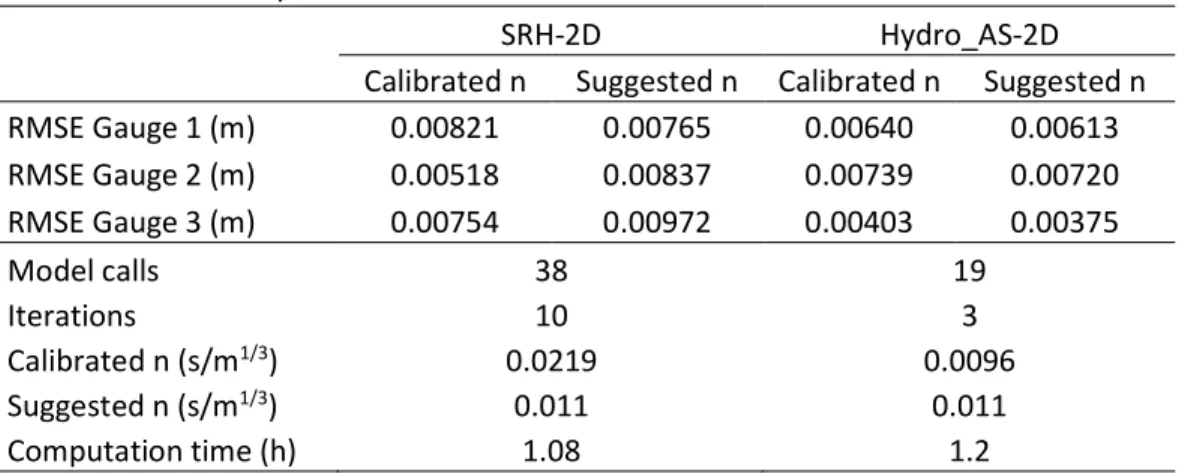
Table 4 summarizes the results and parameters of the automatic calibrations with PEST for the 276

two models. SRH-2D necessitates 10 iterations and 38 model calls, whereas Hydro_AS-2D 277

completes the calibration in 3 iterations and 19 model calls. SRH-2D is slightly faster (1.08 h 278

versus 1.2 h), which is not surprising considering that this model has been shown to be faster for 279

the coarsest mesh, the only mesh used for the automatic calibration, when used with a time 280

step of 0.005 s (see section Computation Time). 281

Automatic calibration with Hydro_AS-282

s/m1/3_{, which is very similar to 0.011 s/m}1/3 _{as suggested by Soares-Frazão (2007). SRH-2D, when}

283

calibrated, gives a very different value of 0.0219 s/m1/3_{. Hydro_AS-2D provides very similar}

284

; the maximal difference 285

is 0.0003 m, which is observed at gauge 3. This is consistent with the fact that the calibrated 286

14 -2D has a 287

good response to automatic calibration. When calibrated, SRH-2D shows a greater improvement 288

of its RMSE, which decreases by up to 0.0032 m at gauge 2. If only the water depth RMSE is 289

considered to qualify the automatic calibration, SRH-2D seems to be benefiting from a 290

ent that is approximatively twice the suggested coefficient. This is 291

unlikely because that parameter would lose its physical representativeness of the actual 292

293

time at gauge 1 (figure 12). The calibrated computed water depth becomes closer to the 294

experimental water depth in the second half of the experiment; however, it is clear that the 295

shape of oscillation is lost with the calibration and is better represented by the original 296

297

calibration is unsuitable for SRH-2D in that case. One can note that Hydro_AS-2D remains 298

generally more accurate than SRH-2D, the only exception being gauge 2 at which SRH-2D gives a 299

smaller RMSE. 300

5 Conclusion

Two flood propagation models, Hydro_AS-2D and SRH-2D, were compared in terms of their 302

capacity to properly model an experimental dam-break test case. The two models were shown 303

to have a good response to mesh and time step refinement; however, Hydro_AS-2D showed 304

unphysical oscillations and an increase in the water depth RMSE at two of the three gauges with 305

the finest mesh. These observations support the idea that too much spatial resolution could 306

negatively affect the accuracy of a model as noted by and Boz et al. (2014). 307

Hydro_AS-2D computed lower RMSEs for all meshes and was therefore more accurate than 308

SRH-2D. Hydro_AS-2D was up to 15.8 times faster than SRH-2D. This contrasts with the results 309

15 of Tolossa (2008) and Tolossa et al. (2009), who found that W (the previous version of SRH-310

2D) was faster than Hydro_AS-2D. Hydro_AS-2D responded well to the automatic calibration of 311

312

whereas SRH-2D computed a very different coefficient that lowered the water depth RMSE but 313

with no physical representativeness of the actual channel. 314

This research has exposed some of the differences between two major hydrodynamic models 315

and clarified their respective assets to offer an objective point of comparison that will be helpful 316

for industrial and research engineers in choosing a modeling tool for flood propagation. 317

318

This research was supported in part by a National Science and Engineering Research Council 319

(NSERC) Discovery Grant, application No: RGPIN-2016-06413. 320

321

AQUAVEO (2016). "SMS 12.1 - The Complete Surface-water Solution." 322

< http://www.aquaveo.com/software/sms-surface-water-modeling-system-323

introduction>. (March 10, 2016). 324

Berger, R. C., Tate, J. N., Brown, G. L., et Savant, G. (2013). "Adaptive Hydraulics Users Manual." 325

Coastal and Hydraulics Laboratory Engineer Research and Development Center, 99. 326

BMTWBM (2014). "TUFLOW FV User Manual." Flexible Mesh Modelling, BMT WBM, Brisbane, 327

Australia, 183. 328

Boz, Z., Erdogdu, F., et Tutar, M. (2014). "Effects of mesh refinement, time step size and 329

numerical scheme on the computational modeling of temperature evolution during 330

natural-convection heating." Journal of Food Engineering, 8-16. 331

Brunner, G. W. (2016). "HEC-RAS River Analysis System User's Manual." US Army Corps of 332

Engineers, Davis, CA, USA, 960. 333

Doherty (2005). "PEST, Model-Independant Parameter Estimation, USer Manual: 5th Edition." 334

Watermark Numerical Computing. 335

Donnell, B. P. (2006). "RMA2 WES Version 4.5." I. King, J. V. Letter, W. H. McAnally, et W. A. 336

Thomas, eds., US Army, Engineer Research and Development Center, 277. 337

-338

Spatial Resolution for Two-Dimensional Shallow-Water Model Accuracy." Journal of 339

Hydraulic Engineering, 917-925. 340

Ellis, R. J. l., Doherty, J., Searle, R. D., et Moodie, K. (2009). "Applying PEST (Parameter 341

ESTimation) to improve parameter estimation and uncertainty analysis in WaterCAST 342

16 models." 18th World IMACS/MODSIM Congress, Modelling and Simulation Society of 343

Australia and New-Zealand Inc., 3158-3164. 344

Fabio, P., Aronica, G. T., et Apel, H. (2010). "Towards automatic calibration of 2-D flood 345

propagation models." Hydrology and Earth System Sciences, 10.5194/hess-14-911-2010, 346

911-924. 347

Froehlich, D. C. (2002). "User's Manual for FESWMS FST2DH." Federal Highway Administration, 348

209. 349

Hydronia (2015). "RiverFlow2D Plus Two-Dimensional Finite-Volume River Dynamics Model." 350

Hydronia, Pembroke Pines, FL, USA, 157. 351

Jones, D. A. (2011). "The Transition from Earlier Hydrodynamic Models to Current Generation 352

Models." Master of Science, Brigham Young University, Brigham. 353

Lai, Y. G. (2008). "SRH-2D version 2: Theory and User's Manual." U.S. Department of the interior 354

- Bureau of Reclamation, Denver. 355

Lai, Y. G. (2010). "Two-Dimensional Depth-Averaged Flow Modeling with an Unstructured Hybrid 356

Mesh." Journal of Hydraulic Engineering, 12-23. 357

Lin, Z. (2010). "Getting Started with PEST." The University of Georgia, Athens, GA. 358

MacDonald, I. (1996). "Analysis and Computation of Steady Open Channel Flow." Doctor of 359

Philosophy, University of Reading, Reading, UK. 360

McCloskey, G. L. l. E., R.J., Waters, D. K., et Stewart, J. (2011). "PEST hydrology calibration 361

process for source catchments - applied to the Great Barrier Reef, Quennsland." 19th 362

International Congress on Modelling and Simulation, Modelling and Simulation Society 363

of Australia and New-Zealand Inc., 2359-2366. 364

McKibbon, J., et Mahdi, T.-F. (2010). "Automatic Calibration Tool for River Models Based on the 365

MHYSER Software." Natural Hazards, 54(3), 879-899. 366

Nujic, M. (2003). "Hydro_AS-2D A Two-Dimensional Flow Model For Water Mangement 367

Applications User's Manual."Rosenheim, Deutschland. 368

Shettar, A. S., et Murthy, K. K. (1996). "A numerical Study of Division of Flow in Open Channels." 369

Journal of Hydraulic Research, 34(5), 651-675. 370

Soares-Frazão, S. (2007). "Experiments of dam-break wave over a triangular bottom sill." Journal 371

of Hydraulic Research, 10.1080/00221686.2007.9521829, 19-26. 372

Tolossa, G. H. (2008). "Comparison of 2D Hydrodynamic models in River Reaches of Ecological 373

Importance:Hydro_AS-2D and SRH-W." Institut für Wasserbau, Universität Stuttgart, 374

Stuttgart. 375

Tolossa, H. G., Tuhtan, J., Schneider, M., et Wieprecht, S. "Comparison of 2D Hydrodynamic 376

Models in River Reaches of Ecological Importance Hydro_AS-2D and SRH-W." Proc., 33rd 377

IAHR World Congress, 604-611. 378

Vetsch, D. (2015). "System Manuls of Basement." Swiss Federal Institute of Technology Zurich, 379

Zurich, 178. 380

Zarrati, A. R., Tamai, N., et Jin, Y. C. (2005). "Mathematical Modeling of Meandering Channels 381

with a Generalized Depth Averaged Model." Journal of Hydraulic Engineering, 131(6), 382

467-475. 383

384 385

17

Figure Captions

386

Fig. 1. Automatic calibration with PEST Adapted from Lin (2010) 387

Fig. 2. Channel geometry, initial conditions and gauges positions 388

Fig. 3. Meshes (0.5 m × 0.45 m zone) 389

Fig. 4. Water depth RMSE relative to time step refinement at Gauges 1-3 SRH-2D 390

Fig. 5. Water depth RMSE relative to mesh refinement SRH-2D 391

Fig. 6. Water depth RMSE relative to mesh refinement Hydro_AS-2D 392

Fig. 7. Water depth at gauge 1 for meshes 1-4 Hydro_AS-2D 393

Fig. 8. Water depth at gauge 1 for meshes 1-4 SRH-2D 394

Fig. 9. Comparison of computed water depth RMSEs Meshes 1-4 395

Fig. 10. Computation time relative to time step refinement SRH-2D 396

Fig. 11. Comparison of computation time 397

Fig. 12. Comparison of 398

gauge 1 SRH-2D 399

18 400

Table 1. Time steps 401

Table 2. Meshes 402

Table 3. Time steps used for computation time comparison 403

Table 4. Calibration parameters and results

19 405

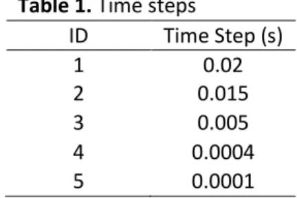
Table 1. Time steps ID Time Step (s) 1 0.02 2 0.015 3 0.005 4 0.0004 5 0.0001

Table 2. eshes ID Number of Cells 1 1 353 2 5 412 3 21 648 4 86 592

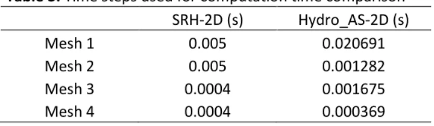
Table 3. Time steps used for computation time comparison SRH-2D (s) Hydro_AS-2D (s) Mesh 1 0.005 0.020691 Mesh 2 0.005 0.001282 Mesh 3 0.0004 0.001675 Mesh 4 0.0004 0.000369

Table 4. Calibration parameters and results

SRH-2D Hydro_AS-2D

Calibrated n Suggested n Calibrated n Suggested n

RMSE Gauge 1 (m) 0.00821 0.00765 0.00640 0.00613 RMSE Gauge 2 (m) 0.00518 0.00837 0.00739 0.00720 RMSE Gauge 3 (m) 0.00754 0.00972 0.00403 0.00375 Model calls 38 19 Iterations 10 3 Calibrated n (s/m1/3_{) 0.0219 0.0096} Suggested n (s/m1/3_{) 0.011 0.011} Computation time (h) 1.08 1.2