O
pen
A
rchive
T
OULOUSE
A
rchive
O
uverte (
OATAO
)
OATAO is an open access repository that collects the work of Toulouse researchers and
makes it freely available over the web where possible.
This is an author-deposited version published in :
http://oatao.univ-toulouse.fr/
Eprints ID : 14618
To link to this article : DOI:10.1063/1.4936980
URL :
http://dx.doi.org/10.1063/1.4936980
To cite this version : Lalanne, Benjamin and Abi Chebel, Nicolas and
Vejražka, Jiří and Tanguy, Sébastien and Masbernat, Olivier and Risso,
Frédéric Non-linear shape oscillations of rising drops and bubbles:
Experiments and simulations. (2015) Physics of Fluids, vol.27 (n°12).
pp.123305-1-123305-16. ISSN 1070-6631
Any correspondance concerning this service should be sent to the repository
administrator:
[email protected]
Non-linear shape oscillations of rising drops
and bubbles: Experiments and simulations
Benjamin Lalanne,1,2,3Nicolas Abi Chebel,1,2,3Jiří Vejražka,4
Sébastien Tanguy,1,3Olivier Masbernat,2,3and Frédéric Risso1,3
1Institut de Mécanique des Fluides de Toulouse, CNRS & Université de Toulouse, Toulouse, France
2Laboratoire de Génie Chimique, CNRS & Université de Toulouse, Toulouse, France 3Fédération de Recherche FERMAT, CNRS, Toulouse, France
4Institute of Chemical Process Fundamentals, Academy of Sciences of the Czech Republic, Prague, Czech Republic
This paper focuses on shape-oscillations of a gas bubble or a liquid drop rising in another liquid. The bubble/drop is initially attached to a capillary and is released by a sudden motion of that capillary, resulting in the rise of the bubble/drop along with the oscillations of its shape. Such experimental conditions make difficult the interpreta-tion of the oscillainterpreta-tion dynamics with regard to the standard linear theory of oscillainterpreta-tion because (i) amplitude of deformation is large enough to induce nonlinearities, (ii) the rising motion may be coupled with the oscillation dynamics, and (iii) clean conditions without residual surfactants may not be achieved. These differences with the theory are addressed by comparing experimental observation with numerical simulation. Simulations are carried out using Level-Set and Ghost-Fluid methods with clean interfaces. The effect of the rising motion is investigated by performing simulations under different gravity conditions. Using a decomposition of the bubble/drop shape into a series of spherical harmonics, experimental and numerical time evolutions of their amplitudes are compared. Due to large oscillation amplitude, non-linear couplings between the modes are evidenced from both experimental and numerical signals; modes of lower frequency influence modes of higher frequency, whereas the reverse is not observed. Nevertheless, the dominant frequency and overall damping rate of the first five modes are in good agreement with the linear theory. Effect of the rising motion on the oscillations is globally negligible, provided the mean shape of the oscillation remains close to a sphere. In the drop case, despite the residual interface contamination evidenced by a reduction in the terminal velocity, the oscillation dynamics is shown to be unaltered compared to that of a clean drop.
[http://dx.doi.org/10.1063/1.4936980]
I. INTRODUCTION
Interfacial dynamics plays a major role in dispersed two-phase flows since it governs the shape and motion of drops or bubbles. Shape oscillations involve eigenmodes characterized by their fre-quency and damping rate. These oscillation modes are excited by fluctuations of the surrounding flow. Depending on the time scales of these fluctuations relative to the characteristic time scales of interface dynamics, the shape may undergo large oscillations, which can either cause the breakup or just relax towards the equilibrium shape.1–3In this way, the interfacial dynamics also critically
affects the size distribution of bubbles or drops in multiphase flows.
The knowledge of bubble or drop eigenmodes is therefore a crucial issue for multiphase flows. They can be derived from the linearized Navier-Stokes equations when considering small oscillation amplitudes. The case of a drop oscillating around a spherical equilibrium shape in the absence of gravity is well known since the fundamental works of Miller and Scriven4and Prosperetti.5,6However,
in many practical situations, drop shape eigenmodes are modified by various physical mechanisms such as attachment to a support, action of surfactants, gravity, or drop motion. In the absence of gravity
and of imposed external flow, the cases of a drop constrained to a support7–10and of a free drop in the presence of surfactant11have been solved. Dealing theoretically with buoyancy and drop motion is
difficult owing to the coupling between the shape oscillations and the drop motion. Recently, the linear oscillations of a bubble or a drop rising in a liquid otherwise at rest have been investigated using direct numerical simulations.12For both bubbles and drops, the mode frequency is found to be a slightly
decreasing function of the Weber number based on the rising velocity. The damping rate for the drops and bubbles shows totally different trends. The damping rate of a drop is an increasing function of the Weber number, whereas the damping rate of a bubble is almost unaffected by the rising motion when it has reached its terminal shape and velocity. For millimeter-sized drops and bubbles rising at constant velocity within a liquid, the shape eigenmodes are weakly affected by the rising motion provided the Weber number based on terminal velocity is less than one.
We may question the relevance of these conclusions from numerical simulations for practical situations. Is it possible to produce experimental conditions in which they are valid? An experiment, in which a drop or a bubble undergoes axially symmetric damped oscillations, with conditions similar to those in computations, has been described in Ref.13. The drop is initially attached to the tip of a capil-lary. A sudden translation of the capillary brings about the drop detachment by causing a significant deformation of the interface. The drop then rises under the action of buoyancy and its shape oscillates. Two complications generally take place in experiments. The first arises from the fact that several modes are present simultaneously. Their amplitudes are difficult to control and usually exceed the linear limit, which is around 10% of the radius.12Second, the presence of surface-active contaminants can hardly be avoided, especially in the case of drops in another immiscible liquid.
The purpose of the present work is thus to investigate the moderate non-linear shape oscillations of a rising bubble (Sec.III) and a rising drop (Sec.IV) that appear in such an experimental device, by means of a detailed comparison of experimental observations with numerical simulations. In the numerical simulations, the same initial shape is prescribed as that measured in the experiments at the instant of detachment. Computations are also carried out for zero-gravity and high-gravity conditions. In the experiments, great care is taken to keep the fluids pure. For the bubble case, water remains pure enough so that the rising velocity is that of a clean bubble. For the drop case, some surface-active contaminants remain present. Owing to this variety of conditions, the comparison allows us to examine and disentangle the influence of both gravity and slight interface contamination on the oscillation dynamics.
II. PHYSICAL AND NUMERICAL EXPERIMENTS A. Experimental procedure
The experimental setup is the same as that used by Abi Chebel et al.13At a bottom of a vessel (11 × 11 cm in width and 26 cm height) filled with water, a bubble of air or a drop of heptane is injected through a glass capillary (250 µm in diameter). When the bubble/drop has reached the desired size, the capillary is rapidly moved vertically by the action of an electromagnetic coil, leading to its detachment. The motion of the capillary also induces relatively large, but axially symmetric initial deformation of the bubble/drop, due to which its shape oscillates during the free rise. The translation and the shape oscillations of the bubble/drop are recorded by a high-speed camera with a resolution of 5.9 µm/pixel for the drop and 6.8 µm/pixel for the bubble; the framing rate is 18 000 images per second. The position of the interface is detected in the recorded images by searching for gray level threshold, which is determined using Otsu’s method.14The interface
iden-tification includes also image interpolation, which increases the effective resolution of the detection of boundary location up to about one-fifth of a pixel size.
In the experiments, care is taken to ensure the purity of the system. Water is initially distilled and purified using a Watrex Ultrapur 40 system. Then, it is additionally cleaned within the exper-imental setup by circulating through a filter with activated-carbon cartridge in order to remove the residual surface-active contaminants. As we will show in Sections III andIV, this treatment is enough to ensure that the bubble interface is free of contaminants. However, for the heptane drop, measurements of terminal velocity indicate that the interface is still contaminated. The main source
TABLE I. Physical parameters of the experiment and the simulation.
Parameters R(mm) ρo(kg/m3) ρi(kg/m3) µo(Pa s) µi(Pa s) σ(N/m)
Bubble 0.388 998.3 1.226 1.02 × 10⁻³ 1.78 × 10⁻⁵ 0.072
Drop 0.579 998.21 684 1.0 × 10⁻³ 4.0 × 10⁻⁴ 0.049
of contamination is the plastic syringe (Braun), in which the heptane (Lachner, p. a. grade) is held prior to its injection.
B. Numerical procedure
Axisymmetric simulations of the oscillating and rising air bubble or heptane drop are carried out with the aim to mimic experimental conditions. The numerical methods used are that proposed by Sussman et al.15,16and Liu et al.;17they are implemented in our in-house code, the DIVA code (see the works of Tanguy and Berlemont18and Lalanne et al.19for details and validations). In the framework of an Eulerian one-fluid approach, the DIVA code simulates two-phase flows by solving the incompressible Navier-Stokes equations using a projection method, and the interface is captured by means of the Level-Set method. In this method, the interface is defined as the zero-level curve of a distance function and its evolution in time is obtained by solving an advection equation. In complement, the Ghost-Fluid method is implemented to compute the viscosity and pressure jumps across the interface in order to satisfy the balance of the normal stresses.
The ability of the code to calculate rising velocity of bubbles and drops and free-gravity shape-oscillations has been proved in Ref. 12, where the validation was based on mesh conver-gence studies, on comparison of the computed terminal velocity with the theory of Moore20and on
comparison of the computed shape oscillations with the linear theory.4,5To ensure high accuracy,
a numerical resolution of 32 uniform cells over the equivalent radius of the bubble or drop is employed in this study. The radius of the cylindrical calculation domain is eight times the radius of the inclusion in order to avoid confinement effects. The flow in the capillary through which the drop/bubble is injected, is not explicitly modeled since we study only the relaxation of the inclusion during its ascending motion. The numerical simulations are initialized in the following ways:
• The initial shape of the inclusion is matched to that observed in experiments just before its detachment. At this instant, the deformation reaches a maximum, and thus, the calculation recovers all the surface energy related to the deformation.
• Initial velocities of both fluids are set to zero in the simulation. This assumption is equivalent to neglecting the velocities of the fluids (not measured) and of the inclusion generated by the motion of the capillary prior to the detachment.
C. Physical parameters
The physical parameters for the drop and the bubble cases are given in TableI, including values of density and viscosity of the internal ( ρi, µi) and the external ( ρo, µo) phases, equivalent radius R of
the undisturbed bubble/drop, and the interfacial tension σ. The problem is characterized by the initial shape of the interface and by a set of four independent dimensionless numbers (TableII) consisting of the density ratio ρo/ρi, the viscosity ratio µo/µi, and the two Reynolds numbers. The first is the
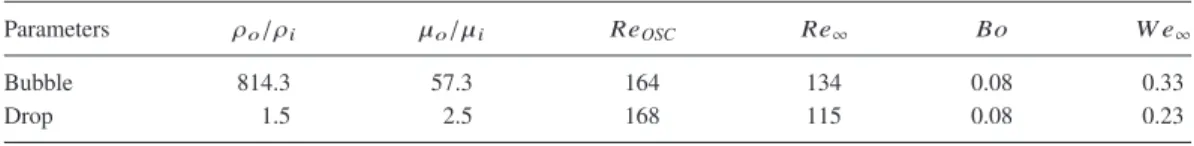
TABLE II. Dimensionless parameters for the two investigated configurations. The terminal velocity used to calculate Re∞ et W e∞is that given by the numerical simulation to ensure that it is not affected by any effect of surface contamination. Parameters ρo/ρi µo/µi ReOSC Re∞ Bo W e∞
Bubble 814.3 57.3 164 134 0.08 0.33 Drop 1.5 2.5 168 115 0.08 0.23
oscillation Reynolds number ReOSC=√ρoσR/µo, based on the characteristic velocity induced by
the oscillationsp σ/(ρoR), and is the reciprocal of the Ohnesorge number. The second is the rising
Reynolds number Re∞= ρoV∞2R/µo based on the terminal velocity V∞. The choice of these two
Reynolds numbers is particularly relevant to assess the role of the rising motion on the oscillations since their ratio compares the characteristic velocities involved in the two kinds of motion. In order to measure the importance of gravity and inertia effects upon the bubble/drop deformation, the Bond number Bo = (ρo−ρi)g (2R)2
σ and the Weber number W e∞= ρoV∞22R
σ are also introduced. The value of
the Bond number is low for both experiments with the bubble and the drop (Bo = 0.08).
Note that in this study, the Reynolds number of oscillation is high enough to consider that shape-oscillations are dominated by inertia, the role of viscous effect being limited to cause a slow damping of the oscillations. Moreover, since ReOSCand Re∞are of the same order of magnitude,
a coupling between the translational and oscillating motions is possible. In addition to the exper-imental Bond number (Bo = 0.08), a case with no gravity (Bo = 0) and a case with augmented gravity (Bo = 0.40) will also be numerically simulated to better analyze this point.
D. Mode extraction
Figs.1(a)and1(b)show several computed shapes of the bubble and of the drop, respectively, superposed on the corresponding image taken in the experiment just before the detachment. The uppermost contour corresponds to the computed terminal shape once the steady motion is reached.
For both the experimental and computational results, the interface contour is extracted and decomposed on the basis of the axisymmetric spherical harmonics, given by the Legendre polyno-mials Plas r(θ, t) = R a0(t) + ∞ X l =2 al(t) Pl(cos θ) , (1)
where r and θ are the spherical coordinates defined in Fig.1(a). The decomposition of the interface is written in the frame of reference in which the amplitude of the first harmonic vanishes, a1=0,
which describes the vertical translation of the inclusion. Note that the normalized amplitude a0of
FIG. 1. (a) Air bubble in water. Experimental picture of the capillary with the bubble just before detachment, superposed with the initial shape for the simulation (yellow) and several other shapes from both the experiment (continuous lines) and the simulation (black symbols) at t = 3Tth
2/2, 4T th 2, 13T th 2/2, and 69T th
2/4 (for terminal shape), T th 2 =2π/ω
th
2 being the theoretical
period of oscillation of mode 2 in the absence of gravity. (b) Heptane drop in water. Experimental picture of the capillary with the drop just before detachment, superposed with the initial shape for the simulation (yellow) and several other shapes from both the experiment (continuous lines) and the simulation (black symbols) at t = 3Tth
2/2, 4T th 2, 13T th 2/2, and 31T th 2/4
TABLE III. Initial non-dimensional amplitudes of the spherical harmonics obtained by fitting the experimental contours by Eq. (1) with l ≤ 12.
al(0) l =0 l =2 l =3 l =4 l =5 l =6 l =7 l =8 l =9 l =10 l =11 l =12
Bubble 0.9904 0.1810 −0.0718 0.0694 −0.0552 0.0458 −0.0451 0.0389 −0.0358 0.0321 −0.0359 0.0263 Drop 0.9912 0.1858 −0.0644 0.0555 −0.0351 0.0273 −0.0232 0.0183 −0.0225 0.0211
harmonic l = 0 is slightly lower than unity since this harmonic ensures volume conservation by compensating for the increase of volume by higher harmonics. In the following, harmonic 0 will be disregarded as its variations are negligible compared to those of the other harmonics.
By decomposing the shape observed in experiments short time before detachment, the initial level-set function for the numerical simulation is obtained. To ensure good accuracy, terms with order up to l = 12 (bubble) and l = 10 (drop) are used. Coefficients describing the initial shape at t = 0 are given in TableIII, and the corresponding shape is also shown in Figs.1(a)and1(b)(lowermost contour). From the time evolution of the amplitude of the different harmonics al(t), we will extract the
frequencies ωl and damping rates βl of the corresponding oscillation modes. These values will be
compared against the values given by the linear theory ωth l and β
th
l , which are computed from the
expressions of Ref.5and given in TableIV.
III. RESULTS FOR THE BUBBLE
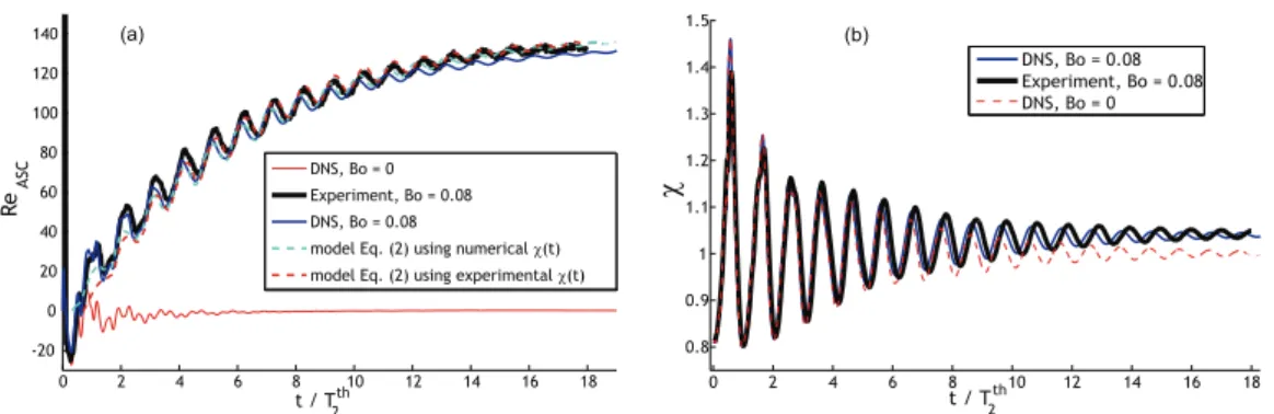
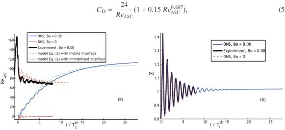
Fig. 2(a) plots time evolution of the Reynolds number ReASC= ρoV (t)2R/µo based on the
instantaneous rise (ascension) velocity V (t) of the center of mass of the bubble, and Fig.2(b)shows the evolution of the aspect ratio χ(t), which is defined as the ratio of horizontal to vertical maximum bubble dimension.
Even though the initial velocity of the bubble is different in the experiment and simulation (the initial velocity in the experiment is about 5% of the terminal velocity because of the impetus received by the bubble from the moving capillary), its evolution is comparable from the beginning of the first oscillation period until reaching the same terminal velocity. Since the simulation assumes a clean interface boundary condition, this demonstrates that the experimental device is clean enough for the drag force to match the case of a non-contaminated bubble. To reinforce this conclusion, let us consider a balance of forces to reconstruct the evolution of the rising velocity. The balance between the added-mass, drag, and buoyancy forces acting on the bubble reads
4 3πR 3 d dt[( ρi+ ρoCM(t)) V (t)] = −ρoCD(t) πR2 2 V (t) 2 + ( ρo− ρi)g 4 3πR 3. (2) At each instant, the added-mass coefficient CMis taken as that of the ellipsoid with the same aspect
ratio χ, given by CM= β0/(2 − β0), with β0=(ζ2+1)ζ cot−1ζ − ζ2and ζ = ( χ2− 1)−1/2. For the
drag coefficient CD, we use the following:
• for ReASC<50, the expression for a spherical bubble given by Mei et al.21is
CbubbleD = 16 ReASC 1 + * , 8 ReASC +1 2 * ,1 + 3.315 Re1/2ASC + -+ -−1 (3)
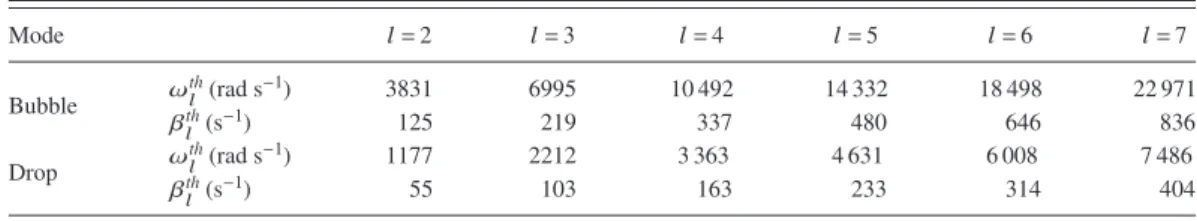
TABLE IV. Theoretical frequencies ωlthand damping rates β th
l for modes l = 2–7, computed from expressions of Ref.5.
Mode l =2 l =3 l =4 l =5 l =6 l =7 Bubble ω th l (rad s−1) 3831 6995 10 492 14 332 18 498 22 971 βth l (s−1) 125 219 337 480 646 836 Drop ω th l (rad s−1) 1177 2212 3 363 4 631 6 008 7 486 βth l (s−1) 55 103 163 233 314 404
FIG. 2. Bubble case. (a) Instantaneous Reynolds number of rising ReASC. (b) Time evolution of the bubble aspect ratio χ.
• for ReASC≥ 50, the expression for a spheroidal bubble given by Moore22is
CD= 48 ReASC G( χ) 1 + H( χ) Re1/2ASC , (4)
where G( χ) and H( χ) are two functions of the aspect ratio given in Moore’s paper.
Using the known evolution of the aspect ratio, either from the experiment or from the numerical simulation, the velocity evolution is obtained by the integration of Eq. (2) and the results are also shown in Fig.2(a). We observe that this model matches well both experimental and numerical re-sults. The possible influence of surface-active contaminants on the bubble motion is thus excluded.
Note that the shape oscillations affect periodically the rising velocity of the bubble due to periodic evolution of its added-mass: velocity oscillates at mode 2 frequency as previously demon-strated in Refs.23 and12. In Fig.2, we also observe that the bubble velocity in the simulation without gravity is not exactly zero. This is due to the presence of odd modes in the deformation that breaks the symmetry between the lower and the upper parts of the bubble and consequently generate small displacements of its center. Nevertheless, this motion is negligible compared to the velocity variations observed in the case with gravity.
Concerning the shape, Fig.2(b)shows that the oscillations cause significant variations of the aspect ratio of the bubble, ranging between 0.8 and 1.5. The bubble oscillates around a mean shape, which remains nearly spherical and flattens only slightly, reaching a final aspect ratio of χ∞=1.04 once the terminal velocity is attained and oscillations decay. Hydrodynamic stresses resulting from the rising motion, which deform the bubble, are of low magnitude (W e∞=0.3); consequently, we observe comparable fluctuation amplitudes of χ in the simulations at Bo = 0.08 and at Bo = 0.
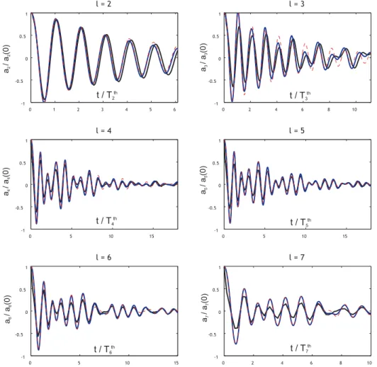
The shape oscillations are studied in detail by decomposing the interface in the basis of the spherical harmonics (Eq. (1)). The evolution of amplitudes for orders l = 2–7 is shown in Fig.3. Amplitudes are normalized by their initial value and time by the theoretical period of oscillation of each mode, Tth
l =2π/ω
th
l. Note that ω th
l increases with the order of the mode: for instance,
ωth 7 ≈ 6 ω
th
2. In Fig. 3, the physical time corresponding to the same dimensionless time is hence
decreasing with the mode order.
The agreement between the experimental and numerical results on the evolution of various harmonics is excellent for lower harmonics. Discrepancies appear for harmonics of higher order (l = 7 or superior), highlighting the limitations of the two approaches used here. In the experi-ments, the main limitation is the temporal resolution. By contrast, in the numerical calculation, this issue can be solved by reducing the time step as necessary. The numerical tool is rather limited by its spatial resolution, which becomes problematic when the oscillation amplitude is low. We have estimated12 that the resolution is sufficient if the oscillation amplitude exceeds 15% of the grid spacing, that is, 0.5% of the undisturbed radius of the particle. We observe in Fig.3that the oscillations are well reproduced whatever the tool is considered and a disagreement appears only at mode 7. Comparisons of Fig.3 suggest that both measured and calculated modes are reliable, including low-amplitude oscillations of harmonics 3-6, which clearly show complex modulations.
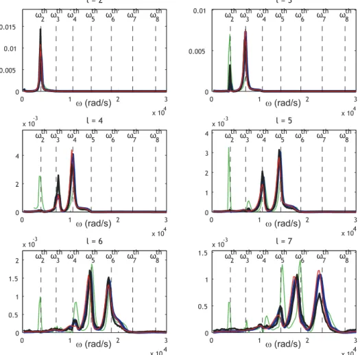
FIG. 3. Bubble case. Time evolution of spherical harmonic amplitudes alfor l = 2–7. Black: Experiments at Bo = 0.08.
Blue: DNS at Bo = 0.08. Dashed red: DNS at Bo = 0.
Note that such results would be questionable if obtained with only one of the approaches. The good agreement of both instantaneous shape and velocity between the experiment and the simulation justifies a deeper investigation of oscillating modes and non-linear effects.
Two other representations are used to characterize the oscillations. Fig.4shows power spectra of the al signals for spherical harmonics l = 2–7, normalized by their variances. The theoretical
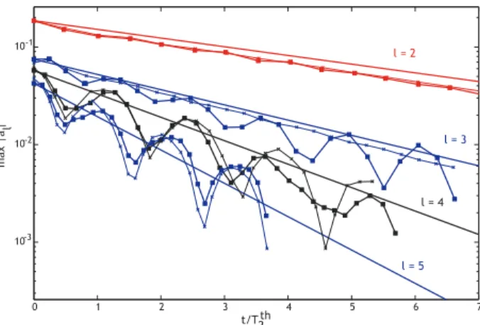
natural frequencies ωthl of modes l = 2–7 are highlighted. Fig.5plots the time evolution of the local
maxima of |al(t)| for l = 2–5 in the both cases without and with gravity (Bo = 0 and Bo = 0.08,
respectively). For clarity purposes, only numerical data are displayed in this figure but experi-mental signals exhibit similar evolutions of local maxima. On this graph, straight lines represent the theoretical damping rates βth
l in the case without gravity.
In Fig.4, the spectrum of each spherical harmonic l exhibits a dominant frequency very close to the theoretical eigenfrequency ωth
l, for harmonics 2–5. For each of these harmonics, secondary
peaks of smaller amplitude occur at lower-order harmonic frequencies. (For harmonic 6 and 7, dominant frequency is no longer the corresponding theoretical frequency but that of the harmonic of adjacent lower order). Figure 5 shows that even though the local extrema of the oscillation amplitudes of each harmonics are not distributed along a straight line, they oscillate around a line corresponding to a constant damping rate βl, which is only about 10% higher than βthl for harmonics
l =2–4. Thus, the linear theory, which (i) does not consider the effect of the rising motion and (ii) assumes oscillations of low amplitudes, still correctly predicts the main trends of the bubble oscillations at moderate amplitudes a2(0) ≈ 0.2 in terms of both dominant frequency and damping
FIG. 4. Bubble case. Power spectra of amplitudes al of spherical harmonics for l = 2–7, normalized by the variance of
the signal. Black: Experiments at Bo = 0.08; blue (thick): simulations at Bo = 0.08; red (thin): simulations at Bo = 0; and green (thin): simulations at Bo = 0.40. Note that for case at Bo = 0.40, the bubble oscillates around an oblate spheroid which flattens slowly with time; this low frequency evolution has been filtered from the oscillations at high frequency when calculating the spectra.
We also observe in Fig.5that the decay of oscillations is comparable for the cases at Bo = 0.08 and Bo = 0, except for harmonic 3 which will be discussed later. This proves that the low discrep-ancy between βland βthl mainly comes from the non-linearity of the oscillations and not from the
rising motion. Hence, gravity can be disregarded in this range of parameters, in accordance with the theoretical study of Meiron24and our previous numerical study.12In particular, we can consider that
the bubble shape oscillates around a spherical shape. Eigenvectors of oscillation modes are therefore the spherical harmonics defined by the Pl polynomials and the eigenfrequencies are given by ωthl .
Consequently, the presence of a secondary frequency ωth
n, with n , l in the alsignal is undoubtedly
the signature of non-linear interactions between the modes. The non-linear coupling between the modes is exhibited by the modulation of amplitude of harmonics 3–7 (Figs.3and5). At Bo = 0.08, Fig.5shows that the extrema of amplitudes of harmonics 3–5 oscillate around an average decay close to βth
l at a frequency that is almost the same for all harmonics and close to that of mode 2. This
suggests periodic energy exchanges between the modes. Remarkably, no perturbation is seen on the amplitude of a2.
As apparent from the spectra (Fig.4), a2is the only harmonic that does not contain any other
frequency than its natural one. This is linked to a more general observation that is valid for all modes: only secondary frequencies corresponding to modes of lower orders are present in the signal of a given mode. For example, signal of harmonic 5 is dominated by ω5but it also contains three
FIG. 5. Bubble case. Symbols: Time evolution of extrema of |al| for l = 2–5, extracted from the numerical signals of the
simulation without gravity (thin lines with crosses) and with gravity (Bo = 0.08, thick lines with squares). Lines without symbols show theoretical damping βth
l from the linear theory without gravity.
lower frequencies, ω4, ω3, and ω2. In return, it does not contain ω6and ω7(Fig.4). Moreover, most
of the energy is distributed on ω5and ω4, peaks at ω2and ω3being small. Interactions between the
modes of very different orders are weak, probably because the fast damping of a high-order mode does not allow it to disturb a low-order mode.
Let us consider now a peculiar characteristic of mode 3, which is the only one that shows a difference between the cases with and without gravity. At Bo = 0, a3is not affected by the presence
of the other modes: it contains a single peak at its natural frequency (Figs.3and4) and its decay is monotonous (Fig.5). On the contrary, at Bo = 0.08, a3shows significant secondary oscillations
at ω2, which also modulates its decay. The weak effect of gravity is therefore both sufficient and
necessary to generate a notable coupling between modes 2 and 3. A possible interpretation of this phenomenon is that the coupling between the odd and even modes requires that the fore-aft symmetry is broken. Since mode 3 is not affected by odd modes of higher order, the slight average deformation generated by the rising motion at Bo = 0.08 is the only way to allow mode 3 to be affected by mode 2. For mode 5, the presence of mode 3 is sufficient to allow the coupling with mode 4. The same argument holds for odd modes of higher orders.
Except for the coupling between modes 2 and 3, gravity does not affect the oscillations at Bo =0.08. An additional simulation at Bo = 0.40 has been carried out in order to show the effect of a significant gravity. In this case, the larger rising velocity of the bubble (Re∞=358, W e∞=2.4) results in a larger and faster deformation of its shape with a terminal aspect ratio χ∞=1.5. The spectra of the oscillation amplitude are shown in Fig. 4. New secondary peaks are present and, in particular, the frequency of harmonic 2 clearly appears in the oscillations of each spherical harmonic until l = 7. However, this is not the signature of enhanced non-linear couplings. As shown from numerical simulations conducted in the linear regime,12the eigenmodes of oscillations around
a shape that is deformed by the rising motion no longer correspond to the spherical harmonics. The decomposition into spherical harmonics is therefore not able to separate the different eigenmodes. In the present case, at Bo = 0.40, the secondary peaks in al spectra result both from the fact that
spherical harmonics do not describe the eigenmodes of oscillations of an oblate bubble and from non-linear couplings between the modes. During the transient rising stage, while the bubble de-forms due to inertia, the oscillating frequency ω2is found to decrease slightly in time compared to
the value without gravity, reaching 0.9 ωth
2 when the bubble rate of deformation no longer evolves,
i.e., when its rising velocity is close to the terminal velocity. This value is consistent with the theo-retical prediction of Meiron24and the numerical result of Lalanne et al.12for a bubble at χ
∞=1.5.
At this time, the damping rate of amplitude of spherical harmonic 2 is measured to be constant, with a value close to βth
2.
To conclude, for the experimental bubble at Bo = 0.08, the analysis of the rising velocity and shape-oscillations reveals that its interface can be considered as clean in experiments since both
experiments and numerical simulations give the same results and compare well with the model incorporating the drag force that corresponds to the contaminant-free case. Effect of buoyancy on the oscillations is globally negligible (except on the coupling of oscillations of harmonics 3 and 2), because the terminal shape of the bubble is nearly spherical, so that the eigenmodes of oscillation correspond to the spherical harmonics. The dominant frequency of each mode is given by the linear theory without gravity, whereas its global damping rate is only 10% larger than the linear prediction. Non-linear couplings between the different modes of oscillation have been analyzed from the spectra of each spherical harmonic and the temporal decay of its amplitude. Modes of lower frequency influence modes of higher frequency, whereas the reverse is not observed.
IV. RESULTS FOR THE DROP
We consider now the case of the liquid drop. Figs.6(a)and6(b)show the time evolutions of ReASC
and χ in the experiment and in the simulations for Bo = 0.08 and Bo = 0. The origin of time has been defined as the instant of detachment of the drop from the capillary. The experimental evolution of ReASCfor negative times illustrates what happened before the drop release: the capillary moves up
and down and the detachment of the drop takes place during the deceleration stage. Contrary to the previous experiment with the bubble, the initial velocity of the drop at the instant of detachment is large and even exceeds the terminal rising velocity. The initial condition in the simulation (with zero velocity) is hence significantly different from the experimental condition in this case. Nevertheless, different initial conditions for velocity should not cause differences between the results once the ter-minal velocity, which is governed by the equilibrium between buoyancy and drag forces, is attained. Yet, we observe in Fig.6(a)that the experimental terminal rising velocity is only 60% of the terminal velocity in the simulation. This discrepancy suggests that surface-active contaminants are adsorbed at the drop interface and they partially immobilize it by being convected to the rear of the drop; it results in an increase of the drag that becomes comparable to that exerted at the surface of a solid particle exactly like if the interface was fully immobilized.25However, this residual contamination induces a
negligible variation of surface tension between heptane and water, since we find the value for a clean interface. To confirm the presence of surfactant in the experiment, we reconstruct the time evolution of the drop velocity using the force balance between buoyancy, drag, and added-mass forces during the unsteady rising motion of the drop. The force balance is the same as for bubbles, given by Eq. (2). The added-mass cœfficient CMis calculated from the aspect ratio χ(t) in the same way as for the bubble,
and the value of χ(t) is taken either from the experiment or from the Direct Numerical Simulation (DNS) results. The expressions of the drag coefficient CDare chosen as follows:
• for the experimental case, we use the drag coefficient of a solid sphere proposed by Schiller and Naumann,26to assess the assumption of a contaminated interface,
CD=
24 ReASC
(1 + 0.15 Re0.687ASC ), (5)
• for the numerical case, we use the correlation of Rivkind and Ryskin27 valid for a spherical drop with a clean interface,
CD= CDbubble+ µi/µoC solid sphere D 1 + µi/µo , (6) where Cbubble
D is the drag coefficient of a spherical bubble
20(Eq. (4)), and Csolid sphere
D is the drag
coefficient of a solid sphere26(Eq. (5)).
Evolutions of the rising velocity obtained by solving the analytical model of force balance (2) for both experimental and the numerical cases (using their corresponding initial velocity: that measured at the instant of detachment for the experimental case, zero for the numerical case) are plotted in Fig.6(a). It can be shown that this model reproduces well both the experimental results with contaminated-interface assumption (black and dashed red curves) and the numerical results with clean-contaminated-interface assumption (dark and dashed light blue curves); thus, it contains the main physics of the problem. The rising velocity oscillates slightly at frequency ωth
2due to varying added-mass CM, but these oscillations
are of lower amplitude than in the bubble case as a consequence of a higher density ρiof the inner fluid.
The small discrepancy that exists between measured or simulated velocity and that from the model comes from neglecting the effect of drop deformation on the drag coefficient and also from neglecting the history force in the force balance (which is more important than in the case of bubbles). However, the agreement of the model with our results allows us to conclude that the presence of surfactants explains the slower rising velocity in the experiments by immobilizing the interface, leading to a drag force similar to that of a solid sphere.
Fig.6(b)shows that the oscillations cause large variations of χ, ranging between 0.8 and 1.4. Surprisingly, in spite of interface contamination, the evolution of χ is the same in the experiment and in the simulation, indicating that the contaminants do not affect significantly the drop-shape dynamics in the experiment. It also confirms that they are present in residual concentration only, which is consistent with the fact that the measured interfacial tension is close to that of a clean interface. The drop shape has an aspect ratio of χ∞=1.02 after reaching its steady rise, consistent with the low values of Bond and
Weber numbers, Bo = 0.08 and W e∞=0.23. The buoyancy forces are hence not sufficiently intense
compared to the surface tension forces to deform significantly the drop and consequently, the time evolution of χ in the simulation without gravity is the same as in the case at Bo = 0.08.
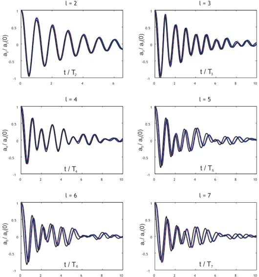
To analyse more precisely the shape oscillations of the drop, let us consider in Fig. 7 the decomposition of its shape into spherical harmonics (Eq. (1)), at each instant of measurement or calculation done at Bo = 0.08. Results of the simulation without gravity are also included in the figure and time has been normalized by the measured frequency of the different harmonics (which is, and discussed later). Graphs of Fig.7show an excellent agreement between the exper-imental and numerical results, including the high order spherical harmonics with low amplitudes (cf. Table III). This confirms the ability of both experimental and numerical tools to handle the non-linear oscillations of the drop. A strong conclusion can be drawn: the contamination by resid-ual surfactants, responsible of the low value of the experimental drop terminal velocity, does not affect the shape-oscillations dynamics in present experiments, for none of the studied spherical har-monics. As it has been previously demonstrated by Abi Chebel et al.,13non-ultrapure experimental
conditions affect the shape-oscillation dynamics through an increase of the damping rate of oscilla-tions, whereas in cleaner conditions (like those in present experiments), shape oscillation dynamics recover those predicted by theories for contaminant-free interface, even though the terminal rising velocity is affected by residual contamination. The fact that (i) we observe an increase of the dissi-pation of the energy associated to the rising motion due to surface contamination and (ii) we do not observe an increase of the dissipation of the energy associated to the oscillating motion is probably related to the location where dissipation of energy takes places. For rising drops, energy of the translating motion is mainly dissipated in a boundary layer that develops along the interface and in the drop wake. For oscillating drops, the linear theory of oscillation (Ref.5) shows that dissipation is mainly due to the existence of an oscillating boundary layer close to the interface (see Fig. 8(a) of Ref.12for an illustration). Our observations lead us to think that the boundary layer associated with rising motion and that associated with interface oscillations have a distinct dynamics since they are
FIG. 7. Drop case. Time evolution of spherical harmonic amplitudes alfor l = 2–7. Black: Experiments at Bo = 0.08. Blue:
DNS at Bo = 0.08. Dashed red: DNS at Bo = 0.
differently affected by contaminants. Further investigations of these boundary layers are required to validate this interpretation.
In accordance with the observed evolution of the aspect ratio, simulations at Bo = 0.08 and Bo =0 provide a very similar behavior for all alsignals, confirming that the effect of gravity and
of rising motion on shape-oscillations are negligible at Bo = 0.08. This is consistent with the fact that comparable oscillations at Bo = 0.08 are obtained in the experiment and in the simulation, even though the rising velocity is very different in the two cases. Indeed, the Weber number is too low to induce an effect of the rising motion on the oscillation dynamics (as already shown in Ref.12in the case of linear oscillations). Therefore, the mean shape around which the drop oscillates is almost a sphere with a negligible deformation at steady state (a2= −0.012). Consequently, the eigenmodes
of oscillation still coincide with the spherical harmonic basis, as it is the case at Bo = 0, and the oscillation dynamics is not influenced by gravity.
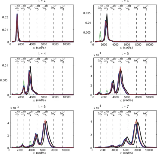
The same representations as for the bubble case are used to characterize the oscillations of the different harmonics. Frequencies are analyzed from the power spectra of the alsignals for l = 2–7
(Fig.8), and the time evolutions of the local extrema of |al(t)| (Fig.9) allow us to characterize the
damping rates of the oscillation amplitudes for harmonics l = 2–5. We compare again measured ωl and βl with the linear theory of oscillation and we investigate the non-linear effects and the
FIG. 8. Drop case. Power spectra of amplitudes alof spherical harmonics for l = 2–7, normalized by the variance of the
signal. Black: Experiments at Bo = 0.08; blue (thick): simulations at Bo = 0.08; red (thin): simulations at Bo = 0; and green (thin): simulations at Bo = 0.40. Note that for case at Bo = 0.40, the drop oscillates around an oblate spheroid which flattens slowly with time; this low frequency evolution has been filtered from the oscillations at high frequency when calculating the spectra.
Concerning the dominant frequency in each power spectrum, both the numerical simulation (at Bo = 0.08 and Bo = 0) and the experiment are in agreement with ωth
l for all harmonics within
the expected accuracy, ranging between 0.5% and 5% depending on the value of l.
Concerning the global damping rates, experiment and simulation are again in good agreement with a discrepancy of 3% for harmonics l = 2–4 and show that a2 and a3 decay at a rate higher
by 8% than βthl. Since the same value of β2is found in the simulations at Bo = 0.08, at Bo = 0,
and in the experiment, we can attribute this slight increase of the damping rate of mode 2 to non-linear effects that are not considered in the theory. Nevertheless, an increase of 8% is moderate compared to the influence of gravity or surfactants which have been shown to increase the damp-ing rate β more radically (by a factor of two or three) at larger Bond numbers12 or in less clean
conditions.13
The linear theory hence provides correctly the main trends of frequency and global damping rates of the oscillations, which remain close to ωth
l and β th
l . Non-linear effects in the oscillations are
however noticeable. In Fig.8, the presence of several frequencies is visible in harmonics 4–7. This reveals the couplings between the modes, which is identical in the experiment and in the simulation at Bo = 0.08. As in the case of the bubble, only secondary frequencies of modes of lower orders are visible in the spectrum of a given mode. In particular, non-linear interactions are not detected in the dynamics of mode 2.
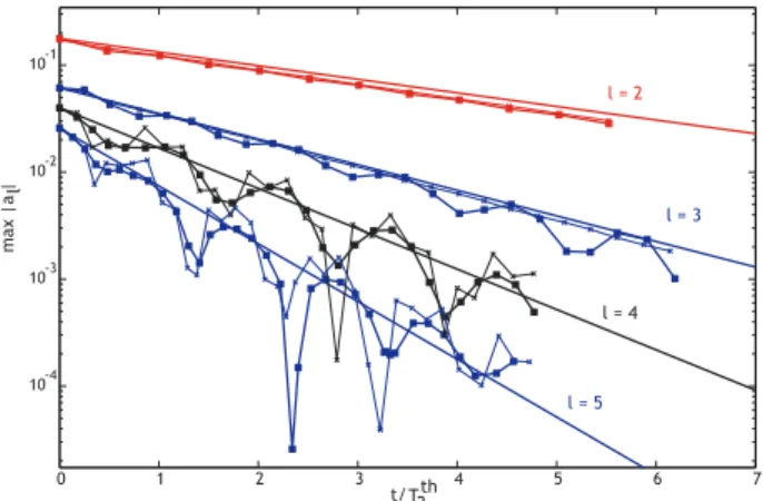
FIG. 9. Drop case. Symbols: Time evolution of the absolute values of the extrema of |al| for l = 2–5, extracted from the
numerical signals of the simulation without gravity (fine lines with crosses) at Bo = 0 and with gravity (thick lines with squares) at Bo = 0.08. Lines: Theoretical damping βth
l from the linear theory.
In Fig.9, we observe that non-linear mode coupling results in modulations of the decay rate of a given mode. These modulations have the same dominant frequency for l = 3 and l = 4 and this frequency is close to ωth2, as in the bubble case. Amplitude variations at Bo = 0.08 and Bo = 0 are similar, except for mode 3. This suggests again that the coupling between the odd and even modes requires the breaking of the fore-aft symmetry.
An additional simulation has been carried out for augmented-gravity condition (Bo = 0.40). This simulation has been stopped before the drop has reached its terminal velocity, at time t∗=8Tth
2 ,
when the rising Reynolds number of the drop is ReASC(t∗) = 278 and its mean aspect ratio is
χ(t∗) = 1.15. The global damping of the oscillations β2is observed to increase as the drop
accel-erates, reaching a value of 1.3 βth
2 at t∗when the instantaneous Weber number is W e(t∗) = 1.4, in
agreement with Fig. 7(b) of Ref.12. Even if the deformation of the mean shape remains moderate, it is sufficient to change the eigenmodes of oscillations that no longer correspond to the spherical harmonics. Consequently, the spectra of alsignals (especially those for l = 3–5) exhibit several low
frequencies that are not present at Bo = 0.08: the peak at ωth
2 in the signal of harmonic 3 becomes
significant and ωth 2 and ω
th
3 appear in harmonics 4 and 5.
To summarize, in the case of the drop at Bo = 0.08, the comparison between the simulation and experiment proves that, despite all the precautions taken to clean the experimental device, the inter-face is contaminated. This strongly affects the rising motion but does not have any significant effect on the shape-oscillation dynamics of the drop. The analysis of these shape-oscillations through a modal decomposition shows the existence of interactions between the modes due to their initial amplitudes reaching 0.2R. Nevertheless, the dominant frequency and the global damping rate of each mode of oscillation are still accurately predicted by the linear theory of oscillation. The gravity effects can be disregarded for the shape-oscillations of that drop (except for a non-linear effect of second order visible on the oscillation amplitude of mode 3).
V. CONCLUSION
This study has compared experimental observations and numerical simulations of a rising bubble or a drop, the shape of which oscillates. Despite some differences in the initial conditions between the simulation and the experiment (non-initialized-fluid velocities and truncated series describing the initial shape), a good agreement between the results validates both approaches. An interest in performing such a comparison is to separate the influence of various factors, which are all involved in the experiment, but are easily discriminated only in a simulation. This methodology has been applied here to interpret the experimental results (i) to conclude on the degree of contami-nation of the fluids in the experimental device and on the effect of this contamicontami-nation on oscillation
dynamics, and (ii) to assess the influence of gravity, in order (iii) to finally analyze the existence of non-linear couplings in the shape oscillations of a bubble and a drop.
Concerning contamination, the comparison has shown that the shape oscillations observed in experiments do not differ from pure conditions for both the bubble and the drop, though the drop rising velocity corresponds to the case of a drop with immobilized interface suggesting a residual contamination. To our knowledge, experiments in which the rising velocity of a drop corresponds to that of a drop with clean interface have not been reported. However, the present results indicate that it is easier to obtain experimentally a drop that oscillates as a clean drop, rather than a drop that reaches the rise velocity of an uncontaminated drop.
Concerning effects of gravity on millimeter-sized bubbles and drops, the simulations allow us to conclude that buoyancy does not affect significantly the interface dynamics provided the mean oscillating shape remains close to a sphere (as it is the case here), even though the rising and oscillating velocities are of the same order. Thus, it is still relevant to decompose the interface shape in spherical harmonics, which correspond to the eigenmodes of the oscillations.
Concerning the oscillation nonlinearities, couplings between the modes are easily observable from the temporal evolution and the spectrum of amplitudes of the different spherical harmonics. Exchanges of energy induce modulations at mode 2 frequency in the temporal decay of the oscilla-tion amplitude associated with each mode. Nevertheless, for initial amplitudes of magnitude of 0.2R like those of our experiments, the dominant frequency and the global decay rate associated with each mode of oscillation are still accurately given by the linear theory, with a maximum discrepancy of 10% for the damping rate.
Thus, using such a complementarity between the experimental and numerical results in this paper, it has been demonstrated that it is easy to produce shape oscillations for rising drops or bubbles that are not influenced by buoyancy. This result might avoid the need for costly experiments in micro-gravity conditions, for example. Bubble or drop oscillations might also be considered for an investigation of the interface dynamics in more complex situations, e.g., in the presence of surfactants at non-negligible concentrations.
ACKNOWLEDGMENTS
The experiments have been carried out with support of Ministry of Education, Youth and Sports of the Czech Republic (Project No. LD 13018).
1I. S. Kang and L. G. Leal, “Bubble dynamics in time-periodic straining flows,”J. Fluid Mech.218, 533–542 (1990). 2F. Risso and J. Fabre, “Oscillations and breakup of a bubble immersed in a turbulent field,”J. Fluid Mech.372, 323–355
(1998).
3S. Galinat, F. Risso, O. Masbernat, and P. Guiraud, “Dynamics of drop breakup in inhomogeneous turbulence at various
volume fractions,”J. Fluid Mech.578, 85–94 (2007).
4C. A. Miller and L. E. Scriven, “The oscillations of a fluid droplet immersed in another fluid,”J. Fluid Mech.32, 417–435
(1968).
5A. Prosperetti, “Normal mode analysis for the oscillations of a viscous liquid drop in an immiscible liquid,” Journal de
Mécanique 19, 149–182 (1980).
6A. Prosperetti, “Free oscillations of drops and bubbles: The initial-value problem,”J. Fluid Mech.100, 333–347 (1980). 7M. Strani and F. Sabetta, “Free vibrations of a drop in partial contact with a solid support,”J. Fluid Mech.141, 233–247
(1984).
8M. Strani and F. Sabetta, “Viscous oscillations of a supported drop in an immiscible fluid,”J. Fluid Mech.189, 397–421
(1988).
9J. Bostwick and P. H. Steen, “Capillary oscillations of a constrained liquid drop,”Phys. Fluids21, 032108 (2009). 10A. Prosperetti, “Linear oscillations of constrained drops, bubbles, and plane liquid surfaces,”Phys. Fluids24, 032109 (2012). 11H. L. Lu and R. E. Apfel, “Shape oscillations of drops in the presence of surfactants,”J. Fluid Mech.222, 351–368 (1991). 12B. Lalanne, S. Tanguy, and F. Risso, “Effect of rising motion on the damped shape oscillations of drops and bubbles,”Phys.
Fluids25, 112107 (2013).
13N. Abi Chebel, J. Vejražka, O. Masbernat, and F. Risso, “Shape oscillations of an oil drop rising in water: Effect of surface
contamination,”J. Fluid Mech.702, 533–542 (2012).
14N. Otsu, “Threshold selection method from gray-level histograms,”IEEE Trans. Syst. Man Cybern.9(1), 62–66 (1979). 15M. Sussman, M. Smereka, and S. Osher, “A level-set approach for computing solutions to incompressible two-phase flows,”
J. Comput. Phys.114, 146–159 (1994).
16M. Sussman, K. M. Smith, M. Y. Hussaini, M. Ohta, and R. Zhi-Wei, “A sharp interface method for incompressible two-phase
17X.-D. Liu, R. P. Fedkiw, and M. Kang, “A boundary condition capturing method for Poisson’s equation on irregular domains,” J. Comput. Phys.160, 151–178 (2000).
18S. Tanguy and A. Berlemont, “Application of a level-set method for simulation of droplet collisions,”Int. J. Multiphase Flow31, 1015–1035 (2005).
19B. Lalanne, L. Rueda Villegas, S. Tanguy, and F. Risso, “On the computation of viscous terms for incompressible two-phase
flows with level set/ghost fluid method,”J. Comput. Phys.301, 289–307 (2015).
20D. W. Moore, “The boundary layer on a spherical gas bubble,”J. Fluid Mech.16, 161 (1963).
21R. Mei, J. F. Klausner, and C. J. Lawrence, “A note on the history force on a spherical bubble at finite Reynolds number,” Phys. Fluids6, 418–420 (1994).
22D. W. Moore, “The velocity of rise of distorted gas bubbles in a liquid of small viscosity,”J. Fluid Mech.23, 749 (1965). 23J. de Vries, S. Luther, and D. Lohse, “Induced bubble shape oscillations and their impact on the rise velocity,”Eur. Phys. J.
B29, 503–509 (2002).
24D. I. Meiron, “On the stability of gas bubbles rising in an inviscid fluid,”J. Fluid Mech.198, 101–114 (1989).
25B. Cuenot, J. Magnaudet, and B. Spennato, “The effect of sligthly soluble surfactants on the flow around a spherical bubble,” J. Fluid Mech.339, 25–53 (1997).
26L. Schiller and A. Naumann, “A drag coefficient correlation,” Z Vereines Deutscher Ingenieure 77, 318–320 (1935). 27V. Y. Rivkind and G. Ryskin, “Flow structure in motion of a spherical drop in a fluid medium at intermediate Reynolds