Evaluation of lichen species resistance to atmospheric metal pollution by coupling diversity and bioaccumulation approaches: A new bioindication scale for French forested areas

O

pen

A

rchive

T

OULOUSE

A

rchive

O

uverte (

OATAO

)

OATAO is an open access repository that collects the work of Toulouse researchers and

makes it freely available over the web where possible.

This is an author-deposited version published in :

http://oatao.univ-toulouse.fr/

Eprints ID : 17390

To link to this article : DOI:

10.1016/j.ecolind.2016.08.006

URL :

http://dx.doi.org/10.1016/j.ecolind.2016.08.006

To cite this version :

Agnan, Yannick and Probst, Anne and

Séjalon-Delmas, Nathalie Evaluation of lichen species resistance to

atmospheric metal pollution by coupling diversity and

bioaccumulation approaches: A new bioindication scale for French

forested areas. (2017) Ecological Indicators, vol. 72. pp. 99-110.

ISSN 1470-160X

Any correspondence concerning this service should be sent to the repository

administrator:

staff-oatao@listes-diff.inp-toulouse.fr

Evaluation of lichen species resistance to atmospheric metal pollution

by coupling diversity and bioaccumulation approaches: A new

bioindication scale for French forested areas

Y. Agnan

, A. Probst

, N. Séjalon-Delmas

a_{ECOLAB, Université de Toulouse, CNRS, INPT, UPS, France}

b_{Milieux Environnementaux, Transferts et Interactions dans les hydrosystèmes et les Sols (METIS), UMR 7619, Sorbonne Universités UPMC-CNRS-EPHE, 4} place Jussieu, F-75252 Paris, France

c_{Laboratoire de Recherche en Sciences Végétales (LRSV), Université de Toulouse, UPS, CNRS, 31326 Castanet-Tolosan, France}

Keywords: Diversity Resistance scale Sensitivity Metal Forest Atmospheric purity

a b s t r a c t

In order to evaluate the metal resistance or sensitivity of lichen species and improve the bioindication scales, we studied lichens collected in eight plottings in French and Swiss remote forest areas. A total of 92 corticolous species was sampled, grouped in 54 lichen genera and an alga. Various ecological variables were calculated to characterize the environmental quality – including lichen diversity, lichen abundance, and Shannon index –, as well as lichen communities. Average ecological features were estimated for each study site and each of the following variables – light, temperature, continentality, humidity, substrate pH, and eutrophication – and they corresponded to lichen communities. Based on lichen frequencies, we calculated the index of atmospheric purity (IAP) and lichen diversity value (LDV). These two bioindication indices were closely related to lichen diversity and lichen abundance, respectively, due to their calcula-tion formula. It appeared that LDV, which measures lichen abundance, was a better indicator of metal pollution than IAP. Coupling lichen diversity and metal bioaccumulation in a canonical correspondence analysis, we evaluated the resistance/sensitivity to atmospheric metal pollution for the 43 most frequent lichen species. After validation by eliminating possible influences of acid and nitrogen pollutions, we proposed a new scale to distinguish sensitive species (such as Physconia distorta, Pertusaria coccodes, and Ramalina farinacea) from resistant species (such as Lecanactis subabietina, Pertusaria leioplaca, and Pertusaria albescens) to metal pollution, adapted to such forested environment.

1. Introduction

Atmospheric deposition of chemicals impacts natural ecosys-tems over a long-term, and biological species are more or less

susceptible to these pollutants (Schulze et al., 1989; Tyler, 1989).

Lichens are considered sensitive organisms because of their biolog-ical features. The absence of protective cuticle or root system results in a high sensitivity to anthropogenic disturbances, such as

atmo-spheric pollutants (Bajpai et al., 2010; Conti and Cecchetti, 2001;

Shukla et al., 2014; Szczepaniak and Biziuk, 2003). The loss of lichen diversity constitutes one of the main markers of atmospheric pol-lution on the biosphere, as revealed since the first observations in

∗ _{Corresponding authors at: ECOLAB, Université de Toulouse, CNRS, INPT, UPS,} France.

E-mail addresses:yannick.agnan@biogeochimie.fr(Y. Agnan), nathalie.delmas@lrsv.ups-tlse.fr(N. Séjalon-Delmas).

the late 19th century in Paris (Nylander, 1866). Because assessment

of atmospheric pollution is complex and expensive, biomonitoring is a helpful support technique. Several biomonitoring approaches are used to evaluate the level of atmospheric pollution, in relation

to lichen diversity (i.e., bioindication;Geiser and Neitlich, 2007;

Pinho et al., 2004) or accumulation of pollutants (i.e.,

bioaccumu-lation;Conti et al., 2011; Hissler et al., 2008). Lichens are relatively

good candidates frequently used to monitor atmospheric

depo-sition in various environmental contexts: e.g., forested (Gauslaa,

1995; Giordani et al., 2012), rural (Bosch-Roig et al., 2013; Vonarb et al., 1990), and urban (Gombert et al., 2004; Loppi et al., 2004) areas.

Atmospheric acid deposition in Europe several decades ago,

linked to man-made SO₂ and NOx emissions, was responsible

for several disturbances on forest diversity (Schulze et al., 1989).

More specifically, many authors reported that some lichen species have disappeared because of their susceptibility to acid

pollu-tants (Piervittori et al., 1997; Sigal and Johnston, 1986). In this

context, a first biomonitoring scale was developed in England

and Wales byHawksworth and Rose (1970), associating common

lichen species for different atmospheric SO2concentrations. More

recently, in Germany,Wirth (1991)developed a toxitolerance index

for more than 750 lichen species also based on the acid

pollu-tion criteria. With the generalized decrease of SO2concentration

in the atmosphere since the 1980′_{s (Berge et al., 1999), a change}

in biomonitoring scale was needed. Several scales were devel-oped following the relative importance of nitrogen compounds in

the atmosphere (i.e., NOx and NH₄; Lallemant et al., 1996; van

Haluwyn and Lerond, 1993). Nevertheless, these various scales do not take into account other pollutants such as metals (e.g., lead, zinc, cadmium) or organic pollutants (e.g., polycyclic aromatic hydrocarbons [PAH] and polychlorinated biphenyl [PCB]), and lit-tle is known about the sensitivity or resistance to such pollutants for lichen species commonly found in northern countries. Conse-quently, the development of new scales integrating these changes in sulfur and nitrogen compounds as background levels and the occurrence of emerging pollutants is therefore required.

In the meantime, several indices of atmospheric air quality were established based on lichen richness and abundance, such as the

lichen diversity value (LDV;Asta et al., 2002) and the index of

atmospheric purity (IAP;LeBlanc and Sloover, 1970). These indices

attempt to evaluate a general degree of atmospheric pollution. The limit of such indices, however, is that they do not point to the exact pollutants caused by disturbance. A qualitative ecological char-acterization of lichen occurrence should also be employed as an additional tool to complete the quantitative evaluation, as being more frequently done.

In this study, we sampled lichen species in open forest sites from various remote regions of France and neighboring country to characterize the current degree of recent atmospheric pollution based on several approaches of lichen biomonitoring. Assuming a response to a gradient of metal bioaccumulation on lichen richness and abundance, our main objective was to evaluate the resis-tance/sensitivity of lichen species to atmospheric metal pollution by coupling both lichen diversity and bioaccumulation of metals in a multivariate analysis, and to propose a new resistance/sensitivity scale adapted to present-day environmental conditions to further assess the critical loads using lichens.

2. Materials and methods 2.1. Study area

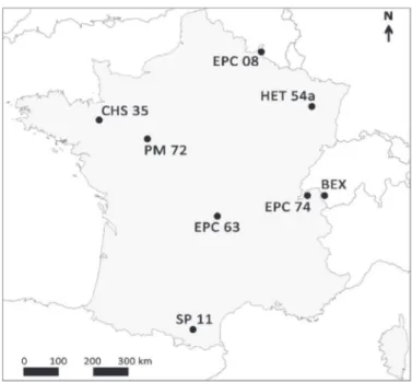
Eight unmanaged open-forested sites were monitored, of which seven sites from various regions of France, and one site located

in Switzerland (Fig. 1). The French sites (SP 11, EPC 63, EPC 74,

HET 54a, EPC 08, PM 72, and CHS 35) belong to the French moni-toring network of forest ecosystems RENECOFOR (Réseau National de suivi des Écosystèmes Forestiers), which is part of the Inter-national Cooperative Programme Forest network (ICP-Forest). The sites included both coniferous forests (Abies alba Mill. in SP 11, Picea abies (L.) H. Karst in EPC 63, EPC 74, and EPC 08, and Pinus pinaster Aiton in PM 72) and hardwood forests (Quercus petraea (Matt.) Liebl. in CHS 35 and Fagus sylvatica L. in BEX and HET 54a). Despite the dominant trees, a mixed of species were found with generally both coniferous and hardwood trees in each study site.

The sites considered various environmental conditions (Table 1).

The elevation was from 80 m a.s.l for CHS 35–1210 m a.s.l for EPC 74. The Northwestern sites (PM 72 and CHS 35) were influenced by an oceanic climate with low annual precipitation (<840 mm), while the Northeastern (HET 54a and EPC 08) and central (EPC 63) ones were under semi-continental climate. The climate was more of mixed influences for the mountainous sites (SP 11, EPC 74, and

Fig. 1. Location of the study sites sampled for lichen diversity: seven sites are located in various regions of France and one in nearby Switzerland.

BEX). Several types of bedrock were concerned, from sedimentary (limestone or sandstone) to magmatic (basalt) substratum.

Metal atmospheric pollution has already been studied for these

sites through surface horizons of soils (Gandois et al., 2010a;

Hernandez et al., 2003), bulk atmospheric deposition (Gandois et al., 2010b), and lichen bioaccumulation (Agnan et al., 2015). The metal concentrations registered in lichens collected on the

trees considered for bioindication are given inTable 2. Differences

between sites were observed with a higher anthropogenic influ-ence in the North-Eastern part of the country, particularly for Pb and Cd in EPC 08, while a greater dust deposition was observed in the Southern regions (e.g., in SP 11). The availability of lichen bioaccumulation data (i.e., metal concentrations in lichens though accumulation from the environment) was a central part of this study to determine both lichen resistance and lichen sensitivity in coupling lichen diversity to the degree of metal concentrations. 2.2. Sampling procedure

Because microclimate and bark properties are known to

influ-ence lichen diversity (Ellis, 2012; Giordani, 2006), each study

site encompassed a representative area of about 250000 m2 _in

open field at the edge of a forest to both maximize the number

of sampling species and preserve the forest influence (Poliˇcnik

et al., 2008). Twelve trees avoiding young and disturbed specimens

for lichen sampling (i.e., circumference > 40 cm, inclination < 10◦_,

trunk without mosses and damages) of various species were

sam-pled (Bargagli and Nimis, 2002; Giordani et al., 2011), including

both deciduous and coniferous trees (Table 1) to improve the

repre-sentativeness of local lichen diversity (Daillant et al., 2007; Deruelle

and Garcia Schaeffer, 1983). We followed the standardized

Euro-pean protocol (EN 16413, 2014), leaving the random sampling to

maximize the number of lichen species by increasing the tree

diver-sity (Moreau et al., 2002). Since we aimed to evaluate the metal

resistance and sensitivity of lichens by combining bioaccumulation and diversity approaches, we thus followed the same procedure

as for bioaccumulation study (Agnan et al., 2015). The four

cardi-nal points of the tree trunks were sampled using a ladder grid of

five vertical squares of 10 cm × 10 cm to cover an area of 500 cm2

Table 1

Summary of geographical and environmental characteristics for each study sites. site coordinates elevation (m) annual

precipitation (mm)

lithology tree species sampled

SP 11 2◦₀₅′₄₀′_{’E/ 42}◦₅₂′₁₅′_{’N 990 1200 limestome/marble Abies alba Mill., Corylus avellana L.,} Fagus sylvatica L., Fraxinus excelsior L., Malus pumila Mill.

EPC 63 2◦₅₈′₀₅′_{’E/ 45}◦₄₅′₀₀′_{’N 950 1100 basalt Crataegus monogyna Jacq., Fraxinus excelsior L.,} Picea abies (L.) Karst., Pinus sp.

EPC 74 6◦₂₁′₀₀′_{’E/ 46}◦₁₃′₃₀′_{’N 1210 1300 sandstone/schist Abies alba Mill., Acer sp., Fagus sylvatica L.,} Picea abies (L.) Karst.,

Prunus avium L., Salix sp., Sorbus aucuparia L. BEX 6◦₅₈′₃₀′_{’E/ 46}◦₁₃′₀₀′_{’N 945 1000 limestone/schist Acer sp., Betula pendula Roth, Fagus sylvatica L.,}

Fraxinus excelsior L., Salix sp.

HET 54a 6◦₄₃′₁₀′_{’E/ 48}◦₃₀′₅₀′_{’N 320 900 limestone Fagus sylvatica L., Fraxinus excelsior L., Quercus sp.} EPC 08 4◦₄₇′₅₀′_{’E/ 49}◦₅₇′₀₀′_{’N 475 1300 clay loam Betula pendula Roth, Corylus avellana L.,}

Fagus sylvatica L., Picea abies (L.) Karst., Prunus avium L., Quercus sp., Rhus hirta (L.) Sudw., Salix caprea L., Syringa vulgaris L.

PM 72 0◦₂₀′₀₀′_{’E/ 47}◦₄₄′₂₅′_{’N 155 800 schist Castanea sativa Mill., Pinus pinaster Ait.,} Quercus petraea (Mattus.) Liebl., Quercus rubra L. CHS 35 1◦₃₂′₅₀′_’W/48◦₁₀′₁₀′_{’N 80 840 clay Fagus sylvatica L., Pinus pinaster Ait.,}

Quercus petraea (Mattus.) Liebl.

Table 2

Summary of metal bioaccumulation (mean ± standard deviation, in mg g−1_{) in three foliose lichen species (i.e., X. parietina, P. sulcata, and H. physodes) from the investigated} forest areas (fromAgnan et al., 2015).

element SP 11 EPC 63 EPC 74 BEX HET 54a EPC 08 PM 72 CHS 35

Al 2364.1 ±1054.3 988.3 ±299.4 1126.7 ±412.0 1157.9 ±277.8 192.4 ±603.1 1072.7 ±591.1 426.1 ±46.0 397.7 ±62.2 As 0.7 ±0.2 0.7 ±0.4 0.3 ±0.1 0.3 ±0.0 0.3 ±0.1 0.6 ±0.2 0.2 ±0.0 0.2 ±0.0 Cd 0.1 ±0.0 0.1 ±0.0 0.7 ±0.7 0.1 ±0.1 0.2 ±0.2 0.6 ±0.1 0.4 ±0.1 0.1 ±0.1 Co 0.4 ±0.2 0.3 ±0.1 0.4 ±0.1 0.3 ±0.1 0.3 ±0.1 0.4 ±0.1 0.1 ±0.0 0.2 ±0.0 Cr 3.7 ±1.3 2.2 ±1.0 1.8 ±0.6 2.8 ±1.0 1.8 ±0.7 2.5 ±0.9 0.8 ±0.1 0.7 ±0.1 Cs 0.3 ±0.1 0.3 ±0.2 0.2 ±0.1 0.2 ±0.1 0.2 ±0.1 0.2 ±0.1 0.1 ±0.0 0.1 ±0.0 Cu 4.7 ±0.9 6.9 ±2.1 10.4 ±3.2 7.1 ±2.4 7.9 ±3.1 7.3 ±1.0 7.2 ±1.0 5.1 ±1.5 Fe 1347.1 ±595.6 759.1 ±262.2 618.5 ±208.4 687.0 ±158.2 617.6 ±334.8 631.0 ±328.5 278.6 ±35.7 240.9 ±36.4 Mn 29.3 ±14.6 25.1 ±4.0 142.0 ±126.8 102.7 ±74.7 69.5 ±73.2 45.7 ±11.3 45.3 ±4.4 346.8 ±117.7 Ni 1.7 ±0.5 1.3 ±0.5 2.1 ±0.7 2.1 ±0.7 1.7 ±0.6 2.0 ±0.3 0.6 ±0.1 1.4 ±0.3 Pb 2.3 ±1.5 2.5 ±1.1 7.3 ±3.5 5.1 ±2.7 16.1 ±13.4 5.2 ±1.1 1.5 ±0.3 6.2 ±10.4 Sb 0.1 ±0.1 0.1 ±0.0 0.1 ±0.0 0.2 ±0.0 0.2 ±0.1 0.3 ±0.1 0.2 ±0.0 0.1 ±0.0 Sn 0.4 ±0.2 0.3 ±0.2 0.5 ±0.1 0.6 ±0.2 0.4 ±0.2 0.7 ±0.1 0.3 ±0.0 0.2 ±0.0 Sr 8.5 ±3.4 44.4 ±29.8 16.9 ±9.3 16.8 ±5.6 10.4 ±6.3 10.7 ±2.0 4.4 ±0.4 30.7 ±22.5 Ti 187.9 ±82.9 123.2 ±51.2 62.6 ±20.5 80.3 ±19.8 85.6 ±43.8 73.3 ±42.5 32.3 ±2.6 33.6 ±5.4 V 4.1 ±2.0 2.4 ±0.5 2.4 ±0.7 2.2 ±0.5 2.6 ±1.3 2.4 ±0.4 1.0 ±0.1 1.3 ±0.2 Zn 22.1 ±9.6 30.0 ±18.1 69.0 ±43.4 35.1 ±14.4 47.9 ±20.8 108.4 ±11.8 72.8 ±16.2 30.0 ±4.2

each study site (Asta et al., 2002;Fig. 2). The ladder was placed

at minimum 1 m above the ground level to avoid soil influence (Bargagli and Nimis, 2002). We determined the presence of lichen

species in each 100 cm2_{noticed in a sampling sheet: 0 if absent, 1}

if present. This allowed obtaining the frequency of each species by site, averaging all values: from 0 (totally absent in the study site) to 1 (present in every 10 cm × 10 cm squares). The average values

are given inTable 3. We used a 10- or 30-fold hand lens to identify

all the species. Lichen specimens were collected using a knife, and preserved in a plastic bag until complete identification.

2.3. Species identification

Lichen species identification was performed in laboratory using a stereomicroscope (from 20- to 60-fold) and microscope

(100-fold). Determination guides (Clauzade and Roux, 1985; Dobson,

2011; Smith et al., 2009; van Haluwyn and Lerond, 1993), and chemicals – potassium hydroxide 10% (K), sodium hypochlorite (C), and paraphenylenediamine (P) – were used to distinguish the different genera and/or species. Only genera were identified for immature specimens. Conversely, we identified the sub-species

when possible. The nomenclature used was based onRoux (2012).

2.4. Index calculations and statistical treatment

For each site, we determined the number of species found and the abundance of each species calculated by adding each frequency, determined using the field ladder grid (see above). We also cal-culated the Shannon’s diversity index H’ based on the following formula: H’ = − i=R

X

where p_iis the proportion of characters of the species i, and R is the

species richness.

Two bioindication indices were calculated: the lichen diversity

value (LDV;Asta et al., 2002), which represents the sum of

frequen-cies, and the index of atmospheric purity (IAP;LeBlanc and Sloover,

1970) as follows: IAP = 1 10 i=n

X

where n is the number of species, Q_iis the ecological index of each

species i (corresponding to the total number of companion species

Table 3

Site and average (avg.) frequencies for each lichen species.

species code SP 11 EPC 63 EPC 74 BEX HET 54a EPC 08 PM 72 CHS 35 avg. Acrocordia gemmata

(Ach.) A. Massal.

Age 0.092 0.071 0.067 0.021 0.031

Alyxoria varia (Pers.) Ertz et Tehler

Ava 0.025 0.003

Amandinea punctata (Hoffm.) Coppins et Scheid.

Apu 0.200 0.008 0.242 0.058 0.021 0.066 Anisomeridium biforme (Borrer) R. C. Harris Abi 0.054 0.007 Arthonia atra (Pers.) A. Schneid. Aat 0.063 0.008 Arthonia radiata (Pers.) Ach. Ara 0.171 0.021 0.054 0.021 0.033 Aspicilia coronata (A. Massal.) Anzi

Aco 0.013 0.002 Buellia disciformis (Fr.) Mudd Bdi 0.104 0.046 0.019 Calicium salicinum Pers. Csa 0.029 0.046 0.009 Caloplaca cerina (Ehrh. ex Hedw.) Th. Fr. Cce 0.004 0.001 Caloplaca ferruginea (Hudson) Th. Fr. Cfe 0.008 0.029 0.005 Candelaria concolor (Dicks.) Stein Cco 0.154 0.019 Candelariella reflexa (Nyl.) Lettau Cre 0.025 0.003 Candelariella vitellina (Hoffm.) Müll. Arg. Cvi 0.046 0.006 Chaenotheca ferruginea (Turner ex Sm.) Mig. Chf 0.075 0.009 Chrysothrix candelaris (L.) J. R. Laundon Cca 0.117 0.242 0.042 0.133 0.029 0.063 0.067 0.086 Cladonia fimbriata (L.) Fr. Cfi 0.050 0.317 0.171 0.046 0.073 Dendrographa decolorans (Turner et Borrer ex Sm.) Ertz et Tehler Dde 0.117 0.025 0.046 0.023 Enterographa crassa (DC.) Fée Ecr 0.196 0.024 Evernia prunastri (L.) Ach. Epr 0.025 0.238 0.104 0.108 0.058 0.042 0.072

Fuscidea cyathoides subsp. corticola (Fr.) Cl. Roux comb. nov.

Fcy 0.033 0.004 Graphis elegans (Borrer ex Sm.) Ach. Gel 0.175 0.022 Graphis scripta (L.) Ach. Gsc 0.042 0.242 0.042 0.041 Haematomma ochroleucum (Neck.) J. R. Laundon Hoc 0.042 0.005 Hypocenomyce scalaris (Ach.) M. Choisy Hsc 0.013 0.002 Hypogymnia physodes (L.) Nyl. Hph 0.067 0.358 0.313 0.017 0.075 0.104 Hypotrachyna laevigata (Sm.) Hale Hla 0.008 0.001 Lecanactis subabietina Coppins et P. James Lsu 0.008 0.038 0.050 0.012 Lecanora albella (Pers.) Ach. Lab 0.067 0.008 Lecanora allophana Nyl. Lal 0.054 0.033 0.011 Lecanora argentata (Ach.) Malme Lar 0.113 0.254 0.017 0.033 0.052 Lecanora barkmaniana Aptroot et Herk Lba 0.063 0.038 0.013 Lecanora carpinea (L.) Vain. Lca 0.088 0.004 0.008 0.013 Lecanora chlarotera Nyl. Lch 0.150 0.008 0.246 0.788 0.054 0.071 0.004 0.165 Lecanora compallens

van Herk et Aptroot

Lcm 0.133 0.017

Lecanora conizaeoides Nyl. ex Cromb.

Table 3 (Continued)

species code SP 11 EPC 63 EPC 74 BEX HET 54a EPC 08 PM 72 CHS 35 avg. Lecanora dispersa (Pers.) Sommerf. Ldi 0.025 0.003 Lecanora expallens Ach. Lex 0.008 0.033 0.005 Lecanora hagenii (Ach.) Ach. Lha 0.042 0.005 Lecanora horiza (Ach.) Linds. Lho 0.021 0.003 Lecanora intumescens (Rebent.) Rabenh. Lit 0.075 0.009 Lecanora leptyrodes (Nyl.) Degel. Lle 0.008 0.001 Lecanora subcarpinea Szatala Lsc 0.025 0.003 Lecanora subrugosa Nyl. Lsr 0.025 0.003 Lecidea sp. Lec 0.021 0.003 Lecidella elaeochroma (Ach.) M. Choisy Lel 0.013 0.692 0.038 0.113 0.107 Lepraria incana (L.) Ach. Lic 0.450 0.238 0.483 0.142 0.679 0.458 0.625 0.671 0.468 Leptogium teretiusculum (Wallr.) Arnold Lte 0.163 0.020 Melanelixia glabratula (Lamy) Sandler et Arup

Mgl 0.121 0.179 0.042 0.442 0.121 0.142 0.174

Melanohalea exasperata

(DeNot.) O. Blanco, A. Crespo, Divakar, Essl., D. Hawksw. et Lumbsch

Mea 0.008 0.001

Melanohalea exasperatula (Nyl.) O. Blanco, A. Crespo, Divakar, Essl., D. Hawksw. et Lumbsch

Meu 0.138 0.008 0.018

Melanohalea laciniatula (Flagey ex H. Olivier) O.Blanco, A. Crespo, Divakar, Essl., D. Hawksw. et Lumbsch Mla 0.004 0.001 Micarea prasina Fr. Mpr 0.021 0.003 Naetrocymbe punctiformis (Pers.) R. C. Harris Npu 0.013 0.013 Ochrolechia androgyna (Hoffm.) Arnold Oan 0.013 0.021 0.004 Ochrolechia pallescens (L.) A. Massal. Opa 0.025 0.003

Ochrolechia pallescens subsp. parella (L.) Opp 0.004 0.029 0.004 Ochrolechia turneri (Sm.) Hasselr. Och 0.033 0.029 0.008 Ochrolechia sp. Otu 0.029 0.004 Opegrapha rufescens Pers. Oru 0.038 0.005 Parmelia sulcata Taylor Psl 0.075 0.442 0.213 0.579 0.488 0.454 0.050 0.008 0.289 Parmelina carporrhizans

(Taylor) Poelt et Vˇezda

Pca 0.096 0.113 0.026

Parmeliopsis ambigua (Wulfen) Nyl.

Pab 0.004 0.001

Pertusaria albescens (Huds.) M. Choisy et Werner

Pal 0.033 0.175 0.021 0.083 0.039 Pertusaria amara (Ach.) Nyl. Paa 0.125 0.046 0.058 0.029 Pertusaria coccodes (Ach.) Nyl. Pco 0.008 0.488 0.071 0.071 Pertusaria flavida (DC.) J. R. Laundon Pfl 0.013 0.002 Pertusaria hemisphaerica (Flörke) Erichsen Phe 0.013 0.002 Pertusaria leioplaca DC. Pli 0.013 0.025 0.005 Pertusaria pertusa (Weigel) Tuck. Ppe 0.088 0.011 Phaeographis smithii (Leight.) B. de Lesd. Psm 0.154 0.019 Phlyctis argena (Spreng.) Flot. Par 0.004 0.117 0.221 0.046 0.048 Physcia adscendens (Fr.) H. Olivier Pad 0.025 0.417 0.192 0.154 0.098

Table 3 (Continued)

species code SP 11 EPC 63 EPC 74 BEX HET 54a EPC 08 PM 72 CHS 35 avg. Physcia clementei (Turner) Lynge Pcl 0.267 0.033 Physcia leptalea (Ach.) DC. Plp 0.004 0.001 Physcia tenella (Scop.) DC. Pte 0.013 0.229 0.030 Physconia distorta (With.) J. R. Laundon Phy 0.025 0.008 0.004 Physconia enteroxantha (Nyl.) Poelt Pdi 0.042 0.005 Physconia sp. Pen 0.013 0.002 Pleurosticta acetabulum (Neck.) Elix et Lumbsch

Pac 0.025 0.196 0.028 Pseudevernia furfuracea (L.) Zopf Pfu 0.063 0.304 0.046 Punctelia subrudecta (Nyl.) Krog Psb 0.021 0.003 Pyrenula laevigata (Pers.) Arnold Pla 0.083 0.010 Ramalina farinacea (L.) Ach. Rfr 0.175 0.329 0.017 0.033 0.069 Ramalina fastigiata (Pers.) Ach. Rfs 0.004 0.001 Schismatomma cretaceum (Hue) J. R. Laundon Scr 0.117 0.075 0.024 Tephromela atra (Huds.) Hafellner Tcr 0.046 0.006 Thelotrema lepadinum (Ach.) Ach. Tat 0.021 0.003 Usnea sp. Usn 0.004 0.046 0.006 Xanthoria parietina (L.) Th. Fr. Xpa 0.013 0.025 0.017 0.075 0.025 0.019 Zwackhia viridis

(Pers. ex Ach.) Poetsch et Schied.

Zvi 0.071 0.009

Pleurococcus viridis Ag.

Pvi 0.188 0.092 0.146 0.304 0.188 0.063 0.017 0.124

all 2.854 3.313 3.596 3.200 3.767 2.171 2.067 1.867

Fig. 2. Sampling procedure using a 10 cm × 50 cm grid on the tree trunk in the four cardinal directions.

A Student t-test was applied on lichen diversity between each tree genus (a = 0.05). The lichen frequencies did not follow a normal distribution (Shapiro-Wilk test); then, data were log-transformed for the multivariate analyses. Principal component analysis (PCA)

was performed on ecological and environmental data (Dobson,

2011; Nimis and Martellos, 2008; Smith et al., 2009; Wirth, 2010)

based on lichen species frequency. Canonical correspondence anal-ysis (CCA) was used to evaluate the resistance or sensitivity of the 43 most abundant lichen species to metal atmospheric pollution based on species frequency. Statistical analyses were carried out using RStudio 0.98 (RStudio Inc., Boston, Massachusetts, USA) and

ade4 package (Dray and Dufour, 2007).

3. Results

3.1. Ecological indices

3.1.1. Lichen and tree diversities

The identified lichen species and their respective frequency for

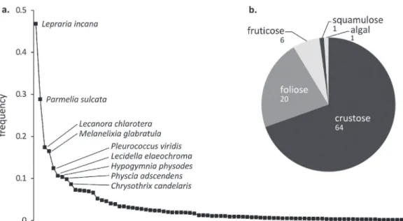
each study site are reported inTable 3. A total of 54 lichen

gen-era, distributed in 92 corticolous species, and an alga (Pleurococcus

viridis Ag.) were sampled (Fig. 3a). The most abundant species

were Lepraria incana (L.) Ach. (observed in 8 sites with a total fre-quency of 3.75), Parmelia sulcata Taylor (8 sites, frefre-quency of 2.31), Lecanora chlarotera Nyl. (7 sites, frequency of 1.32), and Melanelixia glabratula (Lamy) Sandler & Arup (6 sites, frequency of 1.05). Some species were found in only one site with a very low frequency (<0.005): e.g., Ramalina fastigiata (Pers.) Ach., Physcia leptalea (Ach.) DC, and Parmeliopsis ambigua (Wulfen) Nyl. Overall, the lichen species were distributed into 64 crustose, 20 foliose, 6 fruticose,

and one squamulose morphologies (Fig. 3b). The foliose/crustose

thallus ratios were from 0.05 to 1 and decreased as follows: CHS 35 < SP 11 < HET 54a < PM 72 < BEX < EPC 74 < EPC 63 < EPC 08.

Biological richness and abundance (sum of frequencies) showed a high heterogeneity among the study sites: from 13 to 35 species encountered by individual site and the abundances ranged between

Fig. 3. Lichen diversity found in the eight study sites: average abundance of each lichen species (a) and relative proportion of each type of morphology (b).

Table 4

Summary of main ecological, bioindication indices, and values of the six environmental variable fromWirth, 2010of each plotting area. study site ecological indices bioindication

indices

Wirth, 2010′_{s environmental indices (%)} lichen richness lichen abundance Shannon index

IAP LDV light temperature continentality humidity pH eutrophication

SP 11 35 2.85 4.43 241 57 55.8 52.3 44.8 26.3 32.6 43.2 HET 54a 33 3.77 4.30 263 75 62.7 51.1 42.9 21.8 37.6 47.5 EPC 74 30 3.60 4.27 227 72 76.4 50.1 45.8 18.5 36.5 46.0 PM 72 26 2.02 3.71 159 40 69.0 50.2 38.5 26.2 25.8 38.6 EPC 63 25 3.31 3.66 157 66 75.1 50.0 41.9 26.6 37.1 51.8 CHS 35 23 1.87 3.52 137 37 45.2 51.3 39.1 37.2 25.9 23.0 BEX 20 3.20 3.02 117 64 64.5 49.9 50.0 14.1 37.0 57.1 EPC 08 13 2.17 3.16 94 43 77.3 50.0 50.0 15.6 32.4 56.5

relatively low lichens abundance for a same range of richness (rich-ness/abundance ratio from 12.3 to 12.9) compared to the other sites (ratio from 6.0 to 8.8). The Shannon index, ranged between 3.02 and 4.43. It followed the lichen diversity values with the exception of

BEX site, which may be due to a higher abundance (Table 4).

The main lichen communities observed in the study sites were

commonly found in France (Coste, 2001; van van Haluwyn and

Lerond, 1993; van Haluwyn et al., 2009): Leprarion incanae Almborn 1948 (except in BEX and PM 72), including sciaphilous species (Lep-raria incana), and Lecanorion carpinae (Ochsn.) Barkm, 1958 (except in EPC 63 and CHS 35), including heliophilous, nitrophilous and toxitolerant species (such as Lecanora carpinea, Lecanora chlarotera, and Lecidella elaeochroma). Parmelion acetabuli Barkman 1958 was found in four sites (BEX, HET 54a, EPC 08, and PM 72), including Parmelia sulcata, Melanelixia glabratula, as well as Melanohalea exas-peratula and Physcia adscendens, mainly heliophilous and slightly neutrophilous and toxitolerant species. Other nitrophobous and poleophobous communities were found locally: Graphidion scriptae Oschner 1928 (with Arthonia, Graphis, Enterographa and Opegrapha; in HET 54a and CHS 35), Cladonion coniocraeae Duvigneaud ex James, Hawksworth & Rose, 1977 (with Cladonia fimbriata; in EPC 08 and PM 72), and Calicion viridis ˇCernh. & Hadaˇc 1944 (with Chrysothrix candelaris; in BEX).

The sampling procedure, including both hardwood and conifer

trees as far as possible (Table 1), attempted to reduce the tree bark

influence by limiting to only sample the main representative tree species in each site (i.e., fir in SP11, spruce in EPC 63, beech for HET 54a, oak in CHS 35, etc.), and thus, the lichen communities adapted

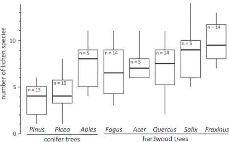
to these tree species. We collected lichen samples on a total of 21 different tree species, from 3 to 9 by site. Considering dominant

tree species (n ≥ 5,Fig. 4), lichen richness observed on hardwood

trees was usually greater compared to richness on conifers, except for Abies: p < 0.05 (Student test). Fraxinus was the tree species with the greater lichen richness (9.6 species on average). Also, the lichen communities found on deciduous trees (Lecanorion carpinae and Parmelion acetabuli associated with other foliose and fruti-cose species) differed from those on conifers (generally Leprarion incanae).

3.1.2. Bioindication indices

The highest IAP (>200) were found in HET 54a, SP 11, and EPC 74, while EPC 08 and BEX showed the lowest values (<120), following

a similar trend as lichen richness (Table 4). The different sampling

and/or calculation methods may limit the data comparison (Scerbo

et al., 1999). Lichen diversity values were also highest (>70) in HET 54a and EPC 74, but the lowest values (≤40) were for the two West-ern stations (CHS 35 and PM 72), following the lichen abundance trend.

3.1.3. Ecological features

For each lichen species, we studied ecological features through

six environmental parameters described byWirth (2010): light,

temperature, continentality, humidity, pH, and eutrophication. When ecological data were absent (i.e., for 25 species), we

used data from Nimis and Martellos (2008) database, as well

Fig. 4. Lichen diversity by tree-support species (n indicates the number of individuals for each tree genus). Smith et al., 2009; van Haluwyn and Lerond, 1993). An

aver-age ecological value of each parameter was calculated for each station based on individual value and frequency of each lichen species. To better homogenize the indices between these differ-ent references and to reduce the wide ranges (generally nine

levels are reported byWirth, 2010), we introduced a new scale

of three levels (e.g., xerophytic/mesophytic/hygrophytic species, acid/neutral/basic substrate pH, etc.). The results were expressed

using the frequency of each lichen species (Table 4).

The most important gradient were found for eutrophication (from low, i.e., CHS 35 and PM 72, to moderate eutrophic species, i.e., BEX and EPC 08) and light (with high proportions of helio-philous species, i.e., EPC 08, EPC 74, and EPC 63, and species with moderate light affinity, i.e., CHS 35 and SP 11). In contrast, mesophytic species were dominant indicating a low difference in temperature among sites. On overall, lichen species were, on aver-age, mostly acidophilic, xerophilic and moderately oceanic in all the stations.

3.2. Coupling ecological and biogeochemical approaches

To determine the resistance or sensitivity of each lichen species to metal atmospheric pollution, we performed multivariate sta-tistical analyses including the three diversity variables previously studied (lichen richness, lichen abundance, and Shannon index), the six ecological parameters mentioned above, the two bioindication indices (IAP and LDV), and metal bioaccumulation data measured in foliose lichen species (i.e., Xanthoria parietina, Parmelia sulcata, or Hypogymnia physodes) estimated using the sum of enrichment factors (EF) for 17 metals (Al, As, Cd, Co, Cr, Cs, Cu, Fe, Mn, Ni, Pb,

Sb, Sn, Sr, Ti, V, and Zn; seeAgnan et al. (2015)). A PCA was then

performed and the first two components (81% of the data variance)

were represented (Fig. 5).

The first component (45% of the data variance) was influenced by lichen abundance and LDV with negative scores. It was associated to lichen species living on basic bark and eutrophic, continental, and bright environments, as illustrated by EPC 74, BEX, HET 54a, and EPC 63 sites. The positive scores were characterized by hydrophilic species and metal EF data from bioaccumulation in lichen, influ-encing the two Western sites (CHS 35 and PM 72). The second component (36% of the data variance) grouped the two diversity indices (lichen richness and Shannon index), as well as IAP and lichen species living in warmer environments. The temperature could not explain this component due to the lack of ecological

con-trast in the study sites. This component distinguished SP 11 and HET 54a with positive scores, and EPC 08, and to a lesser extent BEX, with negative scores.

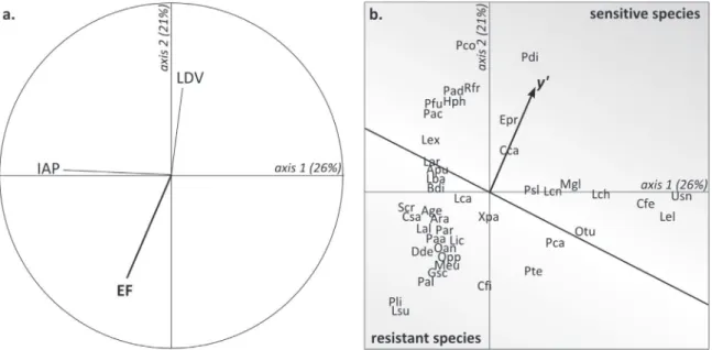
A CCA was performed on metal bioaccumulation data and

lichen species frequencies found for each study site (Fig. 6a,b).

This method was already used for lichen sensitivity to nitrogen by

Glavich and Geiser (2008). Only lichen species presented in at least two different study sites were included in the CCA. We added in

the analysis the sum of EF of the 17 metals previously cited (Agnan

et al., 2014) and the two bioindication indices (IAP and LDV). The IAP was explained by the first axis (26% of the data variance), while the second axis (21% of the data variance) evidenced an opposite

pattern between LDV and EF (Fig. 6a). Each lichen species was

repre-sented by a three letter code onFig. 6b (seeTable 5for the species

correspondence). Since IAP was a diversity index (Fig. 5), it was

proved difficult to classify the lichen species following the first axis. Using the EF position in the first plot as factor of metal pollution (Fig. 6a), however, we determined the degree of metal influence for each lichen species depending on the position of the species in the

second plot (Fig. 6b). To scale this influence, we applied a

geomet-ric rotation using EF as the new y axis (y’). The rotated coordinates allowed differentiation of sensitive vs resistant species based on the

EF values (i.e., projection on the EF gradient, y = 2.28 x;Fig. 6b). The

lowest and negative y’ indicated a resistant species to metal atmo-spheric pollution and the highest and positive y’ a sensitive species (Table 5). Given the range of y’ values of 3 (between −1.5 to +1.5), we determined three groups of identical ranges as follows: y’ < −0.5 for resistant species, −0.5 < y’ < 0.5 for intermediate species, y’ > 0.5 for sensitive species. The list of resistant species included various crustose lichens, while only two crustose species were present in the sensitive list (Pertusaria coccodes and Caloplaca ferruginea). Two foliose (Melanohalea exasperatula and Physcia tenella) and one fruti-cose (Cladonia fimbriata) species, however, were found as resistant species. The number of sites where each lichen species was present was given as confidence information of y’.

4. Discussion

4.1. Lichen diversity and communities

The diversity of corticose lichen species observed in the eight forest study sites was generally lower on coniferous trees

com-pared to hardwood trees (Fig. 4), confirming literature observations

Fig. 5. Principal component analysis (PCA) including ecological characteristics (normal), ecological indices (italic), bioindication indices (bold), and the sum of enrichment factors of 17 metals (EF, bold and italic).

Fig. 6. Canonical correspondence analysis based on frequency of the 43 main lichen species (presented in more than two different sites, with a three letter code, seeTable 4 for the species correspondence), bioindication (IAP and LDV) and bioaccumulation (sum of enrichment factors [EF] of 17 metals) indices for each study site.

these two types of trees with mostly sciaphilous communities on conifers and heliophilous species on hardwood trees (e.g., Leprarion incanae vs Lecanorion carpinae in EPC 74, respectively). Our sam-pling method in open areas bordering forests allowed therefore maximizing lichen diversity and communities: both sciaphilous and heliophilous lichens were found as dominant species (Lepraria

incana and Parmelia sulcata, respectively;Fig. 3).

Overall, the lichen diversity observed in the study sites was high. The number of lichen species was in the same range as those

observed in other European forests: e.g., in Italy (Giordani, 2007),

Slovenia (Poliˇcnik et al., 2008), or Portugal (Pinho et al., 2004);

the Shannon index, however, showed higher values compared to

other European and North American forested sites (Mulligan, 2009;

Peterson and McCune, 2001). But, this range was higher than in

boreal environments (Kuusinen, 1996), probably in relation to

spe-cific climate conditions in cold regions. Indeed, the diversity data from the literature are not always comparable since the sampling methods used can sometimes lead to discrepancies between the

observations (e.g.,Kuusinen and Siitonen, 1998; Selva, 1994).

Based on the indices ofNimis and Martellos (2008), 12% of the

overall taxa were pioneer species, with the maximum proportion for BEX and SP 11 (25 and 20%, respectively) and the minimum for CHS 35 (4%). In BEX, two common lichen species (Lecanora chlarotera and Lecidella elaeochroma) were responsible for 98% of the pioneer frequency, but these species can also be found in

non-pioneer environments (Pirintsos et al., 1995). The pioneer

fre-quency was not directly positively correlated with lichen richness (Table 4), as suggested bySelva (1994). This can be explained either by our sampling protocol in open field limiting forest, or by

inad-equateNimis and Martellos (2008)pioneer index applied in our

study sites.

Differences were, conversely, observed among study sites regarding ecological characteristics. For example, SP 11 and EPC 08 showed both nitrophilous and poleotolerant communities, while nitrophobous species were found in CHS 35 and HET 54a. This agreed with observations in atmospheric deposition sometimes different from modeled estimates, particularly under-estimated in the Pyrenees (SP 11) and over-estimated in the Armorican

Mas-Table 5

List of resistant, intermediate, and sensitive lichen species relative to atmospheric metal pollution based on a bioaccumulation–lichen diversity coupling method. y’ value indicates the new scale of lichen resistance/sensitivity to metals. The number of sites where each lichen species was present gives a confidence information of y’.

lichen species number of sites code y’

resistant species Lecanactis subabietina 3 Lsu −1.442

Pertusaria leioplaca 2 Pli −1.402

Pertusaria albescens 4 Pal −1.093

Graphis scripta 3 Gsc −0.919

Cladonia fimbriata 4 Cfi −0.893

Melanohalea exasperatula 2 Meu −0.854

Dendrographa decolorans 3 Dde −0.799

Ochrolechia pallescens subsp. parella 2 Opp −0.781

Ochrolechia androgyna 2 Oan −0.656

Pertusaria amara 3 Paa −0.620

Lepraria incana 8 Lic −0.615

Lecanora allophana 2 Lal −0.608

Physcia tenella 2 Pte −0.555

Calicium salicinum 2 Csa −0.551

Acrocordia gemmata 4 Age −0.537

Schismatomma cretaceum 2 Scr −0.525

Arthonia radiata 4 Ara −0.513

intermediate species Lecidella elaeochroma 4 Lel −0.494

Chrysothrix candelaris 7 Cca −0.482

Lecanora chlarotera 7 Lch −0.428

Melanelixia glabratula 6 Mgl −0.389

Lecanora conizaeoides 3 Lcn −0.284

Lecanora expallens 2 Lex −0.234

Parmelia sulcata 8 Psl −0.187

Lecanora argentata 4 Lar −0.021

Ochrolechia turneri 2 Otu −0.018

Amandinea punctata 5 Apu 0.066

Lecanora barkmaniana 2 Lba 0.080

Buellia disciformis 2 Bdi 0.124

Lecanora carpinea 3 Lca 0.170

Parmelina carporrhizans 2 Pca 0.204

Xanthoria parietina 5 Xpa 0.244

Phlyctis argena 4 Par 0.493

sensitive species Pleurosticta acetabulum 2 Pac 0.519

Caloplaca ferruginea 2 Cfe 0.524

Pseudevernia furfuracea 2 Pfu 0.590

Hypogymnia physodes 5 Hph 0.706

Evernia prunastri 6 Epr 0.732

Usneasp. 2 Usn 0.739

Physcia adscendens 4 Pad 0.771

Ramalina farinacea 4 Rfr 0.824

Pertusaria coccodes 3 Pco 1.256

Physconia distorta 2 Pdi 1.405

sif (CHS 35;Boutin et al., 2015;Pascaud et al., 2016). Even though

no obvious correlation was observed with lichen richness, lichen abundance, or foliose/crustose thallus ratio, lichen communities

agreed with the ecological features described byWirth (2010):

e.g., CHS 35 had a low percentage of eutrophic species, unlike EPC 08. These ecological observations were therefore a complementary description to assess environmental quality that cannot be illus-trated by lichen richness or abundance only.

Results of bioindication indices showed that IAP were largely

higher than data from French urban areas (Gombert et al., 2004),

and LDV were generally in the upper range compared to other forest

sites in Europe (Giordani, 2007; Pinho et al., 2004; Poliˇcnik et al.,

2008). These indices were closely related to lichen richness and

lichen abundance, respectively (Table 4), which was supported by

the PCA results (Fig. 5). This is most likely due to their

calcula-tion method: only frequencies were used in LDV whereas Qi (i.e., the number of companion species, largely influenced by lichen diversity) is considered in IAP. Thereby, the difference of results

between IAP and LDV, already observed byPoliˇcnik et al. (2008),

can be attributed to the difference between lichen richness and lichen abundance strongly highlighted with the Northwestern sites (PM 72 and CHS 35) and SP 11, showing a high number of lichen species weakly abundant. Each index was mainly influenced by one

principal component (Fig. 5): axis 1 for LDV (45% of the data

vari-ance) and axis 2 for IAP (36% of the data varivari-ance). Based on lichen

ecological features (Nimis and Martellos, 2008), the signs of

envi-ronmental alteration (e.g., acid or poor nutrient environment) were mainly influenced by the positive scores of the first component, i.e., opposed to the LDV. It is likely that IAP, and thus lichen diver-sity, were mostly driven by climate variable (temperature) despite a low gradient of temperature among lichen species. The sites PM 72 and CHS 35, both positively influenced by the first axis, may either reflect an environmental alteration (i.e., more acid conditions), or be driven by the continentality–humidity axis due to their location with Atlantic influence.

4.2. Resistance and sensitivity of lichen species to metal atmospheric pollution

As observed in the PCA (Fig. 5), the LDV was opposed to the sum

of metal enrichment factors in the axis 1 vs axis 2 plot. This implies that, in addition to the response toward the general alteration of environment, this index better responds to metal pollution as well. Indeed, the three lowest LDV were observed in CHS 35, PM 72, and EPC 08 (positive scores of the first axis of the PCA and negative scores of the second axis), that correspond to the highest EF and

The northeastern France is impacted by various activities (local industries, metallurgy, and mining), while both energy and metal-lurgy may explain such contamination in the northwestern France

(already observed in upper horizons;Hernandez et al., 2003). This

may be the dominant influence for CHS 35 and PM 72 in the PCA toward other environmental variables. Thus, it can be supposed that metal pollution affects more lichen abundance (illustrated by LDV) than lichen richness (IAP). This is in agreement with results fromJeran et al. (2002), who had previously observed that IAP was not a good index for metal pollution.

Based on the CCA, we evaluated the resistance or

sensitiv-ity of each lichen species to metal pollution (Fig. 6andTable 5).

Very few literature observations, however, allowed supporting our results: Cladonia fimbriata (present in 4 sites, y’ = −0.893) is a well-known species able to grow on cadmium, lead, and zinc enriched

substrates (Cuny et al., 2004; Tyler, 1989), whereas conversely,

Hypogymnia physodes (present in 5 sites, y’ = 0.706), is known as

a metal sensitive species, particularly for copper (Hauck and Zöller,

2003). To validate our results, we verified any correlations with

other pollutants: in both resistant and sensitive groups. There were both acidophilic (e.g., Graphis scripta, Pertusaria albescens, Pertusaria coccodes) and nitrophilic (Dendrographa decolorans, Physcia

adscen-dens, Physconia distorta;Gombert et al., 2004) species, as well as

both tolerant (Melanohalea exasperatula, Physcia adscendens) and sensitive (Ochrolechia pallescens, Lecanora allophana, Physconia

dis-torta;Wirth, 1991) to SO₂/NO₂pollution species. This implies that

we cannot attribute the y’ values to sulfur and nitrogen pollution influence, these elements being well known as major atmospheric pollutants. In this way, our method allowed correct evaluation of the influence of metal without other major disturbance. However,

organic pollutants also accumulated by lichens (Bajpai et al., 2010;

Harmens et al., 2013), were not investigated here. By applying the frequencies of studied species to these indices, and comparing to

the enrichment factors fromAgnan et al. (2015), we observed that

the four more polluted sites (i.e., HET 54a, EPC 08, CHS 35, and PM 72) as evidenced by bioindication, obtained negative scores (i.e., dominated by resistant lichen species), while several less contam-inated sites (e.g., EPC 63 and EPC 74) obtained positive values (i.e., dominated by sensitive lichen species).

These preliminary data need to be completed and compared with additional data from other European forest sites. Thus, it will be possible to determine the maximum exposure of metal pollu-tion without significant harmful effects (also called critical load) as

already done for nitrogen (Geiser et al., 2010).

5. Conclusions

This study aimed to evaluate the resistance or sensitivity of lichen species to atmospheric metal pollution. We performed eight lichen plottings in French and Swiss forested sites, and used different biomonitoring approaches (lichen richness, lichen abundances, lichen community description, ecological features, bioindication indices, as well as metal bioaccumulation) for a com-plete environmental description. Each method provided its own contribution to this investigation; similar results were demon-strated by lichen communities and ecological features. Ninety-two corticolous species were sampled, including 70% of crustose lichens. The abundance was higher on hardwood trees compared to conifers. The lichen diversity value (LDV) showed a better response to both ecological disturbances (largely influenced by light and nutrient conditions, such as eutrophication and pH) and metal pol-lution compared to the index of atmospheric purity (IAP).

Using a multivariate approach coupling frequencies of each lichen species and metal bioaccumulation data, we performed an innovative scale of resistance/sensitivity to metals for the 43 more

frequent lichen species, distinguishing sensitive, intermediate, and resistant species to metal pollution. To validate these results, we compared to the few data available in the literature, and checked any correlation with sensitivity to acid and nitrogen pollution. This approach constitutes a first insight into the investigation of resis-tance and sensitivity of lichen species to metals in open forested sites far from local pollution sources, which should be enhanced by results with data from other European forests in future researches.

Acknowledgements

This project benefited from financial support number 1062C0019 from ADEME (French Agency for Environment). The authors thank Clother Coste for his help in lichen determina-tion. Yannick Agnan was funded with ADEME fellowship. Thanks to four anonymous reviewers for their relevant comments that improved this manuscript.

References

Agnan, Y., Séjalon-Delmas, N., Probst, A., 2014.Origin and distribution of rare earth elements in various lichen and moss species over the last century in France. Sci. Total Environ. 487, 1–12.

Agnan, Y., Séjalon-Delmas, N., Claustres, A., Probst, A., 2015.Investigation of spatial and temporal metal atmospheric deposition in France through lichen and moss bioaccumulation over one century. Sci. Total Environ. 529, 285–296. Asta, J., Erhardt, W., Ferretti, M., Fornasier, F., Kirschbaum, U., Nimis, P.L., Purvis,

O.W., Pirintsos, S., Scheidegger, C., van Haluwyn, C., Wirth, V., 2002.Mapping lichen diversity as an indicator of environmental quality. In: Nimis, P.L., Scheidegger, C., Wolseley, P.A. (Eds.), Monitoring with Lichens – Monitoring Lichens. Kluwer/NATO Science Series, Dordrecht, pp. 273–279.

Bajpai, R., Upreti, D.K., Nayaka, S., Kumari, B., 2010.Biodiversity, bioaccumulation and physiological changes in lichens growing in the vicinity of coal-based thermal power plant of Raebareli district, north India. J. Hazard. Mater. 174, 429–436.

Bargagli, R., Nimis, P.L., 2002.Guidelines for the use of epiphytic lichens as biomonitors of atmospheric deposition of trace elements. In: Nimis, P.L., Scheidegger, C., Wolseley, P.A. (Eds.), Monitoring with Lichens – Monitoring Lichens, Earth and Environmental Sciences. Kluwer/NATO Science Series, Dordrecht, pp. 295–299.

Berge, E., Bartnicki, J., Olendrzynski, K., Tsyro, S.G., 1999.Long-term trends in emissions and transboundary transport of acidifying air pollution in Europe. J. Environ. Manage. 57, 31–50.

Bosch-Roig, P., Barca, D., Crisci, G.M., Lalli, C., 2013.Lichens as bioindicators of atmospheric heavy metal deposition in Valencia, Spain. J. Atm. Chem. 70, 373–388.

Boutin, M., Lamaze, T., Couvidat, F., Pornon, A., 2015.Subalpine Pyrenees received higher nitrogen deposition than predicted by EMEP and CHIMERE

chemistry-transport models. Sci. Rep. 5, 12942.

Clauzade, G., Roux, C., 1985.Likenoj de Okcidenta E ˘uropo. Ilustrita determinlibro. Société Botanique du Centre Ouest, Royan.

Conti, M.E., Cecchetti, G., 2001.Biological monitoring: lichens as bioindicators of air pollution assessment – a review. Environ. Pollut. 114, 471–492. Conti, M.E., Finoia, M.G., Bocca, B., Mele, G., Alimonti, A., Pino, A., 2011.

Atmospheric background trace elements deposition in Tierra del Fuego region (Patagonia, Argentina), using transplanted Usnea barbata lichens. Environ. Monit. Assess. 184, 527–538.

Coste, C., 2001.Flore et végétation lichéniques épiphytes du parc de Lostange (France, Tarn). Cryptogam. Mycol. 22, 209–223.

Cuny, D., Denayer, F.-O., de Foucault, B., Schumacker, R., Colein, P., van Haluwyn, C., 2004.Patterns of metal soil contamination and changes in terrestrial cryptogamic communities. Environ. Pollut. 129, 289–297.

Daillant, O., Moreau, P.-A., Corriol, G., Agnello, G., Courtecuisse, R., 2007.Inventaire Des Champignons Et Des Lichens Sur 30 Placettes RENECOFOR 2007. Deruelle, S., Garcia Schaeffer, F., 1983.Les lichens bioindicateurs de la pollution

atmospherique dans la region parisienne. Cryptogam.: Bryol. Lichenol. 4, 47–64.

Dobson, F., 2011.Lichens: an Illustrated Guide to the British and Irish Species. Richmond Pub., Slough, England.

Dray, S., Dufour, A.-B., 2007.The ade4 package: implementing the duality diagram for ecologists. J. Stat. Softw. 22, 1–20.

EN 16413, 2014.Ambient Air. Biomonitoring with Lichens. Assessing Epiphytic Lichen Diversity. Comité Européen de Normalisation.

Ellis, C.J., 2012.Lichen epiphyte diversity: a species, community and trait-based review. Perspect. Plant Ecol. Evol. Syst. 14, 131–152.

Gandois, L., Probst, A., Dumat, C., 2010a.Modelling trace metal extractability and solubility in French forest soils by using soil properties. Eur. J. Soil Sci. 61, 271–286.

Gandois, L., Tipping, E., Dumat, C., Probst, A., 2010b.Canopy influence on trace metal atmospheric inputs on forest ecosystems: speciation in throughfall. Atmos. Environ. 44, 824–833.

Gauslaa, Y., 1995.The Lobarion, an epiphytic community of ancient forests threatened by acid rain. Lichenologist 27, 59–76.

Geiser, L.H., Neitlich, P.N., 2007.Air pollution and climate gradients in western Oregon and Washington indicated by epiphytic macrolichens. Environ. Pollut. 145, 203–218.

Geiser, L.H., Jovan, S.E., Glavich, D.A., Porter, M.K., 2010.Lichen-based critical loads for atmospheric nitrogen deposition in Western Oregon and Washington Forests, USA. Environ. Pollut. 158, 2412–2421.

Giordani, P., Calatayud, V., Stofer, S., Granke, O., 2011.Epiphytic lichen diversity in relation to atmospheric depsition. In: Fischer, R., Lorenz, M. (Eds.), Foreest Condition in Europe, 2011 Technical Report of ICP Forest and FutMon, Work R Eport of the In Stitute for World Forestry 2011/1. Hamburg, Germany, pp. 128–143.

Giordani, P., Brunialti, G., Bacaro, G., Nascimbene, J., 2012.Functional traits of epiphytic lichens as potential indicators of environmental conditions in forest ecosystems. Ecol. Indic. 18, 413–420.

Giordani, P., 2006.Variables influencing the distribution of epiphytic lichens in heterogeneous areas: a case study for Liguria, NW Italy. J. Veg. Sci. 17, 195–206. Giordani, P., 2007.Is the diversity of epiphytic lichens a reliable indicator of air

pollution? A case study from Italy. Environ. Pollut. 146, 317–323.

Glavich, D.A., Geiser, L.H., 2008.Potential approaches to developing lichen-based critical loads and levels for nitrogen, sulfur and metal-containing atmospheric pollutants in North America. Bryologist 111, 638–649.

Gombert, S., Asta, J., Seaward, M.R.D., 2004.Assessment of lichen diversity by index of atmospheric purity (IAP), index of human impact (IHI) and other

environmental factors in an urban area (Grenoble, southeast France). Sci. Total Environ. 324, 183–199.

Harmens, H., Foan, L., Simon, V., Mills, G., 2013.Terrestrial mosses as biomonitors of atmospheric POPs pollution: a review. Environ. Pollut. 173, 245–254. Hauck, M., Zöller, T., 2003.Copper sensitivity of soredia of the epiphytic lichen

Hypogymnia physodes. Lichenologist 35, 271–274.

Hawksworth, D.L., Rose, F., 1970.Qualitative scale for estimating sulphur dioxide air pollution in Engand and Wales using epiphytic lichens. Nature 227, 145–148.

Hernandez, L., Probst, A., Probst, J.L., Ulrich, E., 2003.Heavy metal distribution in some French forest soils: evidence for atmospheric contamination. Sci. Total Environ. 312, 195–219.

Hissler, C., Stille, P., Krein, A., Geagea, M.L., Perrone, T., Probst, J.L., Hoffmann, L., 2008.Identifying the origins of local atmospheric deposition in the steel industry basin of Luxembourg using the chemical and isotopic composition of the lichen Xanthoria parietina. Sci. Total Environ. 405, 338–344.

Jeran, Z., Ja´cimovi´c, R., Batiˇc, F., Mavsar, R., 2002.Lichens as integrating air pollution monitors. Environ. Pollut. 120, 107–113.

Kuusinen, M., Siitonen, J., 1998.Epiphytic lichen diversity in old-growth and managed Picea abies stands in Southern Finland. J. Veg. Sci. 9, 283–292. Kuusinen, M., 1996.Epiphyte flora and diversity on basal trunks of six old-growth

forest tree species in Southern and middle boreal Finland. Lichenologist 28, 443–463.

Lallemant, R., Joslain, H., Houssay, I., Cyprien, A.-L., 1996.The Use of Lichens for Estimating Ammonia Air Pollution in Western France, Report to the Upres Biocatlalyse. Université de Nantes, Nantes.

LeBlanc, S.C.F., Sloover, J.D., 1970.Relation between industrialization and the distribution and growth of epiphytic lichens and mosses in Montreal. Can. J. Bot. 48, 1485–1496.

Loppi, S., Frati, L., Paoli, L., Bigagli, V., Rossetti, C., Bruscoli, C., Corsini, A., 2004. Biodiversity of epiphytic lichens and heavy metal contents of Flavoparmelia caperata thalli as indicators of temporal variations of air pollution in the town of Montecatini Terme (central Italy). Sci. Total Environ. 326, 113–122. Moreau, P.-A., Daillant, O., Corriol, G., Gueidan, C., Courtecuisse, R., 2002.Inventaire

des champignons supérieurs et des lichens sur 12 placettes du réseau et dans un site atelier de L’INRA/GIP ECOFOR: résultats d’un projet pilote (1996–1998). Office national des forêts, Dept. recherche et développement, Fontainebleau.

Mulligan, L., 2009.An Assessment of Epiphytic Lichens, Lichen Diversity and Environmental Quality in the Semi-Natural Woodlands of Knocksink Wood Nature Reserve, Enniskerry, County Wicklow. (Master). Dublin Institute of Technology, Dublin.

Nimis, P.L., Martellos, S., 2008. ITALIC − The Information System on Italian Lichens. Version 4.0. University of Trieste, Dept. of Biology, IN4.0/1http://dbiodbs.univ. trieste.it/.

Nylander, W., 1866.Les lichens du jardin du Luxembourg. Bull. Soc. Bot. France 13, 364–372.

Pascaud, A., Sauvage, S., Coddeville, P., Nicolas, M., Croisé, L., Mezdour, A., Probst, A., 2016. Long-term trends in atmospheric deposition across France: drivers, forecasts and impacts. Atmos. Environ.,http://dx.doi.org/10.1016/j.atmosenv. 2016.05.019(In press)http://www.sciencedirect.com/science/article/pii/ S1352231016303600.

Peterson, E.B., McCune, B., 2001.Diversity and succession of epiphytic macrolichen communities in low-elevation managed conifer forests in Western Oregon. J. Veg. Sci. 12, 511–524.

Piervittori, R., Usai, L., Alessio, F., Maffei, M., 1997.The effect of simulated acid rain on surface morphology and n-alkane composition of Pseudevernia furfuracea. Lichenologist 29, 191–198.

Pinho, P., Augusto, S., Branquinho, C., Bio, A., Pereira, M.J., Soares, A., Catarino, F., 2004.Mapping lichen diversity as a first step for air quality assessment. J. Atmos. Chem. 49, 377–389.

Pirintsos, S.A., Diamantopoulos, J., Stamou, G.P., 1995.Analysis of the distribution of epiphytic lichens within homogeneousFagus sylvatica stands along an altitudinal gradient (Mount Olympos, Greece). Vegetation 116, 33–40. Poliˇcnik, H., Simonˇciˇc, P., Batiˇc, F., 2008.Monitoring air quality with lichens: a

comparison between mapping in forest sites and in open areas. Environ. Pollut. 151, 395–400.

Roux, C., 2012.Liste des lichens et champignons lichénicoles de France. Bull. Soc. linn. Provence.

Scerbo, R., Possenti, L., Lampugnani, L., Ristori, T., Barale, R., Barghigiani, C., 1999. Lichen (Xanthoria parietina) biomonitoring of trace element contamination and air quality assessment in Livorno Province (Tuscany, Italy). Sci. Total Environ. 241, 91–106.

Schulze, E.-D., Lange, O.L., Oren, R. (Eds.), 1989.Ecological Studies. Springer, Berlin, Heidelberg.

Selva, S.B., 1994.Lichen diversity and stand continuity in the Northern hardwoods and spruce-fir forests of Northern New England and Western New Brunswick. Bryologist 97, 424–429.

Shukla, V., Upreti, D.K., Bajpai, R., 2014.Lichens to Biomonitor the Environment. Springer, India, New Delhi.

Sigal, L.L., Johnston, J.W., 1986.Effects of acidic rain and ozone on nitrogen fixation and photosynthesis in the lichen Lobaria pulmonaria (L.) Hoffm. Environ. Exp. Bot. 26, 59–64.

Smith, C.W., Aptroot, A., Coppins, B.J., Fletcher, A., Gilbert, O.L., James, P.W., Wolseley, P.A. (Eds.), 2009,2nd ed. British Lichen Society, London. Szczepaniak, K., Biziuk, M., 2003.Aspects of the biomonitoring studies using

mosses and lichens as indicators of metal pollution. Environ. Res. 93, 221–230. Tyler, G., 1989.Uptake, retention and toxicity of heavy metals in lichens. Water Air

Soil Pollut. 47, 321–333.

Vonarb, C., Mueller, C., Ammann, K., Brunold, C., 1990.Lichen physiology and air pollution. II-Statistical analysis of the correlation between SO2, NO2, NO and O3, and chlorophyll content, net photosynthesis, sulfate uptake and protein synthesis of Parmelia sulcata Taylor. New Phytol. 115, 431–437.

Wirth, V., 1991.Zeigerwerte von flechten. Scr. Geobot. 18, 215–237. Wirth, V., 2010.Ökologische Zeigerwerte von Flechten −erweiterte und

aktualisierte Fassung. Herzogia 23, 229–248.

van Haluwyn, C., Lerond, M., 1993.Guide Des Lichens. Lechevalier, Paris. van Haluwyn, C.V., Asta, J., Gavériaux, J.-P., 2009.Guide des lichens de France: