O
pen
A
rchive
T
OULOUSE
A
rchive
O
uverte (
OATAO
)
OATAO is an open access repository that collects the work of Toulouse researchers and makes it freely available over the web where possible.
This is an author-deposited version published in : http://oatao.univ-toulouse.fr/
Eprints ID : 19043
The contribution was presented at KES 2017 :
http://kes2017.kesinternational.org/
To link to this article URL :
https://doi.org/10.1016/j.procs.2017.08.116
To cite this version : Mothe, Josiane and Washha, Mahdi Predicting the Best System Parameter Configuration: the (Per Parameter Learning) PPL method. (2017) In: 21st International Conference on Knowledge-Based and Intelligent Information & Engineering Systems (KES 2017), 6 September 2017 - 8 September 2017 (Marseille, France).
Any correspondence concerning this service should be sent to the repository administrator: [email protected]
International Conference on Knowledge Based and Intelligent Information and Engineering
Systems, KES2017, 2017, Marseille, France
Predicting the Best System Parameter Configuration:
the (Per Parameter Learning) PPL method
Josiane Mothe
a,b,∗, Mahdi Washha
1,baESPE, Universit´e Jean-Jaur`es, Universit´e de Toulouse, Toulouse, France
bIRIT, Institut de Recherche en Informatique de Toulouse, UMR5505 CNRS, Toulouse, France cUniversit´e Paul Sabatier, Universit´e de Toulouse, Toulouse, France
Abstract
Search engines aim at delivering the most relevant information whatever the query is. To proceed, search engines employ various modules (indexing, matching, ranking), each of these modules having different variants (e.g. different stemmers, different retrieval models or weighting functions). The international evaluation campaigns in information retrieval such as TREC revealed system variability which makes it impossible to find a single system that would be the best for any of the queries.
While some approaches aim at optimizing the system parameters to improve the system effectiveness in average over a set of queries, in this paper we consider a different approach that aims at optimizing the system configuration on a per-query basis. Our method learns the configuration models in a training phase and then explores the system feature space and decides what should be the system configuration for any new query.
The experimental results draw significant conclusions: (i) Predicting the best value for each system feature separately is more effective than predicting the best predefined system configuration; (ii) the method predicts successfully the optimal or most optimal system configurations for unseen queries; (iii) the mean average precision (MAP) of the system configurations predicted by our approach is much higher than the MAP of the best unique system.
c
2016 The Authors. Published by Elsevier B.V. Peer-review under responsibility of KES International.
Keywords: Information systems, Information retrieval, machine learning, best system configuration, optimization of effectiveness, system parameters
1. System variability and best system parameters
Search engines aim at delivering the most relevant information according to an information need, a user expresses through a query. Offline, search engines index documents in order to associate key-words to documents; online they match the query terms with the document indexes and display the documents according to their scores. At any of these steps (indexing, matching, ranking), many parameters are implied. For example, Terrier platform (http://terrier.org/)
∗Corresponding author: Pr. Josiane Mothe Tel.: +33-5 61 55 64 44
implements various indexing (e.g. various stemmers) and matching methods (e.g. BM25, language modeling, each in turn having various inner parameters).
The international evaluation campaigns in information retrieval (IR) such as TREC revealed that system variability is high7,3. System variability refers to the fact that system S1 performs well on query Q1 but badly on query Q2, while system S2 performs the opposite. This fact is a major difficulty in defining the best system configuration, that is the best system parameter values, that would fit for any query.
Because of the system variability, optimizing the system configuration for the all set of queries leads to a sub-optimal solution. Linking directly the input query with the corresponding best system would be an alternative solution to approach the performance variability2. However, this approach fits only in the case of queries that are known in advance such as repeated queries, which is not the general case. In this paper, we rather learn the system configuration that best fit a given query based on query features and system performance. In this paper, a system configuration refers to the set of specific modules and parameters used in the system. In the experiment part, we do not focus on the inner system parameters such as k1, k3 or b in BM25 for example, but rather on high level features such as the retrieval model used as for example, BM25, LM, ... although the same approach could have been applied to inner system parameters.
Query-based approaches have been developed in the literature. For example, in query difficulty prediction, query features are used in order to decide whether the system is going to fail or succeed processing a query4. Linguistic-based as well as statistically-Linguistic-based features have been proposed; some being pre-retrieval features and other post-retrieval. Pre-retrieval features are computed from the query or from the collection (e.g. Inverse Document Frequency or average number of senses of the query terms according to WordNet9), while post-retrieval features need the query to be processed first by a system and then use some statistics or characteristics from the retrieved documents (e.g. standard deviation between the top retrieved documents13).
Selective query expansion is another example of query-based decision. Selective query expansion is another ex-ample of query-based decision. The system automatically decides if the query will benefit from query expansion or not based on query features1after training a decision function.
On the other hand, learning to rank learn a ranking function by which the document ranking is optimized12. As
opposed to the two previous applications (predicting query difficulty and selective query expansion where examples are queries represented by their features and performance), the training data in learning to rank is composed of query-documents pairs represented by feature vectors and a relevance judgment of the document for the query16,8.
Although somehow similar5, the problem that we tackle differ from learning to rank as usually applied in IR as we aim at learning the best value for the system parameters in order to predict the best system configuration that should be used for any new query. Thus we do not directly optimize the document ordering as learning to rank approaches do.
Other related work aims at optimizing effectiveness based on query features. Plachouras et al. predict the optimal weighting functions (document and term weighting) from a set of candidate functions on a per-query basis11. The authors first cluster the queries according to their features and then associate the best weighting function to the cluster. This method handles the unseen queries by clustering them as a preliminary step, then the learned weighting function predicts the weights according to which cluster the unseen query belongs to.
Goswami et al. developed a method to learn an IR function on a particular collection without relevance judgments by transferring knowledge from a source domain collection, where the relevance judgments are known, to a target domain collection. The normalized document frequency and term frequency, represented in grids, are used only in transferring the information between the domains6. Wu et al. use post-retrieval features in order to predict the performance of data fusion algorithms15. In their approach, the learning phase is based on multiple regression models that are based on fusing different algorithms where four different post-retrieval features are used in the learning phase. Our approach is different since it does not aim at fusing various results, but rather select the best value for the system parameters that fits a given query.
This paper presents a novel method by which the best value of each system parameters is predicted for unseen queries. It optimizes a particular effectiveness retrieval measurement (e.g. Average Precision) chosen in the learning phase. Rather than learning a classification model on a set of predefined systems, our method learns a classification model for each system parameter; for this reason we named it PPL (Per Parameter Learning). Doing so, the space used for training is larger. Indeed, if the learning function was trained on predefined systems, one of those predefined
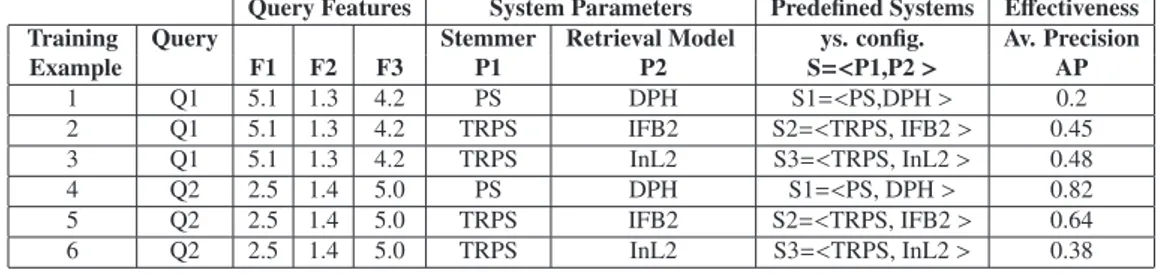
Table 1. Candidate training examples for two queries which are used in training two classifiers that will predict the best values of the system parameters individually (P1 and P2) and will optimize the average precision.
Query Features System Parameters Predefined Systems Effectiveness Training Query Stemmer Retrieval Model ys. config. Av. Precision Example F1 F2 F3 P1 P2 S=<P1,P2 > AP 1 Q1 5.1 1.3 4.2 PS DPH S1=<PS,DPH > 0.2 2 Q1 5.1 1.3 4.2 TRPS IFB2 S2=<TRPS, IFB2 > 0.45 3 Q1 5.1 1.3 4.2 TRPS InL2 S3=<TRPS, InL2 > 0.48 4 Q2 2.5 1.4 5.0 PS DPH S1=<PS, DPH > 0.82 5 Q2 2.5 1.4 5.0 TRPS IFB2 S2=<TRPS, IFB2 > 0.64 6 Q2 2.5 1.4 5.0 TRPS InL2 S3=<TRPS, InL2 > 0.38
systems would be chosen at the prediction level. Since the learning function is trained at the parameter level, it will predict each parameter value individually which could result in a configuration that was not in the set of predefined systems. Although the detailed analysis of this feature is out of the topic of this paper, we do believe this can be one of its advantage.
The rest of the paper is organized as follows: Section2describes our PPL method in details. Section3depicts the experimental setup. The experimental results along with discussion are reported in Section4. Section5concludes the paper.
2. Learning the best system parameter - PPL principles
The objective of the PPL method is to predict the best value for a set of parameters in order to optimize retrieval effectiveness. In this section, we first present an illustrative example; we then detail the method.
2.1. Textbook case
We adopt the data shown in Table1, as an illustrative example. Each row is a candidate training example; we will see later on that not all the candidates are used in the training phase. A candidate training example consists of query features, system parameters which define a system configuration, and effectiveness measurement; the latter been used as the label during training not as a feature of the model. In our example we use three query features (F1, F2, and F3); such features could be any query features but we will see in section3that in our experiments we use pre- and post-retrieval query features from query difficulty prediction literature. System parameters control the IR system behavior and each parameter may have one or many possible values. In the given example, we consider two parameters: the stemmer algorithm (P1) and the retrieval model (P2). For the parameter P1, PS and TRPS are the two possible values, and DPH, IFB2, and InL2 are the three possible values for P2. In the experiments, we use more parameters and more values for each parameter.
A configuration consists of the set of parameters along with their values; a configuration is denoted as S=<P1,P2> in the example. The candidate training examples are produced using predefined configurations. According to the possible values of the P1 and P2 parameters, 2x3, six configurations could be generated. However, when the number of parameters and values per parameters is high this is not possible to run all the possible configurations. For this reason, we generate a few configurations only. In the example, we generate three configurations only which correspond to what we call predefined systems (S1, S2, and S3). The training queries, Q1 and Q2, are then run over the predefined systems using a document collection for which the relevant documents are assumed to be known for those queries (named Qrels in TREC). It is thus possible to calculate for each query and each predefined system its effectiveness. We consider Average Precision (AP) as the effectiveness measure in the example. The full candidate training examples are presented in Table1.
None of the single predefined system can optimize AP for both Q1 and Q2. Therefore, to make the prediction function general enough, a possible solution could be to learn a function that predicts a predefined system maximizing AP based on query features; it could then work for any new query. The trivial and straightforward solution could be to learn a single function to predict the most suited predefined system which is S3 for Q1 (and thus for queries similar to Q1) and S1 for Q2. However, this solution is not optimal for unseen queries since the prediction models will be
restricted to the predefined systems. Indeed, in the evaluation section, we will show empirically that PPL is indeed much more effective than this trivial solution.
To solve this issue, rather than learning the best predefined system, we learn several functions, one per parameter. In the textbook case, we will learn two prediction functions, one for P1 and the other for P2.
When learning a parameter (e.g. P1), training examples are represented by the query features; the class to learn is the parameter value. Thus, when learning P1, the training examples will be limited to the 2nd, 3rd, 4th (query features) and 5th columns (class label). Moreover, since the function aims at optimizing AP, we cannot keep all the candidate training examples because some correspond to weak AP. We rather keep only the training examples for which AP is high enough. In our textbook case, let us say that we keep only the best AP for each query; we will keep two training examples from the candidates presented in Table1: the 3rd example (best AP for Q1) and the 4th example (best AP for Q2). In these two training examples we will thus consider 2 values for P1 (TRPS and PS) and 2 values for P2 (InL2 and DPH). For an unseen query, based on the query features, the functions will decide the best value for each parameter; that makes 4 possible configurations for prediction even if we learned only on two predefined systems. The number of training examples per query we select is an input for our method (in the used textbook case we set this value to 1).
To go beyond the textbook case, the next sections present in details the main steps of the PPL method, starting from pre-processing, passing over building the feature vector space, the training phase, and ending with predicting system parameter values for unseen query.
The PPL method input consists of: a document collection, a set of training queries along with their features, a set of system parameters (e.g. stemmer algorithm, retrieval model) for which the prediction functions are built, the number of best system configurations that will be chosen per query, and the effectiveness retrieval measure (e.g. AP, P@10). The output of the algorithm is a set of trained prediction functions where each function corresponds to a system parameter.
2.2. Step 1 Pre-processing: Corpus indexing, Generation of the runs associated with chosen system configurations, and Evaluation.
The document collection D is first indexed. Indexing is costly, thus it can be decided it is not a system parameter to be learned, but rather that it is set once for all. On the other hand, Terrier platform that we used in the experimental part implements several stemmers such as Porter Stemmer (PS), English Snowball Stemmer(ESS); thus in our experiments, we consider the stemmer algorithm as a system parameter to be learned.
After indexing, the next step is to generate the set of K system configurations including the various values of the considered parameters in P. If all the possible configurations were generated, the chance of getting the best prediction would be increased. However, in practice, it is time consuming to do so (if not impossible for continuous parameters that can take their values in the range of integer or even real numbers). To solve this issue we generate what we think is a relatively high number of configurations by considering various values for each parameter and combining them (see Table2). They are the predefined systems.
We then run these system configurations over each learning query q∈Qtraining. The retrieval effectiveness of the
generated configurations is measured for each learning query, using a particular measure M (e.g. AP). This process results in an evaluation array, E, where the rows correspond to training queries while the columns correspond to the system configurations with its effectiveness. This array comprise the candidate training examples.
2.3. Step 2: Selecting the best system configurations and building the feature vector space
Once the generated system configurations have been evaluated for each query using the performance measure M, the system configurations are sorted out in descending order of their performance, rt, and this for each query taken
independently. Then, still on a per query basis, the first N top system configurations are selected, resulting in a reduced evaluation array, ENwhich contains the selected training examples for the considered parameter. The motivation be-hind this is that for the same query, several system configurations may have the same or close effectiveness. Therefore, considering the top N system configurations in the learning phase may increase the accuracy of our prediction model. The number of feature vector spaces that is built equals to the number of the system parameters in P. The size of each feature vector space depends on the number of training queries, number of top system configurations (N), and the
number of the query features. A feature vector space vs for a parameter p in P consists in the training query features
Fqplus the corresponding value of p in EN, which will act as the class label.
2.4. Step 3: Training
The purpose of this step is to learn a classification function, y, for each system parameter in P, using the feature vector spaces from step 2. The resulting classification functions should be able to map query features to a set of best values for each parameter. The possible predicted values for a system parameter are the distinct values of the class labels in the corresponding feature vector space.
2.5. Step 4: Testing
For an unseen query, the value of each system parameter is predicted on the basis of the query features Fq. The
produced feature vector is passed over each trained system parameter model to determine the system configuration to be used, in the form of S =< p1, ...,pj>.
3. Experimental Setup
3.1. Topics and query features
We used the TREC disk4 & 5 minus the Congressional Record (http://trec.nist.gov/data/docs eng.html) collection in our experiments. It comprises a document collection of about half a million documents, a set of topics, and relevance assessments. We selected the 100 topics from TREC7 and TREC8 for which we considered the title part as the query to be submitted to the system configurations.
We represent the queries in terms of features. These features come from the query difficulty prediction literature4
; this paper does not add any contribution in this area but only use variations of existing features. 30 query features have been used in the query representation. We use pre- and post-retrieval features. Pre-retrieval can be calculated before the query is submitted to any system while post-retrieval ones need to evaluate the query.
We use four query difficultly predictors from the literature:
WordNet sense number10. This predictor is pre-retrieval that measures the ambiguity of the query. It is calculated
as the average number of query term senses in WordNet. For the query q, is is defined as:
W NS(q) = 1 nq nq X t=1 senset (1)
where nqis the number of terms in the query q, and sensetrepresents the number of WordNet synsets for the query
term t.
Inverse Document Frequency (IDF). It is also a pre-retrieval feature. It measures whether a term is rare or common in the corpus. It is defined as the average query term IDF over the query terms as follows:
IDF(q) = 1 nq nq X t=1 log10 N Nt+1 (2) where N is the total number of documents in the collection, and Nt the number of documents containing the query
term t.
The standard deviation (STD). It has been used as a post-retrieval query difficulty predictor and measures the degree of variation from the average of the scores of the retrieved document list. It is thus a variant of NQC14, without standardization. For a query q and the first n retrieved documents, the STD is calculated by the formula:
S T D(q) = (1 nq nq X i=1 (score(Diq) − 1 nq nq X j=1 score(Dqj))2) 1 2 (3)
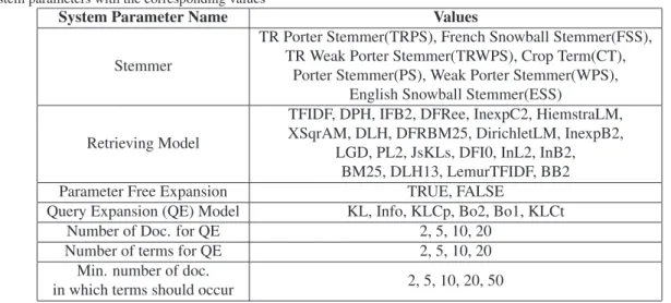
Table 2. System parameters with the corresponding values
System Parameter Name Values
Stemmer
TR Porter Stemmer(TRPS), French Snowball Stemmer(FSS), TR Weak Porter Stemmer(TRWPS), Crop Term(CT),
Porter Stemmer(PS), Weak Porter Stemmer(WPS), English Snowball Stemmer(ESS)
Retrieving Model
TFIDF, DPH, IFB2, DFRee, InexpC2, HiemstraLM, XSqrAM, DLH, DFRBM25, DirichletLM, InexpB2,
LGD, PL2, JsKLs, DFI0, InL2, InB2, BM25, DLH13, LemurTFIDF, BB2 Parameter Free Expansion TRUE, FALSE
Query Expansion (QE) Model KL, Info, KLCp, Bo2, Bo1, KLCt Number of Doc. for QE 2, 5, 10, 20
Number of terms for QE 2, 5, 10, 20 Min. number of doc.
in which terms should occur 2, 5, 10, 20, 50
where score(Di
q) represents the score of the ithretrieved document for the query q.
Query Feedback (QF)17. QF is a post-retrieval feature; it is calculated from two document lists and their overlap.
The first list is obtained when the initial query is used while the second list is obtained after expanding the query. The overlap represents the number of documents that are in common in the two lists. Lists can be cut-off at various levels considering the top x retrieved documents. In order to obtain a measurement between 0 and 1, the overlap is normalized by dividing it by x.
From these four basic predictors, we calculated a total of 30 features which are described below.
• Terms ambiguity features : six features as a variation of WNS : the maximum, average and sum of the number of senses of query terms. The characteristics are calculated for both the original short query (as defined by the TREC topic title), and the long query (as defined by the TREC topic title and description).
• Words discrimination: hight variant of IDF : the minimum, maximum, average, and sum of the IDF of the query terms. Like for Terms ambiguity, IDF variants are calculated for both the short and long queries.
• Homogeneity of document lists: variants of STD. We consider the STD value of the STD for the list of documents taken from the short query, the long query, and their difference.
• Document list divergence: variants of QF, considering combinations between the various lists for the short query and the expanded query using Bo2 algorithm; 4 different cutting levels are used (5, 10, 50, 100).
• Pre/Post-retrieval combinations: we also consider two combinations of precious features: the product of WNS using the short query and STD; the product of IDF by STD.
3.2. Systems
IR systems are controlled by various parameters. Terrier platform (http://terrier.org/) has been used since it imple-ments the most recent indexing, retrieving, and query expansion models available in the literature. Table2describes the system parameters with their corresponding possible values we use in our experiments; the details can be found on the platform web site. From these parameters values, we generated K=82, 627 system configurations.
TREC provides the relevance assessments which were used to compute system effectiveness. We choose AP as a measure of effectiveness.
3.3. Classifiers
Support vector machine (SVM) has been used in learning each IR system parameter. The kernel trick methods are applicable in the SVM learning algorithm. In this study, we used three kinds of kernels in order to compare them: (i) Radial Bias Function (RBF); (ii) Polynomial; (iii) Sigmoid. These kernels are controlled by various parameters; we
study only the gamma parameter value for both the RBF and Sigmoid kernels, and the polynomial degree parameter for the Polynomial kernel. The best value of the kernel parameters were determined as follows:
• A 10-folds cross validation was carried out using the three kernel methods for each IR system parameter consid-ered individually using different values, 1 to 5 for the polynomial degree parameter, and 1 to 10 for the gamma parameter.
• Then, the best kernel method with its best kernel parameter value was chosen, for each individual system parameter, according to the best accuracy through the cross validation experiments.
Table 3. Best kernel method with its parameter (polynomial degree, gamma) values for each system parameter for several values of N - top systems 1, 5, 10, and 20.
System Param N=1 N=5 N=10 N=20
Stemmer RBF,gamma=1 poly,deg=3 RBF,gamma=1 RBF,gamma=1
Retrieving model RBF,gamma=1 RBF,gamma=1 RBF,gamma=1 RBF,gamma=1
Parameter Free expansion RBF,gamma=1 RBF,gamma=1 RBF,gamma=1 RBF,gamma=1
Query Expansion (QE) Model poly,deg=2 RBF,gamma=1 poly,deg=1 poly,deg=3
Number of Documents for QE RBF,gamma=1 poly,deg=2 RBF,gamma=1 RBF,gamma=1
Number of terms for QE RBF,gamma=1 poly,deg=5 poly,deg=3 RBF,gamma=1
Minimum Number of documents RBF,gamma=1 RBF,gamma=1 RBF,gamma=1 RBF,gamma=1
Table3shows the best kernel method name with the best gamma and polynomial degree value for each considered IR system parameter, using different numbers of top predefined systems (N). The dominant kernel type is the RBF with gamma value of 1. One possible reason is that query features follow a Gaussian distribution with respect to the considered system parameter.
4. Results and Discussions
We evaluate the PPL method using 10-folds cross validation. Since we consider seven IR parameters, seven SVM classifiers are required to predict the system parameter values (after training).
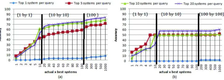
Fig. 1. Cross validation accuracy (a) when the individual system parameters are learned individually (b) when the predefined system is learned. Both consider AP as the effectiveness measure and various number of top systems in the training (1, 5, 10, and 20 system configurations per query) reported as different curves. The accuracy (Y-Axis) of the prediction is computed over a different number of actual best systems for each query, from 1 to 1000 with a changing scale which is marked-up by vertical black lines (X-Axis). The accuracy results from an average over queries and over the various draws resulting from 10-folds cross-validation principle.
Figure1(a) shows the accuracy of the prediction according to the number of top systems (N) used in the training phase. For any of the N top system curves, PPL has selected the N top system configurations for each query, identi-fying the selected training examples from the candidate ones. After training, the testing queries have been proceeded by the learned classifiers. The accuracy has been calculated as follows: we calculate the probability that the predicted system for the unseen query is within the set of x actual best systems for that query (AP is used). Results are averaged over queries and over the 10-folds from cross validation. x is set to various values and corresponds to the X − axis of plots. We start with a step of 1, then a step of 10 and finally a step of 100 when reporting the values ; changes in scales are marked-up by black vertical lines in the graphs.
For example, for the 10 top systems curve (represented with green triangles in Figure1(a), the point {actual best systems (X-axis)=50, accuracy (Y-axis)=70%} means that when learning on the 10 top systems per query using PPL method, the accuracy (probability) that the predicted configuration for a query is in the 50 actual best systems for that query is 70%. As expected, accuracy is better when more top predefined systems are considered in the training: the blue circle curves uses a single top system in the training; this curve is lower that the red curve that uses 5 top systems, which is in turn lower than when using 10 or 20 systems. The accuracy is also better when x is larger. For example, for N = 5, accuracy is above 10% when x = 1 (predicting the best system) but it rapidly increases with x.
We compare the accuracy of the PPL method with a method that learns the best system configuration based on predefined systems only. Rather than learning several functions, one per-parameter as PPL does, this second method learns a single function. More precisely, from the query features and using the selected training examples as we do for PPL method, this method learns the best predefined system (the predefined system name is used as the class label in the training examples). Figure1(b) illustrates the 10-folds cross validation accuracy. It has to be read in the same way as Figure1(a).
When comparing the results with Figure1(a), we see that the results for PPL are much higher. For example, when considering again the 10 top systems curve (green triangles), considering the same number of actual best systems as previously (x=50), the accuracy decreases from 70% to 50%. PPL method outperforms the predefined system approach in almost all the cases.
Predicting the best system (x = 1) over the set of systems is done in a more accurate way when using PPL but remains hard. This result can be explained by the fact that there are several systems that have very close AP values for a given query, thus deciding between then is not obvious, and an error may have not a high impact on the results in terms of AP.
Learning over 20 top systems per query using PPL method is only slightly better than when considering N = 10. With both values, PPL rapidly reaches a 70% accuracy. This is not the case with the predefined system learning method (b) for which accuracy gets stuck at 50%: this is due to the limited number of predefined systems used. Since prediction can only use the predefined systems, the choice is limited. We thus show the advantage of the PPL methods that learns each parameter individually and thus explore the feature space in a more intensive way.
We can draw several conclusions: (i) learning each parameter individually performs much better than learning on a per-system basis (in both cases learning is on a per-query basis); (ii) increasing the number of top systems used in training improves the results until a certain value, but adding more does not improve much the results.
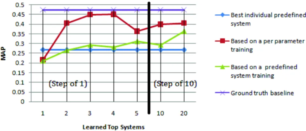
We also compare PPL method with two methods. The weak baseline is the system configuration (or predefined system) that has the best mean average precision (MAP) value over the test queries. This baseline is a weak one since it is not per query-based. The second baseline is the ground truth. It is the hardest baseline we can ever have. It is the average of AP over the test queries when using the best configuration for each query considered individually. Figure2shows a comparison between the PPL method (red square line) and the weak baseline in one hand and the ground truth on the other hand, represented by the blue and purple straight lines. We also compare the results with a fair baseline that corresponds to a method that that learns on a predefined systems basis (green triangles).
Figure2reports the MAP over the set of unseen test queries (averaged over the 10 draws resulting from 10-folds cross-validation) using the predicted configuration.
The PPL approach is efficient when predicting the best parameter values to be used for unseen queries. It is indeed very close to the hardest baseline; specifically when top 3 or 4 configurations per query are considered in the learning process. On the other hand, when learning predefined systems rather than learning parameter values, the predicted MAP is closer to the weak baseline whatever the number of top configurations per query used. Using such a simple approach will not add much improvement on the targeted problem.
Fig. 2. MAP - A comparison between the best predefined system, the PPL method, the predefined system classifier, and the ground truth method. The predictive functions are trained on top 1, 2 ,3, 4, 5, 10, and 20 systems per query (X-axis).
When considering only 4 top systems we can see that the PPL almost reach the ground truth, using more systems (up to 20 starts to lower the results. When learning on pre-defined systems, we need much more systems; it might be the case that adding more systems the green line can go upper, but using more systems is costly. Thus, for efficiency PPL is better. Using PPL method and considering 4 top systems, we go about 0.45 of MAP while learning on the predefined systems is about 0.27.
5. Conclusion
We present the PPL method that predicts the best configuration for an IR system for an input query, where such a predicted configuration optimizes a chosen effectiveness retrieval measurement. The PPL method learns each system parameter that controls an IR system individually. Since learning relies on query features, the best corresponding sys-tem configuration can be predicted for unseen queries. Intuitively, this methodology provides a more comprehensive and robust solution than relying on predefined system configurations in the training stage.
The experiments on TREC 7 & 8 topics from adhoc task show that the method is very reliable with good accuracy to predict a system configuration for unseen query. The results are close to the hardest baseline when considering more than one top system configurations per query in the learning process. Therefore, the PPL methods overcomes the problem of system variability.
In practice, using the number of configurations we used in the experiments reported in this paper could be prob-lematic. In future work, we will (i) analyze deeper the results in order to detect if some parameters have more impact on the final configuration that others. In that case, some parameters could be set to a predefined value while the other would be part of the learning; (ii) analyze the minimum number of predefined systems that are mandatory to generate the candidate training examples without decreasing the accuracy; (iii) study alternative means to calculate accuracy, less sensitive to a very small difference in effectiveness of the systems. We also use several other collections in order to measure the robustness of our method across collections.
References
1. G. Amati, C. Carpineto, and G. Romano. Query difficulty, robustness, and selective application of query expansion. Advances in Information
Retrieval, pages 127–137, 2004.
2. A. Bigot, C. Chrisment, T. Dkaki, G. Hubert, and J. Mothe. Fusing different information retrieval systems according to query-topics: a study based on correlation in information retrieval systems and trec topics. Information Retrieval, 14(6):617–648, dec 2011.
3. A. Bigot, S. Djean, and J. Mothe. Learning to Choose the Best System Configuration in Information Retrieval: the case of repeated queries.
Journal of Universal Computer Science, Information Retrieval and Recommendation, 21(13):1726–1745, 2015.
4. D. Carmel and E. Yom-Tov. Estimating the query difficulty for information retrieval. Morgan & Claypool Publishers, 2010.
5. R. Deveaud, J. Mothe, and J.-Y. Nie. Learning to rank system configurations. In Proceedings of the 25th ACM International on Conference
6. P. Goswami, M. R. Amini, and E. Gaussier. Transferring knowledge with source selection to learn ir functions on unlabeled collections. In Q. He, A. Iyengar, W. Nejdl, J. Pei, and R. Rastogi, editors, Conference on Information and Knowledge Management, CIKM, pages 2315–2320. ACM, 2013.
7. D. Harman and C. Buckley. The NRRC reliable information access (RIA) workshop. In Proceedings of the 27th annual international ACM
SIGIR conference on Research and development in information retrieval, pages 528–529. ACM, 2004.
8. P. Mohapatra, C. Jawahar, and M. P. Kumar. Efficient optimization for average precision svm. In Z. Ghahramani, M. Welling, C. Cortes, N. Lawrence, and K. Weinberger, editors, Advances in Neural Information Processing Systems 27, pages 2312–2320. Curran Associates, Inc., 2014.
9. J. Mothe and L. Tanguy. Linguistic features to predict query difficulty. In Predicting query difficulty - methods and applications Workshop,
Int. Conf. on Research and Development in Information Retrieval, SIGIR, pages 7–10, 2005.
10. J. Mothe and L. Tanguy. Linguistic analysis of users’ queries: towards an adaptive information retrieval system. In Signal-Image Technologies
and Internet-Based System, 2007. SITIS’07. Third International IEEE Conference on, pages 77–84. IEEE, 2007.
11. V. Plachouras, B. He, and I. Ounis. University of glasgow at trec 2004: Experiments in web, robust, and terabyte tracks with terrier. In Text
REtrieval Conference, TREC, 2004.
12. T. Qin, T.-Y. Liu, J. Xu, and H. Li. Letor: A benchmark collection for research on learning to rank for information retrieval. Information
Retrieval, 13(4):346–374, 2010.
13. A. Shtok, O. Kurland, and D. Carmel. Predicting Query Performance by Query-Drift Estimation. In Advances in Information Retrieval
Theory, Second Int. Conf. on the Theory of Information Retrieval, ICTIR, volume 5766 of LNCS, pages 305–312, 2009.
14. A. Shtok, O. Kurland, and D. Carmel. Predicting query performance by query-drift estimation. In Conference on the Theory of Information
Retrieval, pages 305–312. Springer, 2009.
15. S. Wu and S. McClean. Performance prediction of data fusion for information retrieval. Information Processing & Management, 42(4):899– 915, 2006.
16. Y. Yue, T. Finley, F. Radlinski, and T. Joachims. A support vector method for optimizing average precision. In Proceedings of the 30th annual
international ACM SIGIR conference on Research and development in information retrieval, pages 271–278. ACM, 2007.
17. Y. Zhou and W. B. Croft. Query performance prediction in web search environments. In Proceedings of the 30th annual international ACM