Genome-scale metabolic reconstruction and analysis of the Trypanosoma brucei metabolism from a Systems biology perspective

(1)

En vue de l'obtention du

DOCTORAT DE L'UNIVERSITÉ DE TOULOUSE

Délivré par :

Institut National Polytechnique de Toulouse (INP Toulouse) Discipline ou spécialité :

Pathologie, Toxicologie, Génétique et Nutrition

Présentée et soutenue par :

M. SANU SHAMEER

le mardi 26 avril 2016

Titre :

Unité de recherche : Ecole doctorale :

GENOME-SCALE METABOLIC RECONSTRUCTION AND ANALYSIS OF

THE TRYPANOSOMA BRUCEI METABOLISM FROM A SYSTEMS

BIOLOGY PERSPECTIVE

Sciences Ecologiques, Vétérinaires, Agronomiques et Bioingénieries (SEVAB) Toxicologie Alimentaire (ToxAlim)

Directeur(s) de Thèse : M. DANIEL ZALKO

Rapporteurs :

M. JEAN-PIERRE MAZAT, UNIVERSITE BORDEAUX 2 M. MATTHEW DEJONGH, HOPE COLLEGE

Membre(s) du jury :

1 M. JEAN-PIERRE MAZAT, UNIVERSITE BORDEAUX 2, Président

2 M. DANIEL ZALKO, INRA TOULOUSE, Membre

(2)

1

LIST OF ABBREVIATIONS

ACHR - Artificial Centering Hit and Run

ADP - Adenosine diphosphate

ALG11 - alpha-1,2-mannosyltransferase

ATP - Adenosine Triphosphate

BMC - BioMedCentral

BRENDA - BRaunschweig ENzyme DAtabase

BSF - Blood Stream Form

CDS - CoDing Sequence

ChEBI - Chemical Entities of Biological Interest

CMM - Creek Minimal Medium

CNS - Central Nervous System

COBRA - COnstraint-Based Reconstruction and Analysis

CTS - Chemical Translation Service

DHAP - DiHydroxy Acetone Phosphate

DNA - DeoxyriboNucleic Acid

EC - Enzyme Commission

EMBL - European Molecular Biology Laboratory

ER - Endoplasmic Reticulum

FBA - Flux Balance Analysis

FBS - Foetal Bovine Serum

FDA - Food and Drug Association

FVA - Flux Variability Analysis

GDLS - Genetic Design through Local Search

GIMME - Gene Inactivity Moderated by Metabolism and Expression GlcNAc2-PP-Dol - N-acetylglucosaminyl-diphosphodolichol

GlcNAc-PP-Dol - (N-acetylglucosaminyl)2-diphosphodolichol

GLPK - GNU Linear Programming Kit

GNU - GNU's Not Unix

GO - Gene Ontology

GPI - Glycophosphatidylinositol

GPL - General Public License

GPR - Gene Protein Reaction

HAT - Human African Trypanosomiasis

HTML - Hyper Text Mark-up Language

ID - Identifier

InChI - International Chemical Identifier

IUPAC - International Union of Pure and Applied Chemistry

JSON - JavaScript Object Notation

KEGG - Kyoto Encyclopedia of Genes and Genomes

KO - Knock-out

LP - Linear Programming

Man2GlcNAc2-PP-Dol - (mannosyl)2-(N-acetylglucosaminyl)2-diphosphodolichol

MIRIAM - Minimum Information Required In the Annotation of Models

(5)

4

NAR - Nucleic Acid Research

NCBI - National Centre for Biotechnology Information

NECT - Nifurtimox-Eflornithine Combination Therapy

NMR - Nuclear Magnetic Resonance

NP - Nondeterministic Polynomial time

PCR - Polymerase Chain Reaction

PDB - Protein Data Bank

PGDB - Pathway/Genome DataBase

RAST - Rapid Annotation using Subsystem Technology

RNAi - RiboNucleic Acid interference

SBGN - Systems Biology Graphical Notation

SBML - Systems Biology Mark-up Language

SEDML - Simulation Experiment Description Mark-up Language

SHTML - Server Side Includes (SSI) HTML

SILAC - Stable Isotope Labelling by Amino acids in Cell culture SMILES - Simplified Molecular-Input Line-Entry System

STITCH - Search Tool for Interactions of CHemicals

TbALG11 - T. brucei alpha-1,2-mannosyltransferase

TbALG2 - T. brucei alpha-1,3/1,6-mannosyltransferase

TbALG3 - T. brucei alpha-1,3-mannosyltransferase

UK - United Kingdom

URL - Universal Resource Locator

VSG - Variable Surface Glycoprotein

WHO - World Health Organization

(6)

5

LIST OF FIGURES

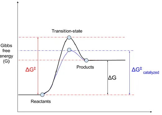
Figure 1 - The effects of enzyme catalysis in an endergonic reaction ... 12

Figure 2 – The central dogma of molecular biology ... 13

Figure 3 - T. brucei parasites in blood[225] ... 15

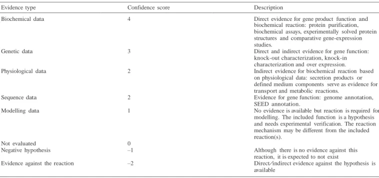
Figure 4 – Lifecycle of Trypanosoma brucei[30] ... 17

Figure 5 - A simplified representation of the Trypanosoma cell[42] ... 18

Figure 6 - Basic types of modelling in Systems Biology ... 22

Figure 7 - A simplified representation of the steps involved in genome-scale metabolic reconstruction, model validation and model prediction ... 29

Figure 8 – the phylogeny of constraint-based modelling approaches [114]... 34

Figure 9 - An illustration of sample metabolic model ... 35

Figure 10 – The solution space of the sample metabolic model ... 36

Figure 11 – Steps involved in using the simplex method in LP optimization ... 38

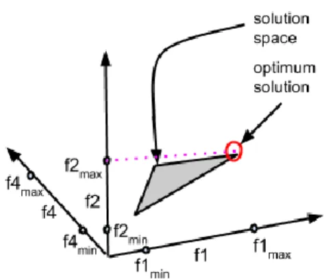
Figure 12 – The optimal solution of FBA analysis for the sample metabolic model ... 39

Figure 13– an example of for a phenotypic phase plane result ... 41

Figure 14– Scheme used to construct, update and synchronize the TrypanoCyc database and genome-scale metabolic network ... 57

Figure 15 – First three line of the TrypanoCyc update report... 70

Figure 16 – The online version of the TrypanoCyc update report ... 71

Figure 17 –LeishCyc on the TrypanoCyc website ... 72

Figure 18 – TrypanoCyc session statistics Nov 2013-15 ... 73

Figure 19 – TrypanoCyc usage statistics based on country ... 74

Figure 20 – TrypanoCyc usage statistics Nov ‘13 – Nov ‘15 ... 74

Figure 21 – Icon system used in TrypanoCyc to convey Pathway curation status ... 76

Figure 22 – Pipeline for the pre-processing of TrypanoCyc-based model ... 107

Figure 23– Trypanothione recycling in the metabolic model ... 109

Figure 24 – Protein N glycosylation in T. brucei ... 111

Figure 25 – edge width with respect to the flux observed through the reaction ... 113

Figure 26 – A thermodynamically infeasible loop in FBA solution ... 114

Figure 27 – Visualization of fluxes on the genome-scale metabolic model ... 116

Figure 28 – Contribution of essential nutrients in the iSS1077 model ... 120

Figure 29 – Optimizing iMAT results ... 122

Figure 30 – Search result for triosephosphate isomerise using new gene ID in popular databases .. 135

Figure 31– T.brucei arginase activity in KEGG and TrypanoCyc ... 136

Figure 32– Gene Ontology information on TriTrypDB ... 138

Figure 33 – Suggestion to include context specific constraints in sbml model ... 140

(7)

6

LIST OF TABLES

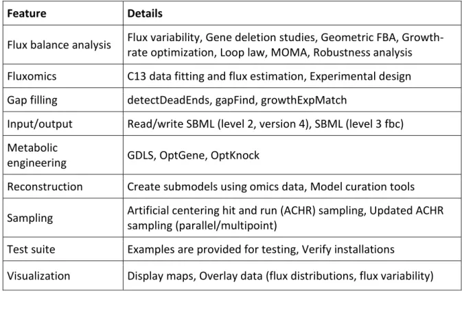
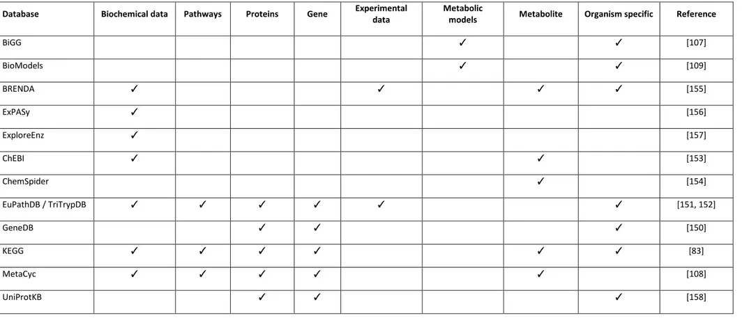
Table 1 - Features of COBRA Toolbox (version 2.0) ... 49 Table 2 - Summary of databases useful in model reconstruction ... 54 Table 3 – Popular tools used to analyze contain-based models ... 55 Table 4 –prediction accuracy of iMAT and optimized iMAT models built from Urbaniak et al [168] . 125 Table 5 Prediction accuracy of iMAT and optimized iMAT models built from Gunasekara et al [169] ... 126 Table 6 Comparison of prediction accuracy of iMAT and optimized iMAT models built from Vasquez et al [167] ... 127 Table 7 –Prediction accuracy of iMAT and optimized iMAT models built from TrypanoCyc comments ... 128

(8)

7

AKNOWLEDGEMENTS

First and foremost, I would like to show my sincere gratitude to my PhD supervisor, Dr. Fabien Jourdan for his encouragement, patience and continuous support throughout this project. His advices and suggestions have been vital to this thesis. I could not have asked for a better supervisor and mentor.

I would also like to show my gratitude to Prof. Jean-Pierre Mazat and Prof. Matt DeJongh for assigning a part of their most valuable time to review my work. I am positive that their insights and constructive comments on this thesis will help me in my future research. I would also like to thank Prof. Michael Barret (University of Glasgow) and Dr. Frédéric Bringaud (National centre for Scientific research – CNRS, Bordeaux) for taking the time from their busy schedule to monitor the progress of project. Besides being the assessors of the project, they have been extremely helpful throughout the project. Being a stranger to Trypanosoma metabolism at the beginning of the project, I owe them a great deal for the help they offered me in understanding this complex parasite. I would also like to thank Prof. David Westhead and Dr. Glenn McConkey from the University of Leeds for their advice and assessment with regards to the reconstruction and analysis of the metabolic model.

I would also like to acknowledge everyone from the MetExplore team members : Florence Vinson, Ludovic Cottret, Nathalie Poupin , Benjamin Merlet, Clément Frainay, Maxime Chazalviel and Florence Mourier; for their company and assistance throughout these 3 years. I have them to thank for the wonderful atmosphere we have at the lab.

I would also like to thank the TrypanoCyc annotation team. Without them, the TrypanoCyc database would have been but an empty shell. I would like to especially thank Prof. Fred Opperdoes, Prof. Peter Bütikofer and Fiona Achcar who went a step further by helping me understand the T.brucei metabolism.

I would also like to thank everyone from the ParMet group (www.paramet.eu). The program could not have been as smooth as it had been without the hard work put in by Prof. Sylke Muller, Amanda Baird and Karren Herron. Thanks to the ParaMet supervisors (PIs), experienced researchers (ERs) and early-stage researchers (ESRs); all consortium meetings were a perfect blend of scientific discussions, constructive feedbacks and fun activities.

I would also like to thank Suzette Domoulin and Marie-Helene Piquereau without whom procedures such as visa applications, university registrations and many, many other administrative tasks would have been Herculean for me. I would also like to thank everyone from Building A at INRA-Toxalim especially the members of MeX (Metabolism of Xenobiotics) team for the wonderful environment that I will definitely miss. I would also like to express my gratitude to Nicolas Cabaton, Vincent LeFol, Marie Tremblay-Franco and Roselyne Gautier for the company they gave me during the first few months at INRA when I was only beginning to meet people and make friends.

I would like to thank my parents for encouraging me to follow my own dream and for supporting me in all of my decisions academic and otherwise. Finally I would like to thank my wonderful wife who has been extremely patient and supportive of my research. I could not have finished this project without the support of my family and I owe all of my accomplishments, both small and large to them.

(9)

8

ABSTRACT

Recent advances in computational modelling of biological networks have helped researchers study the cellular metabolism of organisms. In this project, these approaches were used to analyze Trypanosoma brucei metabolism. This protozoan parasite is the causative agent of African trypanosomiasis, a lethal disease which has been responsible for huge loss of lives and livestock in Sub-Saharan Africa since ancient times. Information on T. brucei metabolism was gathered from published studies, databases and from personal communication with experts studying different areas of Trypanosomatid research. This information has been presented to the public through the TrypanoCyc Database, a community annotated T. brucei database. The database was published in November 2014 and has had over 4200 visitors from more than 100 countries as of November 2015. A manually curated genome-scale metabolic model for T. brucei was also built based on the gathered information to facilitate the study of T. brucei metabolism using systems biology approaches. Flux balance analysis based algorithms were designed to optimize visualization and study interesting metabolic properties. Blood-stream form specific metabolic models were generated using information available from published studies and the TrypanoCyc annotations with the help of the iMAT algorithm. Finally, an algorithm was designed to further optimize these stage specific models to improve the consistency of their predictions with results published in previous studies. These stage-specific models were observed to have a clear advantage over the genome-scale model when predicting stage-specific behaviour of T. brucei, particularly when predicting mutant behaviour.

(10)

9

(11)

10

1.1 METABOLISM

Metabolism is the set of physical and chemical processes that an organism is capable of performing in order to survive and reproduce [1]. The word ‘Metabolism’ was coined from the Greek term μεταβολή (metabolē - change) and ism (a suffix used to convert a verb as a noun) [2]

1.1.1 History of metabolism

Since the dawn of time man has been trying to understand the world around him. We made observations on the living and non living elements that interact with us and developed conclusions on why things happen the way they do. The rise of interest in agriculture and cattle breeding practices inevitably led to observations of the effect of food and other elements from the environment on cattle and crops. With the development of interest in the physiology of living beings, the effects of food and air on fellow humans and cattle were

observed by physicians such as Claudius Gaven. In the 1st century ,Gaven proposed that

pnuema, the fundamental principle of life according to Gaven, entered the body through air and from food into the blood [3]. However, the earliest recorded observations on

metabolism have been credited to Ibn al-Nafis who stated in 13th century in his theological

novel, ‘Al-Risalah al-Kamiliyyah fil Siera al-Nabawiyyah’ that "Both the body and its parts are in a continuous state of dissolution and nourishment, so they are inevitably undergoing

permanent change" [4]. Later in the 16th century, Sanctorio sanctorius performed studies on

himself and subjects by monitoring the weight of food, water, excrement and the human body before and after performing everyday activities and contributed to the study of an ‘insensible perspiration’ which tried to explain the disappearance of most of the food ingested [5].

Until Louis Pasteur’s revolutionary studies with fermentation in the 19th century, metabolic

processes were thought to be spontaneous. Pasteur observed that there was specific substances inside yeast, which he called “ferments”, that was responsible for fermentation [6][7]. However, it was believed that living matter possessed a vital force and was somehow different from non-living matter (the vitalist theory) [8]. In 1828, Friedrich Wöhler synthesized urea from ammonium cyanate and later in the century, Eduard Buchner was

(12)

11

capable of demonstrating the fermentation process using enzymes alone and without any live yeast [9]. This revelation opened up the field of biochemistry and fuelled the study of metabolic processes; and Buchner was awarded the Nobel prize in 1907 for his work [10]. With the development of powerful techniques in biochemistry, molecular biology and genetic engineering such as DNA sequencing (Fred Sanger), polymerase chain reaction or PCR (Kary Mullis), northern blotting (Alvin, Kemp and Stark), southern blotting (Edwin Southern), western blotting (Harry Towbin), X-ray crystallography (Max von Laue), mass spectrometry (J.J. Thompson), Nuclear magnetic resonance (NMR) spectrometry (Purcell and Bloch), electron microscopy (Ruska and Knoll), Gene knockout and RNA interference or RNAi

(Fire and Mello) by the 21st century, huge leaps in understanding metabolism were made.

1.1.2 Types of Metabolic processes

Through evolution, living beings have developed and optimized their metabolism to survive in their respective environments. Resources are procured from the surrounding by various means. These nutrients are then used directly or broken into smaller simpler compounds which are then used to build new larger biomolecules such as proteins, lipids, DNA, RNA, etc which are essential for growth and survival. Metabolism hence can be broadly classified into two major processes – anabolism and catabolism

a) Anabolism

Anabolism is the set of processes responsible for the synthesis of large biomolecules from their smaller precursors [1]. Starch and glycogen synthesis from glucose, lipid synthesis from acetyl-CoA, synthesis of proteins from amino acids, DNA and RNA synthesis from its

precursors are some examples of anabolism. The word anabolism was coined in the late 19th

century from the Greek word ἀναβολή (anabolē – throwing up) [11]. b) Catabolism

Catabolism on the other hand, refers to the biochemical breakdown of larger biomolecules into simpler compounds, which can later be used in anabolic processes or excreted into the environment. The release of energy associated with catabolism is very important for the growth and survival [1]. Protein degradation to amino acids, lipid breakdown into precursors

(13)

12

and glycolysis that generates energy (ATP) are some examples of catabolism. The word catabolism was derived from the Greek word καταβολή (katabolē – throwing down) [12]

1.1.3 Enzymes and regulation of Metabolism

Enzymes are large biomolecules responsible for catalyzing chemical reactions in cells. Most enzymes are proteins or protein complexes. The metabolic capabilities of a cell are directly related to the enzymes it is capable of expressing.

The first enzyme to be discovered was a diastase, the enzyme responsible for the breakdown of starch into maltose. It was discovered by the French chemists Payen and Persoz in 1833 [13]. Later in the same century, based on his observations, Louis Pasteur called the substance in yeast he believed to be responsible for fermentation as ‘ferments’[7]. Pasteur however proposed that the ferments would be active only in living cells and so it was not until 1877, that the word ‘enzyme’ was coined by Wilhelm Kühne to represent biomolecules responsible in catalyzing reactions even outside living cells [14].

Enzyme functioning is best explained by looking at the thermodynamics of their chemical

Figure 1 - The effects of enzyme catalysis in an endergonic reaction

The reaction for which the free energy (G) levels are illustrated in the figure was determined to an endergonic reaction owing to the a positive ΔG ( ΔG > 0 ). ΔG‡ is the activation energy required to initiate the reaction. Involvement of the enzyme reduces the free energy of the transition state and hence reduces ΔG‡ to ΔG‡catalyzed improving the chances of the reaction taking place.

(14)

13

reactions. The endergonic (energy consuming) or exergonic (energy producing) nature of chemical reactions is determined by the difference in the Gibbs free energy (ΔG) of its products and the substrates. The transition state theory proposed in 1935 suggests the formation of a transition state between the reactants and the products [15][16]. The transition state is believed to have a Gibbs free energy value higher than that of both the reactant and the product. This theory was capable of explaining why exergonic reactions also require a little energy to initiate the reaction. Hence in order to initiate a chemical reaction, an energy equivalent to difference in the Gibbs free energy of the transition state and the reactants (ΔG(transition-state – reactants) or ΔG‡) would be required. This energy is called activation

energy. Enzymes control the rate of chemical reactions by reducing the activation energy of chemical reactions. This happens with the help of the formation of an enzyme-substrate transition complex which requires a much lower activation energy [17]. Figure 1 represents the change in free energy of an endergonic reaction in the absence and presence of a catalyst.

As mentioned earlier, most enzymes are proteins or protein complexes. Proteins are encoded in the genetic material of organisms as genes. The enzyme-coding DNA or RNA gene is transcribed to messenger RNAs (mRNA) through a process called ‘transcription’ with the help of the enzyme RNA polymerase. A ribonucleoprotein complex called the ribosome then binds to mRNAs and synthesize polypeptide chains through the process called as ‘translation’. This transfer of information from the genes to proteins is the central dogma of molecular biology(Figure 2). The protein then may also go through post-translational modifications. Some of these proteins bind with other proteins to form catalytically active protein-complexes. Many proteins and protein complexes also require further modification

(15)

14

called ‘activation’ to form its catalytically active configurations.

Metabolism of a cell is regulated by direct regulation of enzymes activity or by regulating the availability of the enzyme by controlling the steps involved in protein formation. Regulation of its metabolism helps the cell to manage resources, deal with environmental stresses and allows them to specialize for performing specific functions (as in the case of multicellular organisms). Perturbation of enzyme activity has popularly been used by researchers to understand their function and relevance. Gene KO studies involve disrupting the genes coded in the genetic material making them unavailable for the transcription [18]. RNA interference (RNAi) technique is used to control gene expression at the post transcription level [19]. However unlike gene KO, RNAi only reduces the expression and does not eliminate it completely which makes them quite useful in studying essential genes [20–24]. Various approaches such as depleting available substrate levels, modifying protein structures, blocking active sites of enzymes, etc are also widely used by researchers to study enzyme activity [25, 26]. The metabolic changes between the perturbed and non-perturbed (wild type) cells help to understand the role of specific pathways or processes in the organism of interest [27, 28].

(16)

15

1.2 TRYPANOSOMA BRUCEI

Trypanosoma brucei is an insect-borne-protozoan parasite responsible for the potentially

lethal ‘African Trypanosomiasis’, also known as ‘sleeping sickness’ in humans and ‘Nagana’ in animals. The Tsetse fly (Glossina) is the vector responsible for the transmission of the T.

brucei parasite. African Trypanosomiasis has been reported exclusively in 36 countries of

sub-Saharan Africa which hosts the world’s entire Tsetse fly population [29]. The human T.

brucei strain has two major subspecies: T. brucei gambiense and T. brucei rhodesiense. They

are morphologically indistinguishable [30] but the gambiense strain is believed to account for 98% of the reported cases [29]. Figure 3 shows an image of T. brucei cells in blood.

1.2.1 History of T. brucei research

Pre-colonial times

The Trypanosoma family is supposed to have been around for a very long time and is believed to have been associated closely with the hominid evolution. This seems to be why humans are resistant to all species of Trypanosoma except the gambiense and rhodesiense as these subspecies are believed to have evolved later [31]. Veterinary papyrus of Kahun

Papyri believed to be from 2nd millennium BC ancient Egypt talks about a cattle disease

“ushau” during their time. The papyrus describes the symptoms of the disease which were similar to the symptoms of present day nagana [31, 32]. These ancient Egyptians are thought to have used an ointment from bird fat to prevent insects biting their cattle [31]. Abu Abdullah Yaqut, the famous Syrian slave turned geographer, talked about an underground village of dying inhabitants in the country of gold, a scene very similar to that of a sleeping

sickness epidemic. The oldest case report of sleeping sickness is from the 14th century by Ibn

Khaldoun who reported the death of Sultan Mari Jata of Mali with trypanosomiasis like

(17)

16

symptoms [31]. Arabian slave traders are also believed to have looked for swollen lymph nodes in the back of the neck to identify doomed slaves suffering from sleeping sickness before purchasing them according to the English physician, Thomas Winterbottom [33].

Colonial times

During the early days of the modern times, causalities on board slave ships led to an increased interest in the sleeping sickness. Doctors were pressed by ship captains and slave-traders to find the causative agent behind this strange disease [31]. British royal naval surgeon John Atkins in 1734 reported the symptoms of late(neurological) stage symptoms of sleeping sickness from his observations [33]. Later in 1803, Thomas Winterbottom published his report on sleeping sickness in which he reported the characteristic swollen lymph nodes in patients suffering from sleeping sickness [33]. One of the associations of nagana with tsetse flies was made by the famous Scottish medical missionary and explorer, David Livingston who lost his cattle to the disease in the Limpopo and Zambezi river valleys in 1852 [31][34]. In 1895, the Scottish pathologist and microbiologist David Bruce discovered trypanosomes in the blood of nagana affected cattle in Zululand for the first time [35]. In 1899, Plimmer and Bradford published a paper on the parasites naming it Trypanosoma

brucei after Bruce. In the same year, Frederick Walter Mott observed foreign mononuclear

cells in the brain of 2 Congolese patients during post mortem autopsies [36]. Soon later in 1901 Robert Michael Forde observed “wriggly worms” in the blood of a steam-boat captain from the river Gambia [37]. A few months later English physician Joseph Everett Dutton identified the parasites as trypanosome and named them T. gambiense in 1902 [31]. The link between trypanosomes and sleeping sickness was however not yet established [36]. In 1902, the Royal Society of London sent a sleeping sickness commission comprising of Cuthbert Christy (a British epidemiologist), George Carmichael Low (a Scottish clinician) and Aldo Castellani (an Italian bacteriologist) to the Uganda region [36]. Castellani then found trypanosomes in the cerebrospinal fluid of patients and identified them as the causative agent of Sleeping sickness for the first time [38]. Castellani thought these trypanosomes were different from T. gambiense based on the morphological features and named them T.

ugandensis [36], although they were found to be the same later. In 1903, Bruce reported

conclusive proof for the transmission of the parasites via tsetse fly [33, 36]. Bruce is reported to have thought the transmission was purely mechanical [31] and it wasn’t until 1909, when studies by the German surgeon Friedrich Karl Kleine showed that the transmission involved

(18)

17

life cycle stage transitions. Bruce then was later capable of describing the complete lifecycle of T. brucei [39]. The second subspecies of human trypanosomes, T.b.rhodesiense, was finally identified in 1910 by John William Watson Stephans & Harold Benjamin Fantham [39].

1.2.2 Lifecycle of T. brucei

The T. brucei parasite is capable of growing and multiplying in both the host (mammals) and the vector (tsetse fly) (See Figure 4). The insect stage begins as the parasite enters the tsetse midgut during blood meal from an infected person. Here the parasites transform into the procyclic trypomastigotes. These reproduce by longitudinal binary fission and move to the anterior part of the midgut where they transform into long mesocyclic trypomastigotes. The mesocyclic trypomastigotes then migrate to the salivary gland of the insect where they develop into epimastigotes attached to the salivary gland. These finally develop into the metacyclic trypomastigotes awaiting insect bite and transmission into a mammalian host. The metacyclic T. brucei parasites are transmitted through insect bite into the mammalian host.

In the blood these parasites develop into the long slender bloodstream forms which then reproduces through longitudinal binary fission. Symptoms of the hemolymphatic stage may include fever, swollen lymph nodes, severe headache and joint pain. The parasites are then

(19)

18

distributed through the circulatory system and reach the blood brain barrier. T. brucei is capable of crossing the blood brain barrier and infecting the brain and cerebrospinal fluid, leading to irreparable damage of the central nervous system (CNS). At this stage (the neurological phase), the host suffers from motion and speech disorder and erratic sleep pattern (giving the disease the name ‘sleeping sickness’). With the damage to the CNS, the host can fall into coma and eventually perish. Some slender trypomastigotes then irreversibly change to short stumpy forms in preparation for the insect stage [30]. African trypanosomiasis is lethal if left untreated, however cases have been reported where the hosts overcome the parasites but acts as a ‘healthy carrier’[40].

1.2.3 Characteristics of T. brucei cell

The T. brucei cell is typically 16-42µm [41] and has all the basic features of a eukaryotic cell. It is mononucleated, flagellated, has endoplasmic reticulum (ER), a single Golgi stack and an elongated mitochondrion [42]. The nuclear genome of T. brucei consists of 11 pairs of megabase chromosomes, intermediate and minichromosomes. Apart from this, being a member of the class Kinetoplastida, the parasite has a characteristic organelle in the mitochondrion called the kinetoplast that carries the mitochondrial DNA. Together with the nuclear genome, the total size of the T. brucei genome is 35 megabases per haploid genome [43]. T. brucei also have multiple peroxisome-like organelles that houses enzymes involved in important metabolic pathways such as glycolysis and isoprenoid biosynthesis called glycosomes [44]. Figure 5 represents a simplified representation of a Trypanosomatid cell.

(20)

19

Another interesting feature of the T. brucei cell is the presence of a Glycophosphatidylinositol (GPI) anchor linked protective coat. In the mammalian host, the protective coat is composed of variable surface glycoproteins (VSG) and protects the parasites from the host immune system [45]. In the insect stage, the protective coat is composed of GPI-anchored proteins called procyclins that protect the parasites from being digested by the insect’s enzymes [46].

1.2.4 Current Drugs and Treatment

The major task involved in trypanosomiasis treatment is early diagnosis. There have been four major drugs registered for trypanosomiasis. Pentamidine and suramin are used to treat early stage (hemolymphatic stage) of T.b.gambiense and T.b.rhodesiense infections respectively. Melarsopol and eflornithine are the drugs used to treat the second (neurological) stage of Human African Trypanosomiasis (HAT) with eflornithine being effective only against T.b.gambiense [29]. Although these are life saving drugs provided free of cost to the affected countries [47], they cause adverse side effects in patients with some of them even being fatal. Particularly in the second stage treatment, the drug action involves crossing the blood-brain barrier and killing the parasite which can sometimes lead to reactive encephalopathy. This lack of an efficient treatment regime is the key driving factor in African trypanosomiasis research. Recently Nifurtimox-Eflornithine combination therapy (NECT) has been found to more successful in patients in the neurological phase of the infection [48][49] and is now the recommended therapy by World Health Organization (WHO). However even this treatment report multiple adverse side-effects. In the 1735 patients from 9 countries under NECT treatment, monitored in 2010-11, at least one adverse event was reported in 60.1% of the patients and a total of 3060 adverse events were reported. 9 deaths were also reported in the study with cause of death owing to reactive encephalopathy [48]. There is hence still a need for a more efficient treatment regime against African Trypanosomiasis.

Eflornithine is the only anti-Trypanosomiasis drug approved for use for which the mode of action has been conclusively determined. It depletes the amount of catalytically active ornithine decarboxylase in T. brucei cells which hampers Trypanothione biosynthesis and makes the cell susceptible to oxidative stress [50]. It is also the most efficient of

(21)

anti-20

Trypanosomiasis drugs. There is hence a clear advantage in using drugs targeting specific metabolic processes. And so the study the parasite metabolism to identify essential metabolic processes and the use of target based drug screening/designing approaches could lead to the discovery of other more efficient drugs against Trypanosomiasis.

(22)

21

1.3 SYSTEMS BIOLOGY

1.3.1 Introduction to systems biology

Traditional research in biology drew its roots from physics and chemistry. And hence it also inherited the reductionist mechanistic approach of study which was made popular by René Descartes, Isaac Newton and other great minds of their time. Based on this approach, all components of a cell could be studied individually and the behaviour of the cell can be predicted by combining the results of the individual studies. An example of the successful interpretation of this theory for higher plants was made by Jacques Loeb from his observations on the responses of seedlings to light and gravity which was published in 1912. Aristotle, the Greek physician is believed to have stated that “the whole is something over and above its parts and not just the sum of them all” [51]. With the popularity of the

reductionist mechanistic approach in physics in the 17th century, Aristotlean views were

shelved [52]. It wasn’t until Paul Weiss’s study on the effects of light and gravity on insect behaviour that conclusive experimental proof against the mechanistic theory was found [53]. He observed that although the final phenotypic response to the stimuli was identical among individuals, the series of responses that led to the final phenotype was different among them. This brought back the ‘whole is greater than the sum of the parts’ concept proposed by Aristotle. The renewed interest also led to the coining of the term ‘holism’ by Jan Smuts [54] and the popularity of Systems Biology, the holistic approach of studying complex biological systems.

Kirschner in 2005 stated that the formulation of a definition for Systems Biology is a difficult task. As a start, he suggested that Systems Biology is the study of the behaviour of complex biological organization and processes in terms of the molecular constituents [55]. The organism level study of biological systems involves the integration of multiple wet-lab (cell biology, biochemistry, etc) and dry-lab (mathematical modelling, bioinformatics, etc) approaches. With the development of the next-generation sequencing and ‘omics’

technologies in the 21st century, a massive amount of genomic, proteomic and metabolic

information was made available to researchers. The effective combination of this mountain of information essentially requires a mathematical model in the form of a network of

(23)

22

metabolites, proteins and the genes-catalyzing-them. The type of modelling used depends on the type of the data available and the aim of the study. For example, metabolic models help study cellular metabolism and regulatory networks help study regulation in cells. Large networks such as genome-scale networks are impossible to analyze by hand. However, with the advancement in computational approaches in mathematical modelling, it is now possible to study and understand these biological networks.

1.3.2 Types of Modelling in Systems Biology

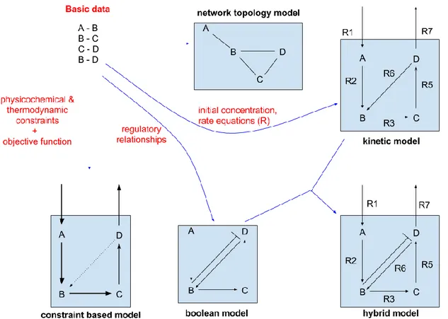
Since the rise of Systems Biology, multiple mathematical approaches have been developed to study life (Figure 6). Based on the data modelled, available biological information, the complexity of the data and the objective of the study; modelling approaches can be classified as following:

a) Network topology studies

Network topology approach in studying biological systems is the most basic of modelling

(24)

23

studies in systems biology. This approach is most useful in the case of extremely large network lacking detailed information. The model is studied as a network of nodes representing metabolites or reactions or both connected by edges. The edges of a network can be directed or undirected depending on the type of biological data. Protein-protein interaction networks usually have undirected edges while metabolic networks have directed edges. Analyses such as network robustness, centrality studies, modularity studies, network motif analysis, identification of network hubs, etc help gain important insights into the organization of system elements such as identifying vulnerabilities, important pathways and regulators [56]. The network topology approach however does not take into consideration the time and physiological context of the biological systems [57]. Network topology approach has been applied in the study of transcription factor binding networks [58], protein-protein interaction networks [59], protein-phosphorylation networks [60], metabolic interaction networks [61][62], genetic and small molecule interaction networks [63] and co-expression networks [64].

b) Boolean modelling

A Boolean network is a set of nodes capable of only binary values (1 or 0, ON or OFF) related by logical functions. These functions involve a combination of AND, OR and NOT operations on the values of other nodes [65]. The set of the Boolean values of nodes in the model is considered as the state of the model [66]. Boolean networks add a dynamic level to the basic network. The set of logical functions determining the transition of the model can be used to

predict the next state of the model. A Boolean network of n nodes has a solution space of 2n

network states [66]. Boolean modelling simulations can lead to prediction of steady states in the solution space (also known as attractors) and the set of initial states capable of achieving the steady states (also known as the basin of attraction) [66]. Boolean modelling approach has proven very useful in the study of regulatory [67] and signalling networks [68].

c) Constraint-based modelling

The constrained-based modelling approach in systems biology involves defining a model as a set of linear equations with constraints to restrict the solution space. In the case of metabolic networks, the reactions are converted to linear equations with the metabolites as coefficients and reactions becoming variables. Constraints on the reactions are set based on

(25)

24

the law of conservation of mass, reactions thermodynamics and available experimental data [69]. Unlike kinetic modelling, the constrain-based approach does not require information from enzyme kinetics studies or initial metabolite concentrations, making them the go-to choice for large metabolic networks such as genome-scale metabolic models [61, 70–73]. The flow of metabolites in the model is represented by a “flux” through the reactions. This metabolic flux is represented as number of metabolites per gram dry weight per unit time (mmol/gDW/hr). Multiple algorithms have been developed to study constraint-based models, the most popular being the flux balance analysis [74].

d) Kinetic modelling

Kinetic modelling involves representing the biological system as a set ordinary differential equations (ODEs) or partial differential equations (PDEs) and solving them in order to predict the state of the system after a given period of time [75, 76]. Kinetic modelling uses additional information on the system elements such as metabolite concentrations, reaction rates and compartment size to perform dynamic simulations. Determining reaction rates require detailed reaction kinetics studies of the reactions involved in the model [77]. Reaction rate equations use information from reaction kinetics to calculate the change in concentration of the metabolites as a function of time. Kinetic models can be simulated using either deterministic or stochastic algorithms. Limitation to kinetic modelling include the difficulty in determining the kinetics of reaction involved and computationally expensive algorithms especially in the case of stochastic simulations greatly limiting the size of the model [75].

e) Hybrid modelling approach

All approaches in modelling of biological systems have their own positive and negative aspects. Furthermore, different approaches are used to study the different levels of cellular mechanism such as Boolean modelling for regulatory networks and kinetic modelling for metabolic networks. Studying these processes separately leads to the loss of certain influence on their results [78]. Owing to these reasons, recently there have been efforts to combine the various approaches in order to reduce limitations and improve application. Hybrid modelling has been used to study the E. coli central metabolism [79], mucus production in Pseudomonas aeruginosa [80], integrating signalling with transcription

(26)

25

regulation and metabolism [81], etc. With the development of efficient algorithms, improving reliability of results and overall ability to model different levels of the cellular machinery, the hybrid modelling approach seems to be the future direction of computational systems biology.

As mentioned earlier, the choice of modelling approach used in a study depends on the objective of the study and the data available. This research project aims is to analyze the cellular metabolism of T. brucei. And so given that the annotated genome of T. brucei was published in 2008 [82] and biochemical databases such as KEGG [83] has been successful in gathering information and making it available to the scientific community, the constraint-based modelling approach was selected for use in this project. And so detailed description of this technique and the algorithms used to study these models are discussed in the next chapter.

(27)

26

1.4 CONSTRAINT-BASED MODELLING AND GENOME-SCALE

METABOLIC RECONSTRUCTION

Note to the reader

This section shares much of its content with the chapter, “Understanding Protozoan

Parasite Metabolism and Identifying Drug Targets through Constraint-based Modelling”

authored by Francis Isidore Totanes, Sanu Shameer, David R. Westhead, Fabien Jourdan and Glenn A. McConkey (see APPENDIX 1 for the abstract and complete text). The chapter was accepted as part of the book titled “Analysis of parasite biology – from metabolism to drug

discovery”. The book is edited by S. Müller, R. Cerdan and O. Radulescu and will be volume 7

of the Wiley Book Series, Drug Discovery in Infectious Diseases.

1.4.1 Genome-scale metabolic models

A genome-scale metabolic reconstruction or model is a representation of a cell as a network of all the metabolic reactions that have been identified to occur within the given cell. Organism-level systems biology involves the use of large datasets from high-throughput measurements, reconstruction of cellular systems, mathematical modelling and in silico simulations [84]. The main objective of this approach is to provide an understanding of the workings of complex biological systems and to attain this development of mathematical models is required. These models attempt to closely replicate wet lab experiments with the goal of computationally generating hypotheses at the organism level (also called genome scale) that can be experimentally validated [85]. Genome sequencing data, knowledge on gene-protein-reaction (GPR) relationships, and biochemical and enzymatic data on the metabolism of an organism are combined to create a genome-scale model. Computation based on these models allows the calculation of possible phenotypic states of the model organism [74]. Genome-scale models can also be used to predict the function of previously uncharacterised genes and rectify incorrectly annotated genes. Gene deletions, gene over- or under-expression strategies are applied to genome-scale models to predict genes and pathways that may be altered for bioengineering the production of therapeutically- or industrially-important compounds [86]. These models can also be used to predict genes and

(28)

27

enzymes that are essential for the survival of an organism. These predicted essential genes and enzymes may be potential drug targets and therefore important in drug discovery and development [87].

Genome sequence and gene annotation data are used to identify specific roles of individual proteins within the system. A metabolic network (i.e. a network of metabolites interconnected via reactions involving the said metabolites) is developed utilising published data on elucidated protein function and cellular location, enzyme thermodynamics and reaction stoichiometry. Data from closely related organisms, e.g. orthologous gene data, are sometimes used in the absence of reported information on the organism of interest [88]. Reactions and corresponding metabolites are tabulated into a matrix that accounts for the number of metabolites consumed and produced within the given reactions. Additional constraints on the fluxes through the reactions (often expressed in metabolite amount per dry weight of the parasite per hour) with upper and lower boundaries are incorporated to control the flux values and represent the reversibility of reactions [89].

1.4.2 Constraint-based Modelling

Constraint-based modelling is an important in silico approach which takes into account the different biochemical processes (i.e. reactions) and the flow of metabolites (i.e. species) in order to closely represent the metabolic network of an organism without the necessity for individual enzyme kinetics. It models the possible steady-states of the metabolic network (a state at which the metabolite concentrations do not change over time) because of which

enzyme kinetic parameters (e.g. Michaelis constant KM) that would need to be derived from

recombinant expression and biochemical assays for all enzymes are not required. This is an important advantage for genome-scale modelling since these parameters are seldom known for every enzyme encoded in a genome. Moreover, these enzyme parameters are strongly dependent on environmental conditions (pH for instance). Even with the steady state assumption, too many fluxes will need to be computationally predicted. In order to focus on more relevant flux distributions, specific constraints, often based on experimental data, are entered into the system to represent limits of enzymatic fluxes as well as available metabolites. The steady state assumption allows the use of linear programming (i.e. a mathematical technique that computes the optimal output of a model whose constraints are

(29)

28

given by a set of linear equations) to solve for the maximum or minimum flux values [74] . Finally, the growth of the organism is predicted based on the production of essential components required for biomass production [90].

Constraint-based modelling has been used to predict the cellular response of an organism in different conditions. This allows a more in-depth comprehension of the complex metabolic networks in organisms [91]. As a result, functional annotations for hypothetical proteins and correction of erroneous annotations are possible [89]. By restricting the amount of specific metabolites, changes in the production of biomass components in constraint-based models can be used to predict the growth rate of the organism [92]. Single gene knockout simulations in constraint-based modelling have been used to pinpoint possible drug targets against pathogenic organisms [89]. Constraint-based modelling of cellular networks have been utilised in order to identify drug targets in cancer cells [93]. This technique can also be utilised in the development of bacterial strains used for the production of metabolites of nutritional or pharmaceutical interests. Gene knockouts that will redirect the consumption of precursor metabolites to allow the overproduction of metabolites of interest can be identified using flux balance analysis [94].

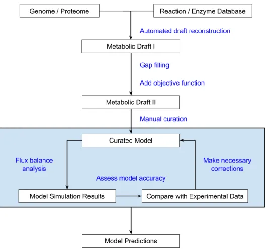
1.4.3 Steps in genome-scale metabolic reconstruction

Genome-scale metabolic reconstruction involves two stages – an automated reconstruction and a manual curation stage. Figure 7 describes a simplified protocol for genome-scale reconstruction

a) Automated Genome-scale Metabolic Network Reconstruction

As mentioned earlier, a genome-scale metabolic reconstruction is a representation of a cell as a network of all the metabolic reactions that have been identified to occur within the given cell. As it is time consuming to manually add every single reaction one after the other, many automated tools [95–97] and algorithms have been developed to help generate a draft which can then be manually curated to better describe the cellular network.

Automated genome-scale draft reconstruction tools use an annotated genome of the organism of interest to mine biochemical databases (or reactions pools) in order to identify a set of reactions associated with the enzymes encoded in the genome. Some of these tools

(30)

29

also predict the cellular localization of the enzymes in order to develop multicompartment models. This subset of chemical reactions along with their gene-protein-reaction relationship forms the draft of the metabolic reconstruction [98]. Some automated genome-scale metabolic reconstruction tools such as the SEED server is even capable of annotating the genome of interest and have proved to be quite efficient with prokaryotic reconstructions [99]. All automated draft reconstruction tools have their own reaction pools from which reactions are selected for the draft. PathoLogic, the automated draft reconstruction tool employed in Pathway Tools, for instance uses the MetaCyc database as its pool [96]. The AUTOGRAPH pipeline is well known for implementing the use of a user-defined manually curated metabolic model as the reaction pool for generating the initial draft [97]. More details on these tools will be discussed further later on in this write-up.

Most draft reconstruction tools and servers use non-organism specific reaction pools to enable their application on diverse species. These drafts are hence prone to false positive

Figure 7 - A simplified representation of the steps involved in genome-scale metabolic reconstruction, model validation and model prediction

(31)

30

and false negative hits that results in the draft containing reactions known to be absent in the organism of interest and not containing reactions which are known to be present in the organism of interest respectively. Organism specific reactions which are absent in the reaction pool are also missed in these automated reconstructions. Many automated genome-scale reconstructions also fail to identify and incorporate transport reactions into the model. Manual curation is hence necessary to fix these issues and create a more realistic representation of the genome-scale metabolism of interest [100].

b) Manual Refinement of Genome-scale Model

The manual curation step in genome-scale reconstruction involves modifying the model draft so that it better represents the organism in real life. It involves adding reactions missing in the draft and removing reactions known not to exist in the organism of interest. The manual curation stage involves re-evaluation and refinement based on literature and experimental observations. The manual curation stage is in essence a never ending process. It is usually coupled with simulation and validation of the model with experimental data in order to identify how well the model is able to represent the actual metabolism. Another important part of manual curation is the addition of metadata to the model such as InChI and SMILES identifiers to the metabolites, and Enzyme Commission (EC) number, pathway and enzyme localization information to the reactions. With the recent increase in genome-scale metabolic reconstructions, detailed protocols for manual curation have been published [100].

c) Standardization and Model Formats

In 2005, Le Novère et al. reported that "most of the published quantitative models in biology are lost for the community because they are either not made available or they are insufficiently characterized to allow them to be reused” [101]. With the increasing importance of metabolic models in research, standard formats were established to improve exchange and reusability. Currently metabolic models are accepted in the scientific community in the form of standardized machine readable formats such as Systems Biology Markup Language (SBML) [102], CellML [103], BioPax [104], etc. Additionally specific standards were developed to encode graphics notations (SBGN) [105] and simulation descriptions (SedML) [106].

(32)

31

One of the major issues that affect the understanding and reusability of existing metabolic models is the lack of a single identifier system for metabolites and reactions. This leads modellers to generate their own identifiers or borrow identifiers from popular biochemical databases such as Kyoto Encyclopedia of Genes and Genomes (KEGG) [83], Biochemical Genetic and Genomic (BiGG) [107] and BioCyc [108]. Since genome-scale reconstructions tend to have thousands of reactions and metabolites, the use of different ID systems makes the comparison of models or mapping experimental data difficult and time consuming. As a result, the scientific community stresses on the inclusion of metadata along with the model elements in the form of annotations. Some modellers also provide additional information on model components in the form of InChI, SMILES, EC numbers, etc. The Minimum Information Required In the Annotation of Models (MIRIAM) guidelines published in 2005 [101] describe an efficient solution to this problem. According to the MIRIAM guidelines the model should clearly provide a description of all model elements, relate to a publication, list its authors and contact information along with the simulation conditions. In the case of model elements annotations, the MIRIAM guidelines advice authors to link those to external databases using an annotation triplet: "data-type", "identifier" and "qualifier". Here the "data-type" refers to the general part of the link to a database resource and the "identifier" refers to the specific ID in the particular database. The "qualifier" is a term (selected from a predefined namespace) used to represent the relationship to the resource. According to the BioModels database [109] there are two types of qualifiers, a) model qualifier that represents the relationship between a modelling object and its annotation and b) biological qualifier that represents the relationship between a biological object represented by a model element and its annotation [110]. The implementation of the MIRIAM guidelines can thus improve the reusability of metabolic models. However, since different modellers can use references to different database resources, comparison of different models implementing different identifier systems is still not straightforward. The InChI system [111] developed by International Union of Pure and Applied Chemistry (IUPAC) provides a unique identifier for a chemical entity (i.e. metabolite) and hence this can be used to determine identical metabolites and reactions between two different models. With the implementation of these standardizations, metabolic models developed can be easily read, understood, integrated with experimental data and even combined to generate larger metabolic models.

(33)

32

1.4.4 Examples of genome-scale reconstruction in other

Trypanosomatids

a) Leishmania major

Chavali et al. [89] developed a reconstruction of the Leishmania major metabolic network utilising published literature and gene/enzyme databases. The network takes into account a total of 560 genes, 1,112 reactions and 1,101 metabolites. Stoichiometric equations of metabolic reactions were atom- and charge-balanced, and thermodynamic properties of these equations were also considered. Biomass production was assigned as the overall objective of the metabolic network. Biomass components include amino acids, fatty acids and DNA. The estimated amount of amino acid per gram of dry weight was computed based on the open reading frames in the genome of the organism, while the DNA component was computed by taking into account the G-C content of L. major DNA. Fatty acid components were based on previously published literature. For the computation of fluxes, subcellular locations of the different reactions were also considered. Linear programming optimization was used to compute the flux distribution for the entire network at maximum biomass production.

To identify essential genes, single and double gene deletions were simulated by forcing zero flux through reaction/s associated with particular gene/s. The effect of the deletion on the growth of the organism was then categorised as lethal (0% growth), growth-reducing (between 0 and 90% growth) and no effect (greater than 90% growth). Lethal double gene deletions were further classified as either trivial or non-trivial. A total of 69 lethal single gene deletions were identified, while 19,285 and 56 trivial and non-trivial double gene deletions were identified, respectively [89]. Furthermore, using the sequences of the enzymes involved in the predicted set of essential reactions, inhibitors (e.g. antipsychotics and antibiotics) were identified from existing drug databases and were tested experimentally for target validation [112].

b) Trypanosoma cruzi

The iSR215 is a metabolic network reconstruction of Trypanosoma cruzi strain CL Brenner core metabolism developed by Roberts et al. [113]. In this study, two models were

(34)

33

created for T. cruzi. The full model was based on direct genetic and biochemical data involving T. cruzi as well as data on other related species obtained from published literature. It takes into account 215 genes and 162 reactions in four subcellular compartments. Another model simulated the metabolic network of the epimastigote form of the parasite. Proteomic data from epimastigote cultures was obtained to identify specific proteins that are present in this stage of the parasite. Proteins absent in the epimastigote are removed from the full model by forcing a null flux into the involved reactions. Redirections of metabolic fluxes through certain pathways in the epimastigote model was observed as a result of the absence of trypomastigote and amastigote stage-specific reactions. The model was validated by comparing the predicted metabolic by-products in aerobic and anaerobic conditions with data presented in published literature. By-products observed in the model were found to be mostly consistent with data reported in literature.

Single reaction knockouts were predicted for each reaction in the full and the epimastigote models. A greater number of lethal reaction knockouts (40 reactions) were observed in the epimastigote model compared with that of the full model (26 reactions). This has been associated with the limitations imposed by the redirection of pathways in the absence of a number of reactions in the epimastigote model. Double reaction knockouts were also simulated in both models. Similarly, the epimastigote model yielded greater number of trivial and non-trivial deletions, 2,880 and 183, respectively, as compared with the full model (1,872 and 96, respectively). The predicted essential reactions were then compared with published experimental data species related to T. cruzi to further validate the results of the metabolic model. Forty-six out of the 58 published gene targets available were consistent with the results of the metabolic network. All non-lethal reactions in published literature were consistent with the results of the network [113].

1.4.5 Methods to analyze constraint based models

With the recent rise in popularity of constraint-based models, a huge number of approaches and algorithms have been developed to answer various biological question using constraint based models. Lewis et al managed to cluster the different approaches into approaches for integrating ‘omics’ data, integrating regulatory mechanisms, thermodynamic parameter based optimization, loop removal, objective function development, gap-filling, reaction

(35)

34

perturbation design, reaction addition design, gene-deletion design, flux balance analysis (FBA) based approaches and objective function independent analyses [114]. Figure 8 displays a more detailed view of this classification. FBA-based approaches are the most popularly used approaches to study metabolism. Here we will discuss the FBA algorithm and some of it widely used extensions.

a) Flux balance analysis of genome-scale metabolic models

Flux balance analysis is a mathematical approach to study the flow of metabolites in a constraint-based model when assuming the model to be at steady state (i.e. the concentration of metabolites in the model is constant). The first step to flux balance analysis is the creation of a mathematical representation of the metabolic reactions in a given metabolic network. Reactions and corresponding metabolites involved in specific reactions are tabulated into a matrix (i.e. Stoichiometric matrix, or S-matrix) that accounts for the number of metabolites consumed and produced within the given reactions. Columns of the

(36)

35

matrix represent the reactions while rows represent the metabolites. The number of metabolites produced or consumed in a given reaction is represented in the matrix as a positive or negative number, respectively. The stoichiometry of metabolites in each reaction provides a constraint onto the resulting network.

Consider a network of m metabolites and n reactions for which the S-matrix, a sparse matrix

of size ‘m × n’ is S. If v is a vector of fluxes f1,f2,…,fn for the n reaction i.e. then when

assuming steady state S.v = 0

In addition to the stoichiometry based constraints, each reaction is assigned a flux boundary (i.e., upper and lower bounds) which represent the permissible fluxes for the said reaction. These constraints therefore define the allowable rates at which metabolites are produced or consumed within the system [74].

If fi is the flux through reaction i in the network, then fiMIN ≤ fi ≤ fiMAX where fiMIN and fiMAX

is the lower and upper bounds of flux through the reaction i respectively.

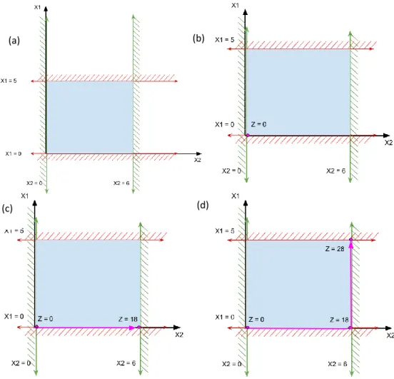
Following the creation of the S-matrix and the assignment of flux boundaries for the reactions, an objective function is selected based on the study. A reaction representing the said function (e.g., production of biomass components from precursors [90]) is included into the matrix. Biomass reactions, for example, are either based on experimentally obtained data [71][74] or from data obtained from closely related organisms [89, 115].

Consider the metabolic model described in Figure 9 comprising of metabolites A-F and

Figure 9 - An illustration of sample metabolic model

A, B, C, D and E are metabolites of the sample metabolic network. R1, R3 and R4 are reactions in the sample metabolic network. B is the metabolite contributing to the biomass of the sample model through the reaction R2. f1, f2, f3 and f4 are the fluxes through R1, R2, R3 and R4 respectively

(37)

36

reactions R1-R4 carrying a flux of f1-f4. Such that R1: A  B + C

R2: 2B  R3: C  D R4: B  E

And R2, the consumption of 2 molecules of B, is considered as the objective function of the model.

If A,D and E are boundary metabolites (i.e their concentration in the environment is so large compared to the other metabolites in the system that very negligible change in

concentration is observed), they are excluded from the S- matrix

Then the S-matrix for the model, ; f and

the objective coefficient vector, C =

Since the model is assumed to be at steady state, S.v = 0

i.e.

Using these stoichiometric constraints, we have the following system of linear equations representing the model

f1 –f2-f4 = 0, f1-f3=0

=> f2 = f1 - f4, f1 = f3

Next based on the flux constraints we have

Figure 10 – The solution space of the sample metabolic model