To link to this article : DOI :
10.1016/j.neuroimage.2016.08.064
URL :
https://doi.org/10.1016/j.neuroimage.2016.08.064
To cite this version :
Costa, Facundo and Batatia, Hadj and Oberlin,
Thomas and D'Giano, Carlos and Tourneret, Jean-Yves Bayesian
EEG source localization using a structured sparsity prior. (2017)
NeuroImage, vol. 144 (Part A). pp. 142-152. ISSN 1053-8119
O
pen
A
rchive
T
OULOUSE
A
rchive
O
uverte (
OATAO
)
OATAO is an open access repository that collects the work of Toulouse researchers and
makes it freely available over the web where possible.
This is an author-deposited version published in :
http://oatao.univ-toulouse.fr/
Eprints ID : 18798
Any correspondence concerning this service should be sent to the repository
administrator:
[email protected]
Bayesian EEG source localization using a structured sparsity prior
Facundo Costa
n,a, Hadj Batatia
a, Thomas Oberlin
a, Carlos D'Giano
b, Jean-Yves Tourneret
aaUniversity of Toulouse, INP/ENSEEIHT - IRIT, 2 rue Charles Camichel, BP 7122, 31071 Toulouse Cedex 7, France bFLENI Hospital, Buenos Aires, Argentina
Keywords: EEG MCMC Inverse problem Source localization Structured-sparsity Hierarchical Bayesian model ℓ20norm regularization Medical imaging
a b s t r a c t
This paper deals with EEG source localization. The aim is to perform spatially coherent focal localization and recover temporal EEG waveforms, which can be useful in certain clinical applications. A new hier-archical Bayesian model is proposed with a multivariate Bernoulli Laplacian structured sparsity prior for brain activity. This distribution approximates a mixed ℓ20pseudo norm regularization in a Bayesian
framework. A partially collapsed Gibbs sampler is proposed to draw samples asymptotically distributed according to the posterior of the proposed Bayesian model. The generated samples are used to estimate the brain activity and the model hyperparameters jointly in an unsupervised framework. Two different kinds of Metropolis–Hastings moves are introduced to accelerate the convergence of the Gibbs sampler. The first move is based on multiple dipole shifts within each MCMC chain, whereas the second exploits proposals associated with different MCMC chains. Experiments with focal synthetic data shows that the proposed algorithm is more robust and has a higher recovery rate than the weighted ℓ21mixed norm
regularization. Using real data, the proposed algorithm finds sources that are spatially coherent with state of the art methods, namely a multiple sparse prior approach and the Champagne algorithm. In addition, the method estimates waveforms showing peaks at meaningful timestamps. This information can be valuable for activity spread characterization.
1. Introduction
EEG source localization problem has attracted considerable attention in the literature resulting in a wide range of methods developed in the last years. These can be classified into two groups: (i) the dipole-fitting models that represent the brain ac-tivity as a small number of dipoles with unknown positions; and (ii) the distributed-source models that represent the brain activity as a large number of dipoles in fixed positions. Dipole-fitting models (Sommariva and Sorrentino, 2014;da Silva and Van Rot-terdam, 1998) try to estimate the amplitudes, orientations and positions of a few dipoles that explain the measured data. Un-fortunately, the corresponding estimators are very sensitive to the initial guess of the number of dipoles and their initial locations (Grech et al., 2008). On the other hand, the distributed-source methods model the brain activity using a large number of dipoles with fixed positions and try to estimate their amplitudes (Grech et al., 2008) by solving an ill-posed inverse problem. One of the most simple ways to solve this inverse problem is to use an ℓ2
norm regularization as the minimum norm estimator (
Pascual-Marqui, 1999) or its variants Loreta (Pascual-Marqui et al., 1994) and sLoreta (Pascual-Marqui et al., 2002). However, these methods usually overestimate the active area size (Grech et al., 2008).
Sparsity constraints can remedy the overestimation issue when dealing with applications with discretely localized activity such as certain kinds of epilepsy (Berg et al., 2010). In distributed activity ap-plications, promoting sparsity should provide spatially coherent loca-lization even though it is unable to estimate the activity extension. To apply sparsity, ideally an ℓ0 pseudo norm regularization (Candes, 2008) should be used. Unfortunately, this procedure is intractable in an optimization framework. As a consequence, the ℓ0pseudo norm is
usually approximated by the ℓ1norm via convex relaxation (Uutela et al., 1999), even if the two regularizations do not always provide the same solution (Candes, 2008). In a previously reported work, we proposed to combine them in a Bayesian framework (Costa et al., 2015), using the ℓ0pseudo norm to locate the non-zero positions and
the ℓ1 norm to estimate their amplitudes. However the methods
studied inCandes (2008),Uutela et al. (1999), andCosta et al. (2015)
consider each time sample independently leading in some cases to unrealistic solutions (Gramfort et al., 2012).
To improve source localization, it is possible to make use of the temporal structure of the data. This can be done by considering sparse Bayesian learning using multiple measurement vectors (Zhang and Rao, 2011) or by using the STOUT (Castaño-Candamil et al., 2015) and dMAP-EM (Lamus et al., 2012) methods that apply
n
Corresponding author at: INP - ENSEEIHT Toulouse 2, rue Charles Camichel, B.P. 7122, 31071 Toulouse Cedex 7, France. Tel.: +33 05 34 32 22 52.
physiological considerations to the source representation. It is also possible to model the time evolution of the dipole activity and es-timate it using Kalman filtering (Galka et al., 2004; Long et al., 2011), particle filters (Somersalo et al., 2003;Sorrentino et al., 2013;
Chen and Godsill, 2013) or by encouraging spatio-temporal struc-tures by promoting structured sparsity (Huang and Zhang, 2010).
Structured sparsity has been shown to improve results in several applications including audio restoration (Kowalski et al., 2013), image analysis (Yu et al., 2012) and machine learning (Huang et al., 2011). Structured sparsity has also been applied to M/EEG source localiza-tion by Gramfort et al. by using the ℓ21mixed norm (Gramfort et al., 2012). This approach promotes sparsity among different dipoles (via the ℓ1portion of the norm) and groups all the time samples of the
same dipole together, forcing them to be either jointly active or in-active (with the ℓ2norm portion). This work was reconsidered by the
same authors yielding the iterative reweighted mixed norm esti-mator (Strohmeier et al., 2014) and the time–frequency mixed-norm estimator (Gramfort et al., 2013). However, all these methods require the manual tuning of the regularization parameters.
Several Bayesian methods have also been used to solve the inverse problem (Friston et al., 2008;Stahlhut et al., 2013;Wipf et al., 2010;
Lucka et al., 2012).Friston et al. (2008)developed the multiple sparse priors (MSP) approach, in which they segment the brain into different pre-defined regions and promote all the dipoles in each region to be active or inactive jointly. In contrast, Wipf et al. developed the Champagne algorithm to promote activity to be concentrated on a sparse set of dipoles (Wipf et al., 2010).Lucka et al. (2012)studied a hierarchical Bayesian model (HBM) offering significant improvements over established methods such as MNE and sLoreta.
Similar to Wipf et al., this paper develops a new method en-couraging sparse activity considering each dipole separately (Friston et al., 2008). The proposed method uses a multivariate Bernoulli Laplace prior (approximating the weighted ℓ20mixed norm) for the
dipole amplitudes without assuming any additional prior informa-tion such as the amount or posiinforma-tion of the active dipoles. Since the parameters of the proposed model cannot be computed with closed-form expressions, we investigate a Markov chain Monte Carlo sampling technique to draw samples that are asymptotically distributed according to the posterior of the proposed model. Then the brain activity, the model parameters and hyperparameters are jointly estimated in an unsupervised framework. In order to avoid the sampler to becoming stuck around local maxima, specific Me-tropolis–Hastings moves are introduced. These moves significantly accelerate the convergence speed of the proposed sampler. From the medical point of view, the proposed approach aims at providing the localization of the main sources of the brain activity to help making decisions when selecting candidate patients for recessive surgery, in the case of discretely localized epilepsy (Berg et al., 2010). In addition, considering several time samples simultaneously allows us to estimate the temporal waveforms of the activity. Esti-mating these waveforms can be useful in some clinical applications, such as the estimation of the spread patterns of the activity in epilepsy (Quintero-Rincón et al., 2016).
The paper is organized as follows: Section 2 presents the proposed Bayesian model. Section 3 introduces the partially collapsed Gibbs sampler used to generate samples distributed according to the posterior of this model and the Metropolis– Hastings moves that are used to accelerate the convergence of the sampler. Experimental results conducted for both synthetic and real data are presented inSection 4. Conclusions are finally reported inSection 5.
2. Proposed method
EEG source localization is an inverse problem consisting in estimating the brain activity of a patient from EEG measurements
taken from M electrodes during T time samples. In a distributed source model, the brain activity is represented by a finite number of dipoles located at fixed positions on the brain cortex. More precisely, we consider N dipoles located on the cortical surface and oriented orthogonally to it (seeHallez et al., 2007for motivation). The EEG measurement matrixY∈5M T× can be written as
= + ( )
Y H X E 1
where X∈5N T× contains the dipole amplitudes, H∈5M N× is the
lead-field matrix and E is the additive noise.
2.1. Likelihood
It is very classical to assume that the noise samples are in-dependent and identically distributed according to a Gaussian distribution (Grech et al., 2008). Note that when this assumption does not hold it is possible to estimate the noise covariance matrix from measurements that do not contain the signal of interest and use it to whiten the data (Maris, 2003). Denoting as sn2the noise
variance, the independence assumption leads to the likelihood
,
(
)
∏
θ σ ( | ) = ( ) = Y y Hx f , 2 t T t t n M 1 2 5where,Mis the identity matrix of size M andθ= {X,σn2}contains
the unknown parameters.
2.2. Prior distributions 2.2.1. Brain activity X
To promote structured sparsity of the source activity, we con-sider the weighted ℓ20mixed pseudo-norm
∥X∥20=#{ |i vi ∥xi∥ ≠ }2 0 ( )3
wherevi= ∥hi∥2is a weight introduced to compensate the
depth-weighting effect (Grech et al., 2008; Uutela et al., 1999) and #: denotes the cardinal of the set :. Since this prior leads to in-tractable computations, we propose to approximate it by a mul-tivariate Laplace Bernoulli prior for each row of X1
⎧ ⎨ ⎪ ⎩ ⎪ ⎛ ⎝ ⎜ ⎞ ⎠ ⎟ λ δ λ ( | ) ∝ ( ) = − ∥ ∥ = ( ) x x x f z z v z , if 0 exp 1 if 1 4 i i i i i i 2 i
where ∝ means “proportional to”,
λ
is the parameter of the ex-ponential distribution and z∈ {0, 1}N is a vector indicating if therows ofXare non-zero. To make the analysis easier we introduce the hyperparameter =σ λ a n2 2 leading to ⎧ ⎨ ⎪ ⎩ ⎪ ⎪ ⎛ ⎝ ⎜⎜ ⎞ ⎠ ⎟⎟ σ δ σ ( | ) ∝ ( ) = − ∥ ∥ = ( ) x x x f z a z v a z , , if 0 exp if 1. 5 i i n i i i n i i 2 2 2
The elements ziare then assigned a Bernoulli prior with parameter
ω∈ [0, 1]
(
)
ω ω
( | ) = | ( )
f zi ) zi . 6
Note that the Dirac delta function δ( ). in the prior of xi promotes
sparsity while the Laplace distribution regulates the amplitudes of the non-zero rows. The parameter
ω
allows the importance of these two terms to be balanced. In particular,ω= 0yields X=0whereasω= 1leads to the Bayesian formulation of the group-lasso (Yuan
1In this paper, we will denote asm
ithe i-th row of the matrixMand asmjits
and Lin, 2006). Unfortunately the prior (5) still leads to an in-tractable posterior. It is possible to fix this problem by introducing a latent variable vectorτ2∈ (5+ N) as suggested inRaman et al. (2009).
More precisely, we use the following gamma and Bernoulli–Gaus-sian priors for
τ
2i and xi ⎛ ⎝ ⎜ ⎞ ⎠ ⎟ τ τ ( | ) = + ( ) f a T 1 v a 2 , 2 7 i2 . i2 i , ⎧ ⎨ ⎪ ⎩ ⎪
(
)
(
τ σ)
δ σ τ | = ( ) = = ( ) x x x f z z z , , if 0 0, if 1 8 i i i n i i i n i T i 2 2 2 2 5which yield the marginal distribution of xi defined in(5)(Raman et al., 2009).
2.3. Hyperparameter priors
The proposed method allows one to balance the importance between sparsity of the solution and fidelity to the measure-ments using two hyperparameters: (1)
ω
that adjusts the pro-portion of non-zero rows and (2) a that controls the amplitudes of the non-zeros. The hyperparameter vector will be denoted as ϕ= {ω,a}. The corresponding hierarchy between the model parameters and hyperparameters is illustrated inFig. 1. In con-trast to the ℓ21 mixed norm the proposed algorithm is able toestimate the model hyperparameters from the data by assigning hyperpriors to them following a so-called hierarchical Bayesian analysis. These hyperpriors, along with the prior of the noise variance sn2, were chosen to be as non-informative as possible
and can be found inAppendix A.
2.4. Posterior distribution
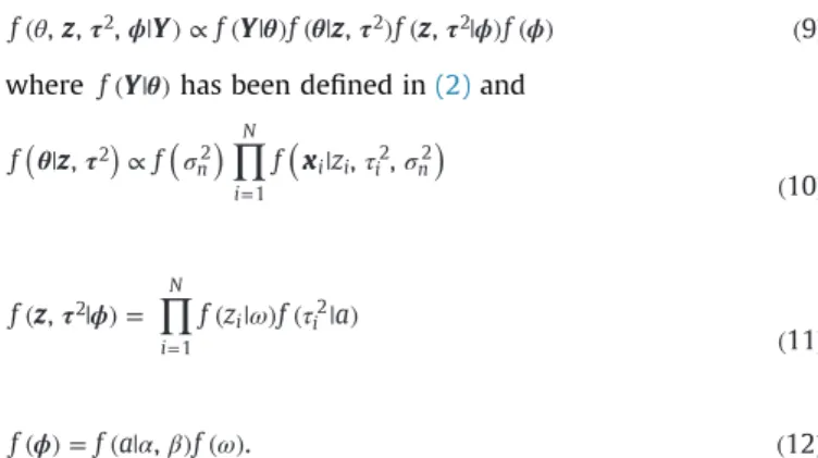
Using the previously described priors and hyperpriors, the posterior distribution of the proposed Bayesian model is
τ ϕ θ θ τ τ ϕ ϕ
θ
( z | ) ∝ ( | ) ( |Y Y z ) (z | ) ( ) ( )
f , , 2, f f , 2f , 2 f 9
where f( | )Yθ has been defined in(2)and
( )
(
)
(
θ| τ)
∝ σ∏
| τ σ ( ) = z x f , f f z, , 10 n i N i i i n 2 2 1 2 2∏
τ ϕ ω τ ( | ) = ( | ) ( | ) ( ) = z f , f z f a 11 i N i i 2 1 2 ϕ α β ω ( ) = ( | ) ( ) ( ) f f a , f . 12The posterior distribution(9)is intractable and does not allow us to derive closed-form expressions for the Bayesian estimators of the different parameters and hyperparameters. Thus we propose to draw samples from(9)and use them to estimate the brain ac-tivity jointly with the model hyperparameters. The following section provides more details about the sampling method in-vestigated in this paper.
3. A partially collapsed Gibbs sampler
We investigate a partially collapsed Gibbs sampler that samples the variables ziandxijointly. IfX−idenotes the matrixXwhose ith
row has been replaced by zeros, the resulting sampling strategy is summarized in Algorithm 1. The corresponding conditional dis-tributions are described inAppendix B.
Algorithm 1. Partially Collapsed Gibbs sampler. Initialize X=0and z=0
Sample a and
τ
2from their prior distributionsrepeat Sample sn2from f
(
σn2|Y X, ,τ2,z)
Sampleω
from f( | )ωz for i¼1 to N do Sampleτ
i2from f(
τi2|xi,σn2, ,a zi)
Sample zifrom f z(
i|Y X, −i,σn2,τi2,ω)
Sample xifrom f(
xi|z ,i Y X, −i,σn2,τi2)
end for Sample a from f a( )
|τ2 until convergence3.1. Multiple dipole shift proposals
The partially collapsed Gibbs sampler summarized in Algo-rithm 1may get stuck around local maxima of the variablezfrom which it can be difficult to escape in a reasonable amount of iterations (examples illustrating this situation are shown inCosta et al., 2015). In order to bypass this problem, we introduce specific Metropolis–Hastings moves. These moves consist of proposing a new value of z (referred to as “candidate”) after each sampling iteration. The candidate is then accepted or rejected with an ap-propriate acceptance rate according to the Metropolis–Hastings rule, which guarantees that the target distribution is preserved.
Before presenting the proposal scheme, it is interesting to mention that it was inspired by an idea developed inBourguignon and Carfantan (2005). The authors ofBourguignon and Carfantan (2005)proposed to move a random non-zero element of a binary sequence to a random neighboring position after each iteration of the MCMC sampler. We have generalized their scheme by pro-posing to move a random subset of K estimated non-zeros si-multaneously to random neighboring positions. According to ex-perimental results (some of them described in Section 4), the simple choice K¼2 provides good results in most practical cases. Since there is a high correlation between the variables
τ
2andz, itis convenient to update their values jointly. The resulting proposal is shown inAlgorithm 2where
(
z τ |Y σ ω)
∝(
−ω)
ω( )
σ − | |Σ ( ) f r, r , ,a n, 1 13 C C n TC T 2 2 2 2 2 0 1 1 ⎛ ⎝ ⎜ ⎜ ⎞ ⎠ ⎟ ⎟ ⎛ ⎝ ⎜ ⎜ ⎞ ⎠ ⎟ ⎟∏
( )τ −∑∏
τ + ( ) ∈ − = = K T v a exp 2 1 2 , 2 . 14 I i i T tT t i N i i 2 2 1 1 2 1 .Algorithm 2. Multiple dipole shift proposal.
¯ =
z z
repeat K times
Setindoldto be the index of a random non-zero of z
Set p= [indold, neigh indγ( old)]
Fig. 1. Directed acyclic graph for the Bayesian model illustrating the dependencies between the model parameters and hyperparameters.
Set indnewto be a random element of p
Set z¯indold=0and z¯indnew=1
end
Sample X¯ from f
(
X z Y¯ |¯, ,σn2,τ2)
. Sampleτ¯2from f(
τ¯ | ¯X,σ , ,a z¯)
n
2 2 .
Set{z,τ2} = { ¯ ¯ }z,τ2 with probability
(
τ)
τ ( ¯ ¯ | ) ( | ) min z , 1 z f f , . , . 2 2Resample X if the proposal was accepted
wherer= {i z: i≠ ¯ }zi ,Ik= {i z: ri= }k andCk=# Ikfork= {0, 1}and
⎡ ⎣ ⎢ ⎢ ⎛ ⎝ ⎜ ⎞ ⎠ ⎟ ⎤ ⎦ ⎥ ⎥ Σ σ τ = ( ) + ( ) − 1 H H diag 1 15 I I r n T 1 2 1 1 2 μ Σ σ = − ( ) ( − ) ( ) − − H H x y 16 I r r t T t t n2 1 σ μ Σ μ = ( − ) ( − ) − ( ) − − − − − H x y H x y K . 17 r r r r t t t T t t n t T t 2 1
Note that m−sdenotes the vector m whose rows belonging to s
have been removed, M−s is the matrix M whose columns
be-longing to s have been removed, diag( )s is the diagonal square matrix whose diagonal elements are the elements ofs and| |M is the determinant of the matrix M.
Algorithm 2also uses the following neighborhood definition
{
γ}
( ) ≜ ≠ | ( )| ≥ ( )
γ i j i h h
neigh corr i, j 18
wherecorr(v v1, 2)is the correlation between vectorsv1andv2. The
neighborhood size can be adjusted by setting γ∈ [0, 1] (γ= 0
corresponds to a neighborhood containing all the dipoles andγ= 1
corresponds to an empty neighborhood). To maximize the moves efficiency, the value of
γ
has to be selected carefully. Experiments during this study have shown that a good compromise is obtained with γ= 0.8. A comparison of the results obtained with and without multiple dipole shift proposals can be found inCosta et al. (2015).3.2. Inter-chain proposal
Another possibility to improve the convergence speed of the proposed partially collapsed Gibbs sampler is to run multiple MCMC chains in parallel and exchange some information between them. Several methods have already been explored to perform this “exchange of information”, including Metropolis-coupled MCMC (Geyer, 1991), Population MCMC (Laskey and Myers, 2003) and simulated tempering (Geyer and Thompson, 1995;Marinari and Parisi, 1992). In this paper, we introduce inter-chain moves by proposing to exchange the values of zand τ2between different
chains. This exchange is accepted with the probability shown in
Algorithm 3. Note that “a between-chain exchange” is made after each iteration with probability p (adjusted to 1
1000 by cross
vali-dation) according to Algorithm 3. A comparison of the results obtained with and without these inter-chain proposals can be found inCosta et al. (2015).
Algorithm 3. Inter-chain proposals.
Define a vectorc= {1, 2,… },L where L is the number of chains fori= {1, 2,… },L
Choose (and remove) a random element fromcand denote it
by k
Denote as{ ¯ ¯ }z ,k τk2 the sampled values of{z,τ2}of MCMC
chain number#k
For the chain#iset{zi,τi2} = { ¯ ¯ }zk,τk2 with probability τ τ ( ¯ ¯ | ) ( | ) z z f f , . , . k k2 2
Resample X if the proposal has been accepted end
3.3. Estimators
The point estimators used in this study are defined as
(
)
^ ≜ ¯ ∈{ } # (¯) ( ) z arg maxz 0,1N 4 z 19∑
^ ≜ # (^) ∈ (^) ( ) ( ) z p 1 p 20 z m m 4 4where 4( ¯)z is the set of iteration numbers m for which z( )m = ¯z
after the burn-in period and p( )m is the m-th sample of
{
σ ω τ}
∈ > X
p , ,a n2, , 2 . Thus the estimator ^zin (19)is the
max-imum a posteriori estimator of ^zwhereas the estimator used for all the other sampled variables in (20) is the minimum mean square error (MMSE) estimator.
It is interesting to note that the proposed method does not only provide point-estimators as the methods based on the ℓ21mixed
norm. For instance, in some cases different values ofzcan have a significant posterior probability. In this case the sampler may os-cillate between different values of z that usually differ by minor variations. In these cases, the proposed sampling method is able to identify several possible solutions (each of them corresponding to a different value of z) with their corresponding probabilities.
4. Experimental results
4.1. Synthetic data
Synthetic data are first considered to compare the ℓ21 mixed
norm approach, the Champagne model and the proposed method using a 212-dipole Stok three-sphere head model (Stok, 1986) with 41 electrodes. Two kinds of activations are considered: (1) three dipoles with low SNR and (2) multiple dipoles with high SNR. Note that additional experiments are available in the associated tech-nical report (Costa et al., 2015).
4.1.1. Three-dipoles with low SNR
Three dipoles were assigned damped sinusoidal excitations with frequencies varying between 5 and 20 Hz. These excitations were 500 ms long (a period corresponding to a stationary dipole activity) and sampled at 200 Hz. Different levels of noise were used to compare the performance of the different methods. The parameters of the proposed multiple dipole shift proposal were set to K¼2, γ= 0.8and C¼8 MCMC chains were run in parallel. The potential scale reduction factor (PSRF) (Gelman and Rubin, 1992) was used to assess the convergence of the proposed method. After running a fixed number of 10,000 iterations, the PSRFs of all the sampled variables were computed and we checked that these values were below 1.2 as recommended in (Gelman et al., 1995p. 332). For the ℓ21mixed norm approach, the value of the
regular-ization parameter
λ
was chosen using cross-validation.For high values of the input SNR (≥20 dB), the results obtained with all methods are almost always identical to the ground truth. However, for lower values of SNR the proposed method outperforms
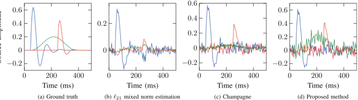
the other two. The estimated dipole locations associated with SNR¼−3 dBare shown inFig. 2and the corresponding estimated waveforms in Fig. 3. Fig. 4 shows the ground truth of the three waveforms compared to the μ± 2σ boundaries estimated by the proposed method. Note that only the dipoles with highest activity are displayed for the ℓ21approach. The approach based on the ℓ21
norm manages to recover only two of the three non-zero activities at the correct positions and seems to underestimate considerably the amplitude of this activity. This is a known problem caused by ap-proximating the ℓ0pseudo-norm by the ℓ1norm. In comparison, the
Champagne method spreads the activity of some of the active di-poles to its neighbors. The proposed algorithm oscillates between several values of z(specified inTable 1). However, the most prob-able value ofzfound by the algorithm is the correct one whereas the other most likely values ofzhave one of the non-zeros moved to a close neighbor. Finally, the histograms of the hyperparameters generated by the proposed Gibbs sampler are displayed in Fig. 5, showing a good agreement with the actual values of the parameters
ω
and sn2and allowing the parameter a associated with the latentvariables
τ
i2to be estimated.Fig. 2. Results for synthetic data with three active dipoles and low SNR: Comparison between the ground truth positions of the active dipoles with the positions estimated by different algorithms. The proposed method is the only one to find all dipoles in the correct places (a) Ground truth - Axial, coronal and sagittal views respectively, (b) Weighted ℓ21- Axial, coronal and sagittal views respectively, (c) Champagne - Axial, coronal and sagittal views respectively, (d) Proposed method - Axial, coronal and sagittal views respectively.
To conclude, the proposed method improves the EEG source localization thanks to the use of a Laplace Bernoulli prior. More-over, the use of an MCMC method makes it possible to recover different sets of source locations with their respective probabilities.
4.1.2. Multiple dipoles
In each simulation of this section, P dipoles were activated with damped sinusoidal waves whose frequencies vary between 5 and 20 Hz. The activations were sampled at 200 Hz and scaled in amplitude so that each of them produced the same energy in the measurements. Fifty different sets of localizations were used for the active dipole positions for each value ofP=1,…, 20, resulting in a total of 1000 experiments. Noise was added to the measure-ments to obtain SNR ¼30 dB. For the ℓ21mixed norm
regulariza-tion the regularizaregulariza-tion parameter was set according to the un-certainty principle which consists in finding a solutionX^such that
∥HX^ − ∥ ≈ ∥Y HX−Y∥(Morozov, 1966).
For each simulation, the estimated activity was defined as the P dipoles that had the highest value of x
v
i i
2
2 . The other dipoles were
considered as residuals. We define the recovery rate as the pro-portion of active dipoles in the ground truth that are also present in the estimated activity. The average recovery rates of the Fig. 3. Results for synthetic data with three active dipoles and low SNR: Comparison between the ground truth and the waveforms estimated by different algorithms. The estimates obtained with the proposed method are closer to the ground truth (a) Ground truth, (b) ℓ21mixed norm estimation, (c) Champagne, (d) Proposed method.
Fig. 4. Results for synthetic data with three active dipoles and low SNR: Ground truth activation waveforms compared withμ± 2σboundaries estimated by the proposed method. The ground truth waveforms are within the estimated boundaries (a) Dipole waveform 1, (b) Dipole waveform 2, (c) Dipole waveform 3.
Table 1
Results for synthetic data with three active dipoles and low SNR: modes explored by the proposed algorithm. Positions 1, 2 and 3 correspond to the non-zero ele-ments of the ground truth, showing that the ground truth mode is the most ex-plored mode after convergence.
Active non-zeros Percentage of samples
1 2 3 43 1 2 4 22 1 2 5 11 1 2 6 7 1 2 7 6 Others 11
Fig. 5. Results for synthetic data with three active dipoles with low SNR: histograms of the hyperparameters by the proposed method after convergence. The actual values of ωand sn2are marked with a red vertical line, showing close values to the ones sampled by the algorithm (a) Histogram of ω, (b) Histogram of a, (c) Histogram of sn2.
proposed method and the ℓ21mixed norm approach are presented
inFig. 6a as a function of P. For P≤10, the proposed algorithm detects the non-zeros with an accuracy higher than 90% which drops to 60.2% for P¼11 and 49.7% for P¼12. This drop of the recovery rate when a large number of non-zeros is present in the ground truth is well known, since the possible amount of non-zeros to recover correctly is limited by the operator span (Candes, 2008). For comparison, the ℓ21 mixed norm regularization
re-covers up to P¼5 non-zeros with an accuracy higher than 90% and its recovery rate decreases slowly to reach 64% for P¼10. Note that the proposed method has a higher recovery rate than the ℓ21
ap-proach forP≤11. Beyond this point, the poor performance of both methods prevents them from being used in real applications.
It is also interesting to analyze how much activity is present in the residual non-zeros. Thus, we define the proportion of residual energy as the amount of energy contained in the measurements generated by the residual non-zeros with respect to the total energy in the measure-ments.Fig. 6b shows the value of the residual energy obtained for both algorithms as a function of P. The ℓ21approach has up to 7.7% of the
activity detected in residual non-zeros whereas the proposed algorithm algorithm never exceeds 1.1%, confirming its good sparsity properties.
4.2. Real data
Two real data sets are considered in this section. The first data set corresponds to the auditory evoked responses to left ear pure tone stimulus while the second one consists of the evoked re-sponses to facial stimulus. The results of the proposed method are compared with the weighted ℓ21 mixed norm (Gramfort et al., 2012), the Champagne model (Wipf et al., 2010) and the method investigated inFriston et al. (2008)based on multiple sparse priors.
4.2.1. Auditory evoked responses
The default data set of the MNE software (Gramfort et al., 2014,
2013) is used in this section. It consists of the evoked response to left-ear auditory pure-tone stimulus using a realistic BEM (Bound-ary element method) head model sampled with 60 EEG electrodes and 306 MEG sensors. The head model contains 1.844 dipoles lo-cated on the cortex with orientations that are normal to the brain surface. Two channels that had technical artifacts were ignored. The data was sampled at 600 Hz. The samples were low-pass filtered at 40 Hz and downsampled to 150 Hz. The noise covariance matrix was estimated from 200 ms of the data preceding each stimulus and was used to whiten the measurements. Fifty-one epochs were averaged to calculate the measurements Y. The activity of the source dipoles was estimated jointly for the period from 0 ms to 500 ms after the stimulus. It is expected to find the brain activity primarily focused on the auditory cortices that are located close to the ears in both hemispheres of the brain (Gramfort et al., 2012).
The uncertainty principle was used to adjust the hyperparameter of the ℓ21mixed norm leading to having activity distributed all over
the brain as shown in Fig. 7(a). By manually adjusting the
hyperparameter to produce a sparser result, it is possible to obtain a solution that has activity in the auditory cortices as shown inFig. 7(b). In contrast, the proposed algorithm estimates its hyperparameters automatically and finds most of the activity in the auditory cortices without requiring any manual adjustment. The MSP method also finds the activity in both auditory cortices whereas the Champagne model finds an active patch on one of them. In addition,Fig. 8shows the estimated waveforms using the ℓ21mixed norm and the proposed
method. As we can see, they both have sharp peaks between 80 and 100 ms after the application of the stimulus, as expected in the re-sponse to an auditory stimulus (Gramfort et al., 2012).
To summarize, the proposed method finds the EEG source ac-tivity in areas that are spatially coherent with those found by the MSP and the Champagne methods. The main difference between the results is that the proposed method estimates the brain activity to be in only a few dipoles whereas the other algorithms estimate its extent. This is due to the sparsity-promoting prior that focuses the brain activity on the most important sources. Note that more details about the experiment are available inCosta et al. (2015).
4.2.2. Facial evoked responses
In a second step, data acquired from a face perception study where the subject was required to evaluate the symmetry of a mixed set of faces and scrambled faces was used, one of the default data sets of the SPM software.2 Faces were presented during 600 ms every 3600 ms. The measurements were obtained by the electrodes of a 128-channel ActiveTwo system with a sampling frequency of 2048 Hz. The measurements were downsampled to 200 Hz and, after artifact rejection, 299 epochs corresponding to the non-scrambled faces were averaged and low-pass filtered to 40 Hz. A T1 MRI scan was then downsampled to generate a 8196 dipole head model.
The estimated activities are shown inFig. 9. Using the proposed method, one can note that the activity is localized close to the fusiform region in the occipital lobe (Kanwisher et al., 1997). This in good agreement with the results obtained by the MSP and Champagne algorithms. Again, the difference is related to the fo-calization of the activity among a reduced number of dipoles.
4.3. Computational cost
It is important to note that the price paid for the proposed method, while having several advantages over the ℓ21mixed norm
approach, is its higher computational complexity. This problem is typical with MCMC methods when compared to optimization techniques. More precisely, the low SNR three-dipole experiment was processed in 6 s using a modern Xeon CPU E3-1240 @ 3.4 GHz processor (and a Matlab implementation with MEX files written in C) against 104 ms for the ℓ21mixed norm approach. However, it is
interesting to note that the ℓ21 norm approach requires running
Fig. 6. Results for synthetic data with multiple active dipoles: Performance as a function of the amount of active dipoles (P).
Fig. 7. Results for real data auditory evoked responses: Active dipole positions estimated by different algorithms. The proposed method finds the activity focused in both auditory cortices as the MSP algorithm does. The Champagne model finds the activity in one of the auditory cortices (a) Weighted ℓ21norm - Uncertainty principle for parameter λ, (b) Weighted ℓ21norm - Manual adjustment of parameter λ, (c) Proposed method, (d) MSP algorithm, (e) Champagne.
the algorithm multiple times to adjust the regularization parameter.
5. Conclusion
We presented a Bayesian mathematical model for sparse EEG
reconstruction that approximates the ℓ20mixed norm in a
Baye-sian framework by a multivariate Bernoulli Laplacian prior. A partially collapsed Gibbs sampler was used to sample from the target posterior distribution. We introduced multiple dipole shift proposals within each MCMC chain and exchange moves between different chains to improve the convergence speed. Using the generated samples, the source activity was estimated jointly with the model hyperparameters in an unsupervised framework. The proposed method was compared with the ℓ21 mixed norm, the
Champagne algorithm and a method based on multiple sparse priors in a wide variety of situations including several multi-dipole synthetic activations and two different real data sets. Using syn-thetic data sets, the proposed algorithm presented several ad-vantages including better recovery of dipole locations and wave-forms in low SNR conditions, the capacity of correctly detecting a higher amount of non-zeros, providing sparser solutions and avoiding underestimation of the activation amplitude. Using the real data sets, the proposed algorithm finds activity in locations that are spatially coherent with those found by the MSP and the Champagne algorithms. Finally, the possibility of providing several solutions with their corresponding probabilities is interesting. Future work will be devoted to a generalization of the proposed model to cases where the head model is not precisely known. Possible future options are to extend the current work to run Fig. 8. Estimated waveforms for real data auditory evoked responses: Measurements
and estimated activation waveforms. Both algorithms find the peak activity around 90ms after the stimulus was applied as expected (a) Weighted ℓ21norm, (b) Proposed method.
Fig. 9. Results for facial evoked responses: Active dipole positions estimated by different algorithms. The proposed method finds the activity in locations that are compatible with the ones estimated by the Champagne and MSP algorithms (a) Proposed method, (b) MSP algorithm, (c) Champagne.
models for estimating the spread patterns of the activity in epilepsy.
Acknowledgement
This work is part of the DynBrain project funded by STIC-AM-SUD in collaboration with ITBA (Buenos Aires) and the FLENI hospital (Buenos Aires).
The authors would also like to thank Professor Steve McLaughlin from Heriot Watt University for improving the read-ability of the paper.
Appendix A. Parameter priors
In this appendix the priors that were used for the variance of the noise sn2and the hyperparameters a and
ω
are detailed.A.1. Noise variance activity sn2
The noise variance is assigned a Jeffrey's prior
5
( )
σ( )
σ σ ∝ ( ) + f 11 21 n n n 2 2 2where 15+( ) =ξ 1if ξ∈5+ and 0 otherwise. This choice is very
classical when no information about a scale parameter is available (seeCasella and Robert, 1999for details).
A.2. Hyperprior of a
A conjugate gamma prior is assigned to a
(
)
α β α β
( | ) = ( )
f a , . a , 22
with α=β= 1. These values of
α
andβ
yield a vague hyperprior for a. The conjugacy of this hyperprior will make the analysis easier.A.3. Hyperprior of
ω
A uniform prior on [0, 1] is used for
ω
ω ω
( ) = [ ]( ) ( )
f <0,1 23
reflecting the absence of knowledge for this hyperparameter.
Appendix B. Conditional distributions
The conditional distributions of the model parameters used in
Algorithm 1are detailed below.
B.1. Conditional distribution of
τ
i2The conditional distribution of
τ
i2 is a gamma (.) or agen-eralized inverse Gaussian (.0.) distribution depending on the value of zi. More precisely
⎧ ⎨ ⎪ ⎪ ⎩ ⎪ ⎪ ⎛ ⎝ ⎜ ⎞ ⎠ ⎟ ⎛ ⎝ ⎜⎜ ⎞ ⎠ ⎟⎟
(
τ σ)
τ τ σ | = + = ∥ ∥ = ( ) x x f a z T v a z v a z , , , 1 2 , 2 if 0 1 2, , if 1. 24 i i n i i i i i i i n i 2 2 2 2 2 2 . .0. B.2. Conditional distribution of xiThe conditional distribution of the ith row of X is
⎧ ⎨ ⎪ ⎩ ⎪
(
)
(
σ τ)
μ δ σ | = ( ) = = ( ) − x Y X x x f z z z , , , , if 0 , if 1 25 i i i n i i i i i i i 2 2 2 5 with μ σ σ σ σ τ τ = ( − ) = + ( ) − h Y HX h h , 1 . 26 i i iT i n i n i i iT i 2 2 2 2 2 2 B.3. Conditional distribution of ziThe conditional distribution of ziis a Bernoulli distribution
⎛ ⎝ ⎜ ⎞ ⎠ ⎟
(
| σ τ ω)
= + ( ) − Y X f z z k k k , , , , 1, 27 i i n2 i2 i 1 0 1 ) with ⎛ ⎝ ⎜ ⎞ ⎠ ⎟ ⎛ ⎝ ⎜ ⎜ ⎞ ⎠ ⎟ ⎟ μ ω ω σ τ σ σ = − = ∥ ∥ ( ) − k 1 , k exp 2 . 28 n i i T i i 0 1 2 2 2 2 2 2 B.4. Conditional distribution of aThe conditional distribution of a|τ2 is the following gamma
distribution ⎛ ⎝ ⎜ ⎜ ⎞ ⎠ ⎟ ⎟ τ α τ β ( | ) = ( + ) + ∑ + ( ) = f a a N T 1 v 2 , 2 . 29 i N i i 2 1 2 . B.5. Conditional distribution of sn2
The distribution ofσn2|Y X, ,τ2,zis the following inverse gamma (0.) distribution ⎛ ⎝ ⎜ ⎜ ⎡ ⎣ ⎢ ⎢ ⎤ ⎦ ⎥ ⎥ ⎞ ⎠ ⎟ ⎟
∑
σ τ ( + ∥ ∥ ) ∥ − ∥ + ∥ ∥ ( ) = z HX Y x M T 2 , 1 2 . 30 n i N i i 2 0 2 1 2 2 0. B.6. Conditional distribution ofω
Finally,ω|zhas the following beta distribution
(
)
ω ω
( | ) =z + ∥ ∥z + − ∥ ∥z ( )
f )e 1 0, 1 N 0. 31
References
Berg, A.T., Berkovic, S.F., Brodie, M.J., Buchhalter, J., Cross, J.H., van Emde Boas, W., Engel, J., French, J., Glauser, T.A., Mathern, G.W., et al., 2010. Revised termi-nology and concepts for organization of seizures and epilepsies: report of the ILAE Commission on Classification and Terminology, 2005-2009. Epilepsia 51 (4), 676–685.
Bourguignon, S., Carfantan, H.,Jul. 2005. Bernoulli-Gaussian spectral analysis of unevenly spaced astrophysical data. In: Proceedings of the IEEE Workshop on Statistical Signal Processing (SSP), Bordeaux, France.
Candes, E.J., 2008. The restricted isometry property and its implications for com-pressed sensing. C. R. Acad. Sci. 346 (9), 589–592.
Casella, G., Robert, C.P., 1999. Monte Carlo Statistical Methods. Springer-Verlag, New York.
Castaño-Candamil, S., Höhne, J., Martínez-Vargas, J.-D., An, X.-W., Castellanos-Domínguez, G., Haufe, S., 2015. Solving the EEG inverse problem based on space-time-frequency structured sparsity constraints. NeuroImage 118, 598–612.
Bayesian particle filtering. In: Proceedings of the IEEE International Conference on Acoustics, Speech, Signal Processing (ICASSP), Vancouver, Canada. Costa, F., Batatia, H., Oberlin, T., Tourneret, J.-Y., 2015. Bayesian Structured Sparsity
Priors for EEG Source Localization Technical Report. University of Toulouse, ENSEEIHT, Technical Report. [Online]. Available: http://arxiv.org/abs/1509. 04576.
Costa, F., Batatia, H., Chaari, L., Tourneret, J.-Y., 2015. Sparse EEG source localization using Bernoulli Laplacian priors. IEEE Trans. Biomed. Eng. 62 (12), 2888–2898. da Silva, F.L., Van Rotterdam A., Biophysical aspects of EEG and magnetoencepha-logram generation. In: Electroencephalography: Basic Principles, Clinical Ap-plications and Related Fields. Williams & Wilkins, Baltimore.
Friston, K., Harrison, L., Daunizeau, J., Kiebel, S., Phillips, C., Trujillo-Barreto, N., Henson, R., Flandin, G., Mattout, J., 2008. Multiple sparse priors for the M/EEG inverse problem. NeuroImage 39 (3), 1104–1120.
Galka, A., Yamashita, O., Ozaki, T., Biscay, R., Valdés-Sosa, P., 2004. A solution to the dynamical inverse problem of EEG generation using spatiotemporal Kalman filtering. NeuroImage 23 (2), 435–453.
Gelman, A., Rubin, D.B., 1992. Inference from iterative simulation using multiple sequences. Stat. Sci. 7 (4), 457–511.
Gelman, A., Carlin, J.B., Stern, H.S., Rubin, D.B., 1995. Bayesian Data Analysis. Chapman & Hall, London, UK.
Geyer, C.J., Thompson, E.A., 1995. Annealing Markov chain Monte Carlo with ap-plications to ancestral inference. J. Am. Stat. Soc. 90 (431), 909–920. Geyer, C.J., Oct. 1991. Markov chain Monte Carlo maximum likelihood. In:
Pro-ceedings of the 23rd Symposium on Interface Computer Science and Statistics, Seattle, USA.
Gramfort, A., Kowalski, M., Hämäläinen, M., 2012. Mixed-norm estimates for the M/ EEG inverse problem using accelerated gradient methods. Phys. Med. Biol. 57 (7), 1937.
Gramfort, A., Luessi, M., Larson, E., Engemann, D.A., Strohmeier, D., Brodbeck, C., Goj, R., Jas, M., Brooks, T., Parkkonen, L., et al., 2013. MEG and EEG data analysis with MNE-Python. Front. Neurosci. 7 (267), 1–13.
Gramfort, A., Strohmeier, D., Haueisen, J., Hämäläinen, M.S., Kowalski, M., 2013. Time-frequency mixed-norm estimates: sparse M/EEG imaging with non-sta-tionary source activations. NeuroImage 70, 410–422.
Gramfort, A., Luessi, M., Larson, E., Engemann, D.A., Strohmeier, D., Brodbeck, C., Parkkonen, L., Hämäläinen, M.S., 2014. MNE software for processing MEG and EEG data. NeuroImage 86, 446–460.
Grech, R., Cassar, T., Muscat, J., Camilleri, K.P., Fabri, S.G., Zervakis, M., Xanthopoulos, P., Sakkalis, V., Vanrumste, B., 2008. Review on solving the inverse problem in EEG source analysis. J. Neuroeng. Rehabil. 4, 5–25.
Hallez, H., Vanrumste, B., Grech, R., Muscat, J., De Clercq, W., Vergult, A., D'Asseler, Y., Camilleri, K.P., Fabri, S.G., Van Huffel, S., et al., 2007. Review on solving the forward problem in EEG source analysis. J. Neuroeng. Rehabil. 4, 46–75. Huang, J., Zhang, T., 2010. The benefit of group sparsity. Ann. Stat. 38 (August (4)),
1978–2004.
Huang, J., Zhang, T., Metaxas, D., 2011. Learning with structured sparsity. J. Mach. Learn. Res. 12, 3371–3412.
Kanwisher, N., McDermott, J., Chun, M.M., 1997. The fusiform face area: a module in human extrastriate cortex specialized for face perception. J. Neurosci. 17 (11), 4302–4311.
Kowalski, M., Siedenburg, K., Dorfler, M., 2013. Social sparsity! Neighborhood sys-tems enrich structured shrinkage operators. IEEE Trans. Signal Process. 61 (10), 2498–2511.
Lamus, C., Hämäläinen, M.S., Temereanca, S., Brown, E.N., Purdon, P.L., 2012. A spatiotemporal dynamic distributed solution to the MEG inverse problem. NeuroImage 63 (2), 894–909.
Laskey, K.B., Myers, J.W., 2003. Population Markov chain Monte Carlo. Mach. Learn. 50, 175–196.
Long, C.J., Purdon, P.L., Temereanca, S., Desai, N.U., Hämäläinen, M.S., Brown, E.N., 2011. State-space solutions to the dynamic magnetoencephalography inverse
problem using high performance computing. Ann. Appl. Stat. 5 (2B), 1207–1228.
Lucka, F., Pursiainen, S., Burger, M., Wolters, C., 2012. Hierarchical Bayesian in-ference for the EEG inverse problem using realistic FE head models: depth localization and source separation for focal primary currents. NeuroImage 61 (april (4)), 1364–1382 [Online]. Available: /2012/LPBW12.
Marinari, E., Parisi, G., 1992. Simulated tempering: a new Monte Carlo scheme. Europhys. Lett. 19 (6), 451–458.
Maris, E., 2003. A resampling method for estimating the signal subspace of spatio-temporal EEG/MEG data. IEEE Trans. Biomed. Eng. 50 (8), 935–949. Morozov, V.A., 1966. On the solution of functional equations by the method of
regularization. Sov. Math. Dokl. 7, 414–417.
Pascual-Marqui, R.D., Michel, C.M., Lehmann, D., 1994. Low resolution electro-magnetic tomography: a new method for localizing electrical activity in the brain. Int. J. Psychophysiol. 18 (1), 49–65.
Pascual-Marqui, R., et al., 2002. Standardized low-resolution brain electromagnetic tomography (sLORETA): technical details. Methods Findings Exp. Clin. Phar-macol. 24D, 5–12.
Pascual-Marqui, R.D., 1999. Review of methods for solving the EEG inverse problem. Int. J. Bioelectromagn. 1 (1), 75–86.
Quintero-Rincón, A., Pereyra, M., DGiano, C., Batatia, H., Risk, M., 2016. A new al-gorithm for epilepsy seizure onset detection and spread estimation from eeg signals. In: Journal of Physics: Conference Series, vol. 705, no. 1. IOP Publishing, San Nicolás de los Arroyos, Argentina, p. 012032.
Raman, S., Fuchs, T.J., Wild, P.J., Dahl, E., Roth, V., Jun. 2009. The Bayesian group-lasso for analyzing contingency tables.” In: Proceedings of the 26th ACM Annual International Conference on Machince Learning (ICML), Montreal, Quebec. Somersalo, E., Voutilainen, A., Kaipio, J., 2003. Non-stationary
magnetoencephalo-graphy by Bayesian filtering of dipole models. Inv. Probl. 19 (5), 1047–1063. Sommariva, S., Sorrentino, A., 2014. Sequential Monte Carlo samplers for
semi-linear inverse problems and application to magnetoencephalography. Inv. Probl. 30 (11), 114 020–114 043.
Sorrentino, A., Johansen, A.M., Aston, J.A., Nichols, T.E., Kendall, W.S., et al., 2013. Dynamic filtering of static dipoles in magnetoencephalography. Ann. Appl. Stat. 7 (2), 955–988.
Stahlhut C., Attias, H.T., Sekihara, K., Wipf, D., Hansen, L.K., Nagarajan, S.S., 2013. A hierarchical Bayesian M/EEG imaging method correcting for incomplete spatio-temporal priors. In: Proceedings of the IEEE 10th International Symposium on Biomedical Imaging (ISBI), San Francisco, USA, April.
Stok, C.J., 1986. The Inverse Problem in EEG and MEG with Application to Visual Evoked Responses,” Ph.D. dissertation, University of Twente, Enschede, The Netherlands.
Strohmeier, D., Haueisen, J., Gramfort, A., Improved MEG/EEG source localization with reweighted mixed-norms. 2014. In: Proceedings of the 4th International Workshop on Pattern Recognition in Neuroimaging 2014 (PRNI 2014). IEEE, Tübingen, Germany, pp. 1–4.
Uutela, K., Hämäläinen, M., Somersalo, E., 1999. Visualization of magnetoence-phalographic data using minimum current estimates. NeuroImage 10 (2), 173–180.
Wipf, D.P., Owen, J.P., Attias, H.T., Sekihara, K., Nagarajan, S.S., 2010. Robust Bayesian estimation of the location, orientation, and time course of multiple correlated neural sources using MEG. NeuroImage 49 (1), 641–655.
Yu, G., Sapiro, G., Mallat, S., 2012. Solving inverse problems with piecewise linear estimators: from Gaussian mixture models to structured sparsity. IEEE, Tü-bingen, Germany, Trans. Image Process. 21 (5), 2481–2499.
Yuan, M., Lin, Y., 2006. Model selection and estimation in regression with grouped variables. J. R. Stat. Soc. 68 (1), 49–67.
Zhang, Z., Rao, B.D., 2011. Sparse signal recovery with temporally correlated source vectors using sparse Bayesian learning. IEEE J. Sel. Topics. Signal Process. 5 (5), 912–926.