Any correspondence concerning this service should be sent
to the repository administrator: [email protected]
This is an author’s version published in:
http://oatao.univ-toulouse.fr/22715
Official URL
DOI : https://doi.org/10.4230/LIPIcs.FSCD.2016.14
Open Archive Toulouse Archive Ouverte
OATAO is an open access repository that collects the work of Toulouse
researchers and makes it freely available over the web where possible
To cite this version:
Brenas, Jon Haël and Echahed, Rachid and Strecker,
Martin Proving Correctness of Logically Decorated Graph Rewriting
Systems. (2016) In: 1st International Conference on Formal Structures for
Computation and Deduction (FSCD 2016), 22 June 2016 - 26 June 2016
(Porto, Portugal).
Proving Correctness of Logically Decorated Graph
Rewriting Systems
∗
Jon Haël Brenas
1, Rachid Echahed
2, and Martin Strecker
31 CNRS and Université Grenoble Alpes, Saint Martin d’Hères, France [email protected]
2 CNRS and Université Grenoble Alpes, Saint Martin d’Hères, France [email protected]
3 IRIT – Université de Toulouse, Toulouse, France [email protected]
Abstract
We first introduce the notion of logically decorated rewriting systems where the left-hand sides are endowed with logical formulas which help to express positive as well as negative application conditions, in addition to classical pattern-matching. These systems are defined using graph structures and an extension of combinatory propositional dynamic logic, CPDL, with restricted universal programs, called C2PDL. In a second step, we tackle the problem of proving the correctness of logically decorated graph rewriting systems by using a Hoare-like calculus. We introduce a notion of specification defined as a tuple (Pre, Post, R, S) with Pre and Post being formulas of C2PDL, R a rewriting system and S a rewriting strategy. We provide a sound calculus which infers proof obligations of the considered specifications and establish the decidability of the verification problem of the (partial) correctness of the considered specifications.
Keywords and phrases Graph Rewriting, Hoare Logic,Combinatory PDL, Rewrite Strategies, Program Verification
Digital Object Identifier 10.4230/LIPIcs.FSCD.2016.14
1
Introduction
Rewriting techniques and particularly term rewriting systems have been very successful in different areas such as theorem proving or declarative programming languages. Term rewriting systems have a wide range of interesting results such as confluence analysis, termination orderings and even very powerful proof techniques based, in particular, on equational reasoning and structural induction. However, the structure of terms (trees) is not well suited to specify easily problem handling graph structures, unless one uses cumbersome encodings.
In this paper we will focus on a class of rewriting systems that manipulate graphs. Graphs are data structures that have become ubiquitous. In addition to discrete mathematics and computer science, they are also used to model data in various fields such as biology, geography, physics etc. The transformation of graphs is nowadays a domain of research in its own. One may distinguish two main streams, in the literature, for graph transformations : (i) the algorithmic approaches, which describe explicitly the algorithms involved in the application
∗ This work has been funded by the project CLIMT(ANR/(ANR-11-BS02-016).
© Jon Haël Brenas, Rachid Echahed, and Martin Strecker; licensed under Creative Commons License CC-BY
1st International Conference on Formal Structures for Computation and Deduction (FSCD 2016). Editors: Delia Kesner and Brigitte Pientka; Article No. 14; pp. 14:1–14:15
a00 a01 a02 a03 a10 a11 a12 a13 a20 a21 a22 a23 a30 a31 a32 a33 a00 a01 a02 a03 a10 a11 a12 a13 a20 a21 a22 a23 a30 a31 a32 a33 A B
Figure 1 A – A Sudoku grid. B – An illustration of the correct definition of columns. We omit
the labels of the edges.
of a rule to a graph, and (ii) the algebraic approaches which define abstractly a graph transformation step using basic constructs borrowed from category theory.
In this paper, we follow the algorithmic approach as proposed in [7] and consider rewrite rules of the form lhs → α where lhs is a graph and α is a sequence of elementary actions that perform the desired transformations on the subgraph matched by lhs. We define the notion of logically decorated graph rewriting systems (LDRS) where the left-hand sides of rules are graphs attributed by formulas in a dynamic logic, called C2PDL[5], and whose models are also graphs. Such formulas, within the left-hand sides, could be seen as additional conditions to be fulfilled when matching a subgraph.
After the introduction of LDRS systems, we tackle the problem of their verification with the objective of building a decidable procedure. For that we define a Hoare-like calculus the aim of which is to prove that a transformation is correct, i.e., given a set of rewriting rules, a strategy stating how to apply them, a pre-condition indicating what are the properties to be satisfied before the application of the transformations and a post-condition stating which property is to be verified after the transformations, whether for any graph G satisfying the pre-condition every graph obtained by transforming G will satisfy the post-condition. To do so, we define a calculus that generates weakest-pre-conditions and verification conditions for each intermediate step of the strategy. This infers a weakest pre-condition and a verification condition for the whole transformations. That weakest pre-condition is then compared to the given pre-condition. We show that the proposed Hoare-like calculus is sound and that the considered correctness problem is decidable.
◮ Example 1. To clarify what is our aim and how our system works, we will be using
a running example: we propose to study a simple program dealing with Sudoku grids. For reason of clarity and conciseness, we will study 4x4 grids instead of the normal 9x9. Nonetheless, the example can be easily extended to the normal Sudoku. An example of such a grid is shown in Figure 1.A. The goal is to fill each blank cell with a number between 1 and 4 such that the same number doesn’t appear twice on a line, a column or a square. The goal of this example is not to show that graph transformations are efficient for solving Sudokus but just to provide a rather simple and common example in order to illustrate how to carry out the correctness proof of a program defined as a graph rewrite system.
The paper is organized as follows. In the following section, the dynamic logic C2PDL used to express pre- and post-conditions is presented briefly. Then, the class of logically decorated rewriting systems is defined in Section 3 together with a notion of rewrite strategies. In Section 4, we start by setting the verification problem we consider and show how the proof obligations are generated. We also prove that the presented verification process is sound and decidable. An overview of related work is given in Section 5. Section 6 concludes the paper.
2
The dynamic logic C2PDL
In this section, we introduce C2PDL [5], a logic that we use to specify assertions. It is a mix of Converse Propositional Dynamic Logic [8] and Combinatory Propositional Dynamic Logic [15], both commonly known as CPDL. C2PDL contains elements of Propositional Dynamic Logic, that allows one to define complex role constructors, and Hybrid Logic, which allows one to use the power of nominals. C2PDL further extends the CPDLs in two ways: it splits the universe into elements that are part of the model and elements that may be created by an action or that have been deleted; it also extends the notion of universal role to “total” roles over subsets of the universe in order to be able to deal with these modifications of the universe.
◮Definition 2 (Syntax of C2PDL). Given three countably infinite and pairwise disjoint
alphabets Σ, the set of names, Φ0, the set of atomic propositions, Π0, the set of atomic
programs, the language of C2PDL is composed of formulas and programs1. We partition the set of names Σ into two countably infinite alphabets Σ1and Σ2 such that Σ1∪ Σ2= Σ and Σ1∩ Σ2= ∅. Formulas φ and programs α are defined as:
φ := i| φ0| ¬φ | φ ∨ φ | éαêφ
α := α0| νS| α; α | α ∪ α | α∗| α−| φ?
where i ∈ Σ, φ0∈ Φ0, α0∈ Π0 and S ⊆ Σ.
We denote by Π the set of programs and by Φ the set of formulas. As ususal, φ ∧ ψ stands for ¬(¬φ ∨ ¬ψ) and [α]φ stands for ¬(éαê¬φ).
For now, the splitting of Σ seems artificial. It is actually grounded in the use we want to make of the logic. Roughly speaking, Σ1stands for the names that are used in “the” current model whereas Σ2 stands for the names that may be used in the future (or have been used in the past but do not participate in the current model).
◮Definition 3 (Model). A model is a tuple M = (M, R, χ, V ) where M is a set called the
universe, χ : Σ → M is a surjective mapping such that χ(Σ1) ∩ χ(Σ2) = ∅, R : Π → P(M2) and V : Φ → P(M) are mappings such that:
For each α0∈ Π0, R(α0) ∈ P(χ(Σ1)2) R(νS) = χ(S)2 for S ⊆ Σ R(α ∪ β) = R(α) ∪ R(β) R(A?) = {(s, s)|s ∈ V (A)} R(α−) = {(s, t)|(t, s) ∈ R(α)} R(α∗) =t
k<ωR(αk) where αk stands for the sequence α; . . . ; α of length k
R(α; β) = {(s, t)|∃v.((s, v) ∈ R(α) ∧ (v, t) ∈ R(β))} For each i ∈ Σ, V (i) = {χ(i)}
For each φ0∈ Φ0, V (φ0) ∈ P(χ(Σ1))
V(¬A) = M \V (A)
V(A ∨ B) = V (A) ∪ V (B)
V(éαêA) = {s|∃t ∈ M.((s, t) ∈ R(α) ∧ t ∈ V (A))} In the following, we write sRαtfor (s, t) ∈ R(α).
C2PDL will be used in this paper to label nodes and to express properties of attributed graphs.
1
◮Definition 4 (Attributed Graph). An attributed graph G is a tuple (N ,E,C,R,LN,LE,s,t)
where N is the set of nodes, E is the set of edges, C is the set of node labels or concepts, R is the set of edge labels or roles, LN is the node labeling (total) function, LN : N → P(C), LE
is the edge labeling (total) function, LE: E → R, s is the source function s : E → N and t
is the target function t : E → N.
From now on, we will only consider graphs such that C = Φ and R = Π. Given a graph G = (N, E, C, R, LN, LE, s, t) and a formula φ, we say that G |= φ if there exists
n ∈ N such that n |= φ where the universe M is the set of nodes N . R and V are defined as usual: for φ0 ∈ Φ0 (resp. π0 ∈ Π0), V (φ0) = {x ∈ N |φ0 ∈ LN(x)} (resp.
R(π0) = {(x, y) ∈ N2|∃e ∈ E.s(e) = x ∧ t(e) = y ∧ LE(e) = π0}). R and V are then extended to non-atomic propositions and programs following the same rules defined in the models. As usual, a formula φ is satisfiable if there exists a graph G such that G |= φ and unsatisfiable otherwise and it is valid if for all models G, G |= φ and invalid otherwise. We denote by S a subset of C which consists of names such that for each name s ∈ S there is at most one node
n∈ N such that n |= s. One may remark that all models can be considered as graphs. The converse is false.
Often, we will write i : C instead of i : {C} to say that node i is labelled with the formula
C. In Figure 2, we give an example of models depicted as graphs.
Attributed graphs where all nodes are named will be called named graphs. This notion of graphs will be used in the proof section.
◮Definition 5 (Named Graph). A named graph G is an attributed graph such that the set
of names S ⊆ C satisfies:
(a) ∀s ∈ S. ∃n ∈ N. s ∈ LN(n),
(b) ∀n ∈ N. LN(n) ∩ S Ó= ∅,
(c) ∀n, n′∈ N, n Ó= n′, L
N(n) ∩ LN(n′) ∩ S = ∅ .
Notation: From (a), (b) and (c), it is obvious that, as each name labels at least one node, each node is labeled by at least one name and each name labels at most one node, it is possible to define two functions θ and µ such that ∀s ∈ S, θ(s) is the node named s and ∀n ∈ N, µ(n) is a name of n. This allows to define the surjective mapping of models χ and thus named graphs and models are equivalent structures. We will thus consider from now on that formulae are interpreted over named graphs.
◮ Example 6. Going back to the Sudoku example, we will use C2PDL to state some
properties. We are going to use a name for each cell of the grid (aij with 0 ≤ i, j ≤ 3
where i is the row and j the column in which the cell can be found). We will also use three atomic programs R (resp. C and SQ) to state which cells are on the same row (resp. column and square). Finally, we will need eight atomic propositions 1 (resp. 2,3 and 4) and P1 (resp. P2,P3and P4) to state that a cell is known to contain 1 (resp. 2, 3 or 4) and that a cell may contain 1 (resp. 2, 3 or 4). Thus we require that {aij|i, j ∈ [0, 3]} ⊂ Σ,
{i|i ∈ [1, 4]} ∪ {Pi|i ∈ [1, 4]} ⊂ Φ0and {R, C, SQ} ⊂ Π0. As we do not create or delete nodes, we do not make use of the possibility to change the set of definition of the total program. For this example, ν stands for νΣ1. We define below a few relevant formulae.
The atomic program C should describe columns, as shown in Figure 1.B:
cj = éνê(a0j ∧ éCê(a1j ∧ éCê(a2j ∧ éCêa3j))) for j ∈ [0, 3]. cj describes the successive
elements of a column.
cj = éνê(a0j ∧ [C](a1j ∧ [C](a2j ∧ [C](a3j∧ [C]⊥)))) for j ∈ [0, 3]. cj says that there
are no more elements in a column than those specified by cj. Thus a column is specified
i: 1
¬1 ¬1
1 1 ¬1 i: 1 ¬1
R R
R R R R
Figure 2 Model and counter-model. All nodes of the left graph satisfy the formula [ν](1 ⇒
[R−][R−∗]¬1). This is not the case for the graph given on the right since i Ó|= (1 ⇒ [R−][R−∗]¬1).
A cell should contain, at most, one value: uI,J = [ν](I ⇒ ¬J) for I, J ∈ [1, 4],
I Ó= J and there is no doubt about it (e.g., once a cell is assigned the value I, it is no longer a candidate for any future potential assignement PJ): uI,J = [ν](I ⇒ ¬PJ) for
I, J ∈ [1, 4]
If a cell has a value J, J cannot be the value of any other cell on the same row, column or square vr,J = [ν](J ⇒ (([r][r∗]¬J) ∧ ([r−][r−∗]¬J))) for J ∈ [1, 4] and r ∈ {R, C, SQ}.
Figure 2 shows an example of a model and a counter-model of part of this expression.
◮ Theorem 7. Given a formula φ of C2PDL, the satisfiability and the validity of φ are
decidable.
More on C2PDL including the proof of this theorem can be found in [5].
3
Logically Decorated Rewriting Systems LDRS
In this section we introduce the notion of logically decorated rewriting systems, LDRS. These are extensions of graph rewriting systems defined in [7] where graphs are attributed with C2PDL formulas. The left-hand sides of the rules are thus logically decorated graphs whereas the right-hand sides are defined as sequences of elementary actions. These actions constitute a set of elementary transformations used in graph transformation processes. The operational way the right-hand sides are defined in this paper departs from those classically used in algebraic approaches [18] such as simple pushout or double pushout where rules are defined by means of graph morphisms.
◮Definition 8 (Elementary Action, Action). An elementary action, say a, has one of the
following forms:
a concept addition addC(i, c) (resp. concept deletion delC(i, c)) where i is a node and c
is a basic concept (a proposition name) in Φ0. It adds the node i to (resp. removes the node i from) the valuation of the concept c.
a role addition addR(i, j, r) (resp. role deletion delR(i, j, r)) where i and j are nodes and
r is an atomic role (edge label) in Π0. It adds the pair (i, j) to (resp. removes the pair
(i, j) from) the valuation of the role r.
a node addition addI(i) (resp. node deletion delI(i)) where i is a new node (resp. an
existing node). It creates the node i. i has no incoming nor outgoing edge and there is no basic concept (in Φ0) such that i belongs to its valuation (resp. it deletes i and all its incoming and outgoing edges).
a global edge redirection i ≫ j where i and j are nodes. It redirects all incoming edges of
i toward j.
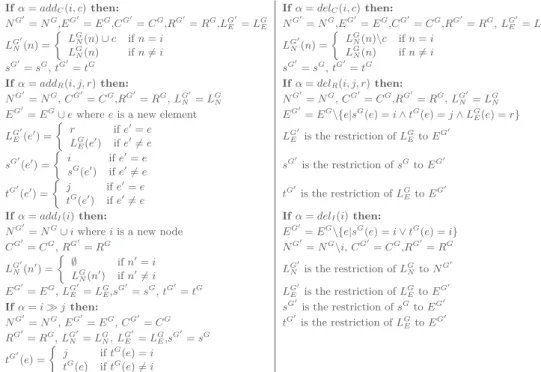
The result of performing the elementary action α on a graph G = (NG, EG, CG, RG,
LG
N, LGE, sG, tG), written G[α], produces the graph G′= (NG
′ , EG′ , CG′ , RG′ , LG′ N, LG ′ E, sG ′ , tG′
) as defined in Figure 3. An action, say α, is a sequence of elementary actions of the form α = a1; a2; . . . ; an. The result of performing α on a graph G is written
Ifα= addC(i, c) then: Ifα= delC(i, c) then: NG′ = NG,EG′ = EG,CG′ = CG,RG′ = RG,LG′ E = LGE NG ′ = NG,EG′ = EG,CG′ = CG,RG′ = RG, LG′ E = LGE LG′ N(n) = ; LG N(n) ∪ c if n = i LG N(n) if n Ó= i LG′ N(n) = ; LG N(n)\c if n = i LG N(n) if n Ó= i sG′ = sG, tG′ = tG sG′ = sG, tG′ = tG
Ifα= addR(i, j, r) then: Ifα= delR(i, j, r) then:
NG′ = NG, CG′ = CG,RG′ = RG, LG′ N = LGN NG ′ = NG, CG′ = CG,RG′ = RG, LG′ N = LGN EG′
= EG∪ e where e is a new element EG′
= EG\{e|sG(e) = i ∧ tG(e) = j ∧ LG E(e) = r} LG′ E(e′) = ; r if e′= e LG E(e′) if e′Ó= e LG′ E is the restriction of LGEto EG ′ sG′ (e′) = ; i if e′= e sG(e′) if e′Ó= e s G′ is the restriction of sGto EG′ tG′ (e′) = ; j if e′= e tG(e′) if e′Ó= e t G′ is the restriction of LG Eto EG ′
Ifα= addI(i) then: Ifα= delI(i) then:
NG′
= NG∪ i where i is a new node EG′
= EG\{e|sG(e) = i ∨ tG(e) = i}
CG′ = CG, RG′ = RG NG′ = NG\i, CG′ = CG,RG′ = RG LG′ N(n′) = ; ∅ if n′= i LG N(n′) if n′Ó= i LG′ N is the restriction of LGNto NG ′ EG′ = EG, LG′ E = LGE,sG ′ = sG, tG′ = tG LG′ E is the restriction of LGEto EG ′ Ifα= i ≫ j then: sG′ is the restriction of sGto EG′ NG′ = NG, EG′ = EG, CG′ = CG tG′ is the restriction of LG Eto EG ′ RG′ = RG, LG′ N = LGN, LG ′ E = LGE,sG ′ = sG tG′ (e) = ; j if tG(e) = i tG(e) if tG(e) Ó= i
Figure 3 Summary of the effects of elementary actions.
◮Definition 9 (Rule, LDRS). A rule ρ is a pair (lhs,α) where lhs, called the left-hand side,
is an attributed graph with C2PDL formulae as attributes and α, called the right-hand side, is an action. Rules are usually written lhs → α. A logically decorated rewriting system, LDRS, is a set of rules.
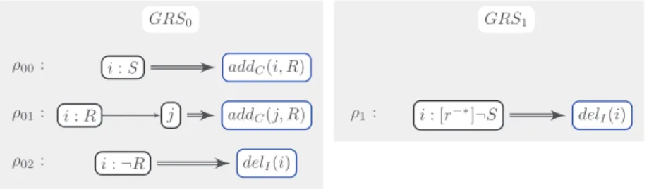
It is noteworthy that the left-hand side of a rule is an attributed graph, that is it can contain nodes labeled with C2PDL formulae. This is not insignificant. Indeed, these formulae can express reachability expression (closure of a program), non-local properties (universal program), ... These node labelings allow to write more concise and simpler rewriting systems. For instance, Figure 4 provides two LDRSs, GRS0 and GRS1 which remove unreachable nodes from a start state (labeled by S) of an automaton. Without the closure constructor (∗), one would tag that the start states are reachable (label R) (rule ρ00), then say that every neighbor of a reachable node is reachable (rule ρ01) and finally that all nodes that have not been reached by applying the first two rules as much as possible are to be removed (rule
ρ02). GRS0requires the explicit computation of the reachability making the algorithm more complex. On the other hand, GRS1 only uses one rule which says that all nodes that are not reachable from a start state are to be removed (rule ρ1).
It is worth noting that the impact of C2PDL formulae in node labels is not limited to graph rewriting. Indeed, let us consider the term rewriting system of integer arithmetic with multiplication. The classical way to deal with 0s in such a case is to have rules saying that 0 × x 0 and x × 0 0. Considering terms as trees, and thus as graphs, it is also possible to improve on this set of rules by using, for instance, the rule i : × ∧ é((L ∪ R); ×?)∗ê0 i : 0. This rule states that if a node i is such that i : × ∧ é((L ∪ R); ×?)∗ê0, that is to say, node i is labeled by the multiplication operator (i : ×) and there is a path of left- or right-operands (L ∪ R), crossing nodes labeled by the multiplication operator (×?), that leads to a node labeled by 0 (i : é((L ∪ R); ×?)∗ê0), then node i could be labeled by 0 (i : 0).
GRS0 GRS1 i: S addC(i, R) i: R j addC(j, R) i: ¬R delI(i) i: [r−∗]¬S del I(i) ρ00: ρ01: ρ02: ρ1:
Figure 4 Two LDRS dealing with the suppression of unreachable nodes. Rules with atomic
formulae are on the left. The rule with a non-atomic formula is on the right.
i: A j: B k:< β∗> C add
R(j, k, γ); delR(j, k, β)
Figure 5 An example of LDRS. The dashed line represents the program (label) α and the plain
line the program β. The first edge labeled β after an access α on a path toward a C gets a new tag γ.
In Figure 5, we provide an additional toy example which is used later. It consists of one rule which relabels the edge going from node j to k with label (program) γ whenever node
khas access to “information” C. This rule may have different interpretations such as the
modification of access policy to information tagged C.
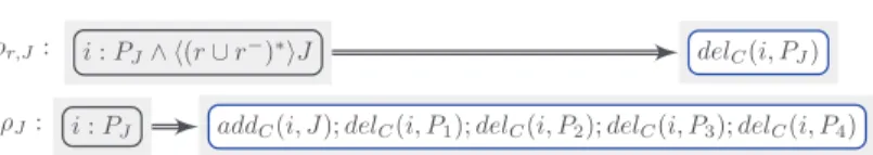
◮Example 10. Back to our running example, we provide a very simple graph rewriting
system R that tries to produce a full and correct grid. It contains 16 rules, that are summarized in Figure 6. The rules ρr,J make sure that when a line (resp. a column or a
square) contains a cell with value J, PJ is no longer available for all the cells on the line
(resp. column or square). The rules ρJ are used to pick one choice among those that are
available.
◮Definition 11 (Match). A match h between a left-hand side lhs and a graph G is a pair
of functions h = (hN, hE), with hN : Nlhs → NG and hE : Elhs→ EG such that:
1. ∀n ∈ Nlhs,∀c ∈ LNlhs(n), hN(n) |= c 2. ∀e ∈ Elhs, LElhs(e) = LEG(hE(e))
3. ∀e ∈ Elhs, sG(hE(e)) = hN(slhs(e)) 4. ∀e ∈ Elhs, tG(hE(e)) = hN(tlhs(e))
The third and the fourth conditions are classical and say that the source and target functions and the match have to agree. The first condition says that for every node n of the left-hand side, the node to which it is associated, h(n), in G has to satisfy every concept that n satisfies. This condition clearly expresses additional negative and positive conditions which are added to the “structural” pattern matching. The second one ensures that the match respects edge labeling.
◮Definition 12 (Rule Application). A graph G rewrites to graph G′ using a rule ρ = (lhs, α)
iff there exists a match h from lhs to G. G′ is obtained from G by performing actions in
h(α)2. Formally, G′= G[h(α)]. We write G →
ρ G′ or G →ρ,hG′.
Confluence of graph rewriting systems is not easy to establish. For instance, orthogonal graph rewrite systems are not always confluent, see e.g.,[7]. That is why we use a notion rewrite strategies to control the use of possible rules. Informally, a strategy specifies the
2
i: PJ∧ é(r ∪ r−)∗êJ delC(i, PJ)
i: PJ addC(i, J); delC(i, P1); delC(i, P2); delC(i, P3); delC(i, P4)
ρr,J:
ρJ:
Figure 6 A summary of the rules of R. In ρr,J, r must be replaced by either R, C or SQ and J
by 1, 2, 3 or 4. In ρJ, J must be replaced by 1, 2, 3 or 4. G→ρG′ G⇒ρG′ (Rule) G⇒s0G ′′ G′′ ⇒s1G′ G⇒s0;s1G′ (Strategy composition) G⇒s0G′ G⇒s0⊕s1G′ (Choice left) G⇒s1G′ G⇒s0⊕s1G′ (Choice right) ¬App(s, G) G⇒s∗G (Closure false) G⇒sG′′ G′′⇒s∗ G′ App(s, G) G⇒s∗G′ (Closure true)
Figure 7 Strategy application rules.
application order of different rules. It does not point to where the matches are to be found nor does it ensure the unicity of the reduction outcome.
◮Definition 13 (Strategy). Given a graph rewriting system R, a strategy is a non-empty
word of the following language defined by s:
s:= ρ (Rule) s; s (Composition) s⊕ s (Choice) s∗ (Closure)
where ρ is any rule in R.
We write G ⇒S G′ when G rewrites to G′ following the rules given by the strategy S.
Informally, the strategy ”ρ1; ρ2” means that rule ρ1 should be applied first, followed by the application of rule ρ2. The strategy ”ρ∗0; (ρ1⊕ ρ2)” means that rule ρ0is applied as far as possible, then followed either by ρ1or ρ2. It is worth noting that the closure is the standard “while” construct: if the strategy we use is s∗, the strategy s is used as long as it is possible
and not an undefined number of times.
◮ Example 14. For the Sudoku example, a possible strategy S1 could be: “As long as
one can eliminate possibilities, do it. Then, when it is no longer the case, make a choice in one of the blank cells and go back to the first step”. S1 may be defined as S1 = (m
r∈{R,C,SQ},J∈[1,4]ρr,J)∗; ((mJ∈[1,4]ρJ); (mr∈{R,C,SQ},J∈[1,4]ρr,J)∗)∗.
In Figure 7, we provide the rules that specify how strategies are used to rewrite a graph. For that, we use the predicate App(s, G) which holds whenever graph G can be rewritten by the strategy s. It is defined as follows:
App(ρ, G) = true iff there exists a match h from the left-hand side of ρ to G
App(s0⊕ s1, G) = App(s0, G) ∨ App(s1, G)
App(s∗
0, G) = true
App(s0; s1, G) = App(s0, G)
It is worth noting that App(s, G) is not meant to denote that the whole strategy can be applied to G, just that the next step can be applied. Indeed, let’s assume the strategy
s= s0; s1 where s0 can be applied but may lead to a state where s1 cannot. In this case
wp(addC(i, c), Q) = Q[addC(i, c)] wp(delC(i, c), Q) = Q[delC(i, c)]
wp(addR(i, j, r), Q) = Q[addR(i, j, r)] wp(delR(i, j, r), Q) = Q[delR(i, j, r)]
wp(addI(i), Q) = Q[addI(i)] • wp(delI(i), Q) = Q[delI(i)]
wp(i >> j, Q) = Q[i >> j] wp(ǫ, Q) = Q
wp(a; α, Q) = wp(a, wp(α, Q))
Figure 8 Weakest pre-conditions for actions.
wp(s0; s1, Q) = wp(s0, wp(s1, Q)) wp(s0⊕ s1, Q) = wp(s0, Q) ∧ wp(s1, Q)
wp(s∗, Q) = inv
s wp(ρ, Q) = App(tag(ρ)) ⇒ wp(tag(αρ), Q)
Figure 9 Weakest pre-conditions for strategies.
4
Proving Correctness of LDRS’s
Equational reasoning and structural induction method represent the main core of proof techniques dedicated to reason about term rewrite systems. Unfortunately, graph rewrite systems do not benefit yet from such established techniques. For example, generalization of equational reasoning to graph rewriting systems is not complete [6]. In this section, we propose a way to specify properties of LDRSs for which we establish a decidable proof procedure.
◮Definition 15 (Specification). A specification SP is a tuple (P re, P ost, R, S) where P re
and P ost are C2PDL formulas, R is a graph rewriting system and S is a strategy.
A specification SP is said to be correct iff for all graphs G, G′ such that G ⇒S G′ and
G|= P re, then G′|= P ost.
In order to show the correctness of a specification, we follow a Hoare-calculus style and compute the weakest condition wp(S, P ost). For that, we define the weakest pre-conditions of a formula P ost induced by a strategy, a rule, an action and an elementary action. They are presented in Figure 8 for the elementary actions and Figure 9 for strategies. The weakest pre-condition of an elementary action, say a, and a post-condition Q is defined as wp(a, Q) = Q[a] where Q[a] stands for the pre-condition consisting of Q to which is applied a substitution induced by the action a that we denote by [a]. The notion of substitution used here is the one of Hoare-calculi [11].
◮Definition 16 (Substitutions). To each elementary action a is associated a substitution,
written [a], such that for any graph G, (G |= φ[a]) ⇔ (G[a] |= φ).
It is worth noting that substitutions are, in all generality, not defined as formulae of C2PDL. They are defined as a new constructor whose meaning is that the weakest pre-conditions as defined above are correct. There is no reason whatsoever to think that the addition of a constructor for substitutions is harmless, in general. It is a very interesting problem to figure out for which logics they can be introduced as it is a strong indication that such a logic may be suitable to study the correction of programs. It is one of the central results of [5] that C2PDL is closed under substitutions allowing us to use them freely in the following.
i: {ia, PJ} addC(ia, J ); delC(ia, P1); delC(ia, P2); delC(ia, P3); delC(ia, P4)
tag(ρJ) :
Figure 10 The rule ρJ is modified into tag(ρJ) with tag(i) = ia.
Apart from wp(ρ, Q), the weakest pre-conditions defined in here are the usual ones. As in any other framework using Hoare logic, it requires the definition of an invariant(inv) for each loop that has to be provided by the user.
The weakest pre-condition of a rule ρ = (lhsρ, αρ) and a post-condition Q is given by
wp(ρ, Q) = App(tag(ρ)) ⇒ wp(tag(αρ), Q) where tag : Nlhsρ → Σ is a function which
associates to every node, n, of the left-hand side of rule ρ, a fresh name in Σ. These new names are used to keep track of the matching locations within potential graphs rewritten by different instances of ρ during the execution of a strategy. tag(ρ) = (tag(lhsρ), tag(αρ))
where tag(lhsρ) is a named graph which consists of the graph lhsρ where the node labeling
function is augmented by tag, i.e., for all nodes, n, of lhsρ, LNtag(lhsρ)(n) = LNlhsρ(n)∪tag(n).
tag(αρ) is obtained from αρ by substituting every node (in Nlhsρ), say i, by tag(i). Figure 10
gives an example turning the left-hand side of a rule into a named graph via a function tag. The formula App(tag(ρ)) expresses the applicability of the rule tag(ρ). In other words, it expresses the existence of a match of the left-hand side of tag(ρ). More precisely App(tag(ρ)) is defined as follows:
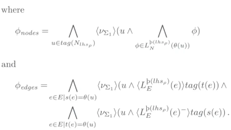
App(tag(ρ)) = φnodes∧ φedges
where φnodes= Þ u∈tag(Nlhsρ) éνΣ1ê(u ∧ Þ φ∈Lþ(lhsρ)N (θ(u)) φ) and φedges= Þ e∈E|s(e)=θ(u) éνΣ1ê(u ∧ éL þ(lhsρ) E (e)êtag(t(e)) ∧ Þ e∈E|t(e)=θ(u) éνΣ1ê(u ∧ éL þ(lhsρ) E (e) −êtag(s(e)) .
φnodes states that the first condition of Definition 11 is satisfied i.e., all formulae satisfied
by a node of the left-hand side have to be satisfied by its image in the graph. φedges does
the same with edges: the label of the corresponding edges are the same and the source and target functions fulfill the matching compatibly condition.
Tagging a rule may seem to reduce its applicability. Indeed, by choosing a new name for each node of the left-hand side, the rule can now be applied only at the nodes of the graph named accordingly. Let ρ be a rule such that LHSρ= (Nρ= {i0, . . . in}, Eρ,Cρ,Rρ, LNρ, LEρ,
sρ, tρ) is its left-hand side. In order to prove that the application of ρ on a graph
G= (NG, EG,CG,RG, LNG, LEG, sG, tG) is correct, one has to verify that for every match
h= (hN, hE) (as defined in Definition 11), the post-condition is satisfied after the
transform-ation associated with ρ is applied at the hN(ik)’s. Instead of showing that, the verification
procedure proves that for any graph, if the rule can be applied at the θ(u)’s, where θ is the function that associates to each name of Σ a node of G and u ∈ tag(ρ), the post-condition is satisfied after performing the transformation. As the u’s are fresh names, they do not have any impact on the previous characterization of the graphs. Thus, the validity of
vc(ρ, Q) = ⊤ vc(s0; s1, Q) = vc(s0, wp(s1, Q)) ∧ vc(s1, Q)
vc(s0⊕ s1, Q) = vc(s0, Q) ∧ vc(s1, Q)
vc(s∗, Q) = (inv
s∧ NApp(s) ⇒ Q) ∧ (invs⇒ wp(s, invs)) ∧ vc(s, invs)
Figure 11 Verification conditions.
wp(ρ, P ost) actually states that whatever the choice of θ is, if the rule can be applied, then the post-condition will be satisfied after it is fired.
The weakest pre-condition associated to the closure of a strategy, say s∗, and a post-condition Q is defined as wp(s∗, Q) = inv
s where invs is an invariant (C2PDL formula)
associated to the strategy s. Roughly speaking s∗ could be seen as a while-loop which needs invariants associated with additional proof obligations defined by means of the function vc (verification conditions) given in Figure 11.
Informally, the predicate NApp(s), used in the definition of vc, the verification conditions function, says that the strategy s cannot be applied. To express NApp(s), one may wonder whether it is possible to use the negation of App(s). The answer is negative since App has been defined using dedicated names, that is to say a rule is applied at a specific place defined by the added names introduced by the function tag. Intuitively, if one wants to express that there is no match for a rule whose left-hand side contains a cycle (e.g., the second graph of Figure 12), then universal quantification is required. For instance, in that case it would be ∀i, j.[νΣ1](i ⇒ [R](j ⇒ [R]¬i)). One of them can be discarded to produce the expression ∀i.[νΣ1](i ⇒ [R][R]¬i). Alas, this cannot be expressed in C2PDL. The names only allow to express existential quantifiers. Indeed, to express universal quantifiers, one needs to extend the logic with the binder ↓ of hybrid logic which is enough to make the logic undecidable[2].
To express formally NApp(s) in C2PDL, one needs to introduce some additional definitions first.
◮Definition 17 (Explicitly Named Nodes, Non-Oriented Cycles). An explicitly named node is
a node such that each disjunct of the disjunctive normal form of its label contains a name. A non-oriented cycle, c, is a finite list of nodes c = [n0, . . . , nk] such that (i) nk = n0 and (ii) ∀κ ∈ [0, k − 1], ∃r ∈ Π0 such that (nκ, nκ+1) ∈ R(r) or (nκ+1, nκ) ∈ R(r).
◮ Definition 18 (Grove and Thicket). A grove is a disjoint union of thickets. A thicket
is a connected graph such that it does not contain any non-oriented cycle composed only of non explicitely named nodes. We call a strategy S relative to a rewriting system R a
grove-strategy if the left-hand sides of all the rules appearing under a closure are groves.
Let lhs be a left-hand side. Let us split Nlhs into TE, the set of explicitly named nodes,
and TI = Nlhs\TE. For each maximally connected subgraph composed only of nodes in TI,
a distinguished node ri is selected. If there is a maximally connected subgraph composed
only of explicitly named nodes, an ri is also picked for it. Now, everything is ready to define
NApp( s). 1. NApp(ρ) =x ri[νΣ1]NA(ri,∅) 2. NA(n, V ) = (x φ∈LN(n)¬φ) ∨ ( x e∈E|s(e)=n|s(e)∈TE∪(TI\V )[LE(e)]NA(t(e), V ∪ {n})) ∨ (x e∈E|t(e)=n|t(e)∈TE∪(TI\V )[LE(e) −]NA(s(e), V ∪ {n})) if n Ó∈ V 3. NA(n, V ) = ¬µ(n) if n ∈ TE∩ V
4. NApp(s0⊕ s1) = NApp(s0) ∧ NApp(s1)
5. NApp(s∗) = f alse
A B A B A
Figure 12 These two graphs are indistinguishable without names.
Rule 2 is the most involved. NA(n, V ) is used to describe what has to be true for a node different from n. V is used to track which nodes have already been visited. xφ∈LN(n)¬φ states that there is at least one of the formulae satisfied by n that is not satisfied while x
e∈E|s(e)=n|s(e)∈TE∪(TI\V )[LE(e)]NA(t(e), V ∪ {n}) means that there is a neighbor of n using
an outgoing edge that cannot find a match. xe∈E|t(e)=n|t(e)∈TE∪(TI\V )[LE(e)−]NA(s(e), V ∪
{n}) has the same signification but for incoming edges. Rule 3 is used to recall the names of the explicitly named nodes that have already been visited without creating a cycle in the execution. Rules 4 to 6 are exactly the negation of App(s, G). Rule 1 says that for at least one ri, it is not possible to find a node that would be a match. It is noteworthy that there is
no rule for N ∈ TI∩ V since the considered left-hand side has to be a grove.
◮Example 19. The rules of the Sudoku example are simple, having only one-node left-hand
side, and thus not very interesting as far as NApp is concerned. We will thus consider the rule, say ρ, of Figure 5. There is only one connected subgraph so one has to pick one distinguished node r0. Let us choose, randomly, the node j as r0. Then NApp(ρ) = [νΣ1]NA(j, ∅). As j is not explicitly named, NA(j, ∅) = ¬B ∨ [β]NA(k, {j}) ∨ [α−]NA(i, {j}). As i is not explicitly named either, NA(i, {j}) = ¬A as the only neighbor of i is j. Finally, NA(k, {j}) = [β∗]¬C as the only neighbor of k is j. Thus NApp(ρ) = [νΣ1](¬B ∨ [β][β
∗]¬C ∨ [α−]¬A).
Given a specification SP , the correctness of SP amounts to verify the validity of the formula CorrSP = vc(S, post) ∧ (pre ⇒ wp(S, post)). It can be shown that CorrSP is a
C2PDL formula due to the closure by substitutions of C2PDL [5]. Therefore we can state the soundness of our calculus in the following theorem.
◮ Theorem 20. Let SP = (P re, P ost, R, S) be a specification where P re and P ost are
C2PDL formulas, S is a grove-strategy relative to LDRS R. If the formula CorrSP =
vc(S, post) ∧ (pre ⇒ wp(S, post)) is valid then for all graphs G and G′, if G ⇒
S G′, then
G|= pre implies G′|= post.
CorrSP being a formula of C2PDL, one gets the following corollary from theorem 7. ◮ Corollary 21. Let SP = (P re, P ost, R, S) be a specification where P re and P ost
are C2PDL formulas, S is a grove-strategy relative to LDRS R. The verification of the correctness of SP is decidable.
◮ Example 22. The example of Figure 13 contains one rule that is applied as long as
possible. As the closure is used, an invariant has to be specified. We choose éνΣ1êx which is obviously an invariant of the loop. The specifications differ on the post-condition, the first one being what we would expect, that is all elements are labelled A, and the other one being the exact opposite. Both specifications are deemed partially correct. Indeed, as
wp(ρ∗
1, P ost) = inv = éνΣ1êx, P re ⇒ wp(ρ ∗
1, P ost) = ⊤. Furthermore, as vc(ρ∗1, P ost) = (inv∧App(ρ1) ⇒ inv[addC(i, A)])∧(inv∧NApp(ρ1) ⇒ P ost)∧vc(ρ1, inv) and vc(ρ1, inv) = ⊤ and inv ⇒ inv = ⊤, vc(ρ∗
1, P ost) = inv ∧ NApp(ρ1) ⇒ P ost). But then, as NApp(ρ1) = [νΣ1]⊥, inv ∧ NApp(ρ1) = ⊥ and thus vc(ρ
∗
1, P ost) = ⊤ independently of the post-condition. The fact that two specifications leading to opposite results would be both considered correct
i addC(i, A) ρ1: SP10= (éνΣ1ê(x ∧ ¬A), [νΣ1]A, {ρ1}, ρ ∗ 1) SP11= (éνΣ1ê(x ∧ ¬A), éνΣ1ê¬A, {ρ1}, ρ ∗ 1)
Figure 13 Scholastic examples of specification. Both of the specifications are partially correct.
seems to be an error but the fact is that the program will never stop and, actually, no result is ever reached.
It is noteworthy that the choice of the invariant is, as usual in Hoare logic [11], far from innocent. Let’s assume we chose inv = ⊤ instead. Then, the only difference is that now
inv∧ NApp(ρ1) = NApp(ρ1) = [νΣ1]⊥. But then, inv ∧ NApp(ρ1) ⇒ [νΣ1]¬A is true but not inv ∧ NApp(ρ1) ⇒ éνΣ1êA. A poor choice of inv can prevent someone from proving a program correct.
The example of the Sudoku can be proven to be valid with a suitable choice of P re, P ost and inv.
5
Related work
One of the main features of the class of rewriting systems we introduce in this paper consists in specifying application conditions as logic formulas that label nodes of the left-hand sides. This is, to our knowledge, a new approach to specify application conditions. In [9] the idea of additional (negative) application conditions has been introduced in a framework based on category theory.
Our second contribution is to introduce a decidable verification procedure for the con-sidered rewrite systems and the logic used to express system properties. The problem of reasoning about graph transformations is known to be complex in its full generality [12].
One approach to program verification, as exemplified by [10, 16], is similar to the one we pursue here, i.e., the goal is to generate the weakest pre-condition for a condition to be satisfied. Our method strongly diverges from theirs in very key points, though. First and foremost, their rewriting systems are based on algebraic methods whereas ours are purely algorithmic. Secondly, our graphs are logically attributed, that is each node is labeled with formulas. Another difference lies in the considered logics. Indeed, the logic presented in [16] is equivalent to monadic second-order logic. It thus allows to express second-order quantification which is out of the scope of our logic. The one in [10] is equivalent to first-order graph formulas whose expressivity is not comparable to ours (i.e., there are formulas that can be expressed in one logic but not in the other and vice versa). Both monadic second-order and first-order graph logics are undecidable. On the other hand, we have carefuly chosen an extension of dynamic logic that preserves decidability. Last but not least, the way they compute the pre-conditions is also much different from ours. We use the notion of substitutions whereas their conditions are built incrementally on the rules.
In [13], the authors also use a stronger logic, monadic second-order logic again, and the verification problem is decidable. This is due to the fact that their transformations are bisimulation-generic whereas ours are not. Furthermore they do not label nodes. In both cases, the core of the reflexion is centered in modifications of the structure of the data (that is how general classes of nodes and edges interact). On the other hand, we are able to do the
core of these transformation but our focus is on localized modifications that is a change at the instance level.
Another approach to the verification of graph transformation is the classical model-checking applied in the case where states are specified by graphs [17]. This approach, which needs the development of a possibly infinite transition systems, departs from ours.
A verification method of graph transformation is tackled in [14] where a set of forbidden graphs is given and where context-free graph grammars are used instead of logics to define post-conditions. This method is quite different from ours.
In [3], a logic dedicated to mimic graph transformations has been introduced. That logic can also be used to specify properties over graph transformations. The expressive power of that logic is very rich but its validity problem is not decidable.
In [6], an extension of equational logic to graph transformation has been investigated. Theories generated by such logic are not recursively enumerable in general. Thus no completeness nor decidability results can be expected. In addition, in the considered logic bisimilar graphs cannot be distinguished.
The modification of Knowledge Bases is a much different but very active field. Belief revision [1] deals with the addition of new knowledge and how to modify the Knowledge Base so that it is still consistent. That means that a lot of modifications may be hidden in one update action. This is quite a different approach as we want, on the other hand, to know exactly what actions are performed and use that to define our new knowledge.
The work in [4] is heading toward the same goal as the present paper but both the programming language, that is slightly less expressive and imperative, and the considered logic are different.
6
Conclusion
We have presented a new class of graph rewrite systems, LDRSs, where left-hand sides can express additional application conditions defined as C2PDL formulas. We defined computations with these systems by means of rewrite strategies. There is certainly much work to be done around such systems with logically decorated left-hand sides. For instance, the extension to narrowing derivations, which is a matter of future work, would use an involved unification algorithm taking into account the underlying logic. We have also presented a sound Hoare-like calculus for specifications with pre- and post-conditions in C2PDL and show that the considered correctness problem is decidable. These positive achievements deserve to be extended to other logics which we intend to investigate in the future.
References
1 Carlos E. Alchourrón, Peter Gärdenfors, and David Makinson. On the logic of theory change: Partial meet contraction and revision functions. J. Symb. Log., 50(2):510–530, 1985. doi:10.2307/2274239.
2 Carlos Areces and Balder ten Cate. Hybrid logics. In Studies in Logic and Practical
Reasoning, volume 3, pages 821–868. Elsevier, 2007.
3 Philippe Balbiani, Rachid Echahed, and Andreas Herzig. A dynamic logic for termgraph rewriting. In 5th International Conference on Graph Transformations (ICGT), volume 6372 of Lecture Notes in Computer Science, pages 59–74. Springer, 2010.
4 Jon Haël Brenas, Rachid Echahed, and Martin Strecker. A Hoare-like calculus using the SROIQ σ logic on transformations of graphs. In Theoretical Computer Science – 8th IFIP
TC 1/WG 2.2 International Conference, TCS 2014, Rome, Italy, September 1-3, 2014. Proceedings, pages 164–178, 2014. doi:10.1007/978-3-662-44602-7_14.
5 Jon Hael Brenas, Rachid Echahed, and Martin Strecker. C2PDLS: A combination of
combinatory and converse PDL with substitutions. 2015. URL: http://lig-membres. imag.fr/echahed/c2pdls.pdf.
6 Ricardo Caferra, Rachid Echahed, and Nicolas Peltier. A term-graph clausal logic:
Com-pleteness and incomCom-pleteness results. Journal of Applied Non-classical Logics, 18(4):373– 411, 2008.
7 Rachid Echahed. Inductively sequential term-graph rewrite systems. In 4th International Conference on Graph Transformations, ICGT, volume 5214 of Lecture Notes in Computer Science, pages 84–98. Springer, 2008.
8 Michael J. Fischer and Richard E. Ladner. Propositional dynamic logic of regular programs. J. Comput. Syst. Sci., 18(2):194–211, 1979. doi:10.1016/0022-0000(79)90046-1. 9 Annegret Habel, Reiko Heckel, and Gabriele Taentzer. Graph grammars with
negat-ive application conditions. Fundam. Inform., 26(3/4):287–313, 1996. doi:10.3233/ FI-1996-263404.
10 Annegret Habel and Karl-Heinz Pennemann. Correctness of high-level transformation sys-tems relative to nested conditions. MSCS, 19:245–296, 2009.
11 C. A. R. Hoare. An axiomatic basis for computer programming. Commun. ACM,
12(10):576–580, 1969. doi:10.1145/363235.363259.
12 Neil Immerman, Alex Rabinovich, Tom Reps, Mooly Sagiv, and Greta Yorsh. The boundary
between decidability and undecidability for transitive-closure logics. In Jerzy Marcinkowski and Andrzej Tarlecki, editors, Computer Science Logic, volume 3210 of Lecture Notes in
Computer Science, pages 160–174. Springer Berlin / Heidelberg, 2004. URL: http://www.
cs.umass.edu/~immerman/pub/cslPaper.pdf.
13 Kazuhiro Inaba, Soichiro Hidaka, Zhenjiang Hu, Hiroyuki Kato, and Keisuke Nakano. Graph-transformation verification using monadic second-order logic. In Proceedings of
the 13th International ACM SIGPLAN Conference on Principles and Practice of De-clarative Programming, July 20-22, 2011, Odense, Denmark, pages 17–28, 2011. doi:
10.1145/2003476.2003482.
14 Barbara König and Javier Esparza. Verification of graph transformation systems with context-free specifications. In Graph Transformations – 5th International Conference,
ICGT 2010, Enschede, The Netherlands, September 27 – October 2, 2010. Proceedings,
pages 107–122, 2010. doi:10.1007/978-3-642-15928-2_8.
15 Solomon Passy and Tinko Tinchev. An essay in combinatory dynamic logic. Inf. Comput., 93(2):263–332, 1991. doi:10.1016/0890-5401(91)90026-X.
16 Christopher M. Poskitt and Detlef Plump. Verifying monadic second-order properties of graph programs. In Graph Transformation – 7th International Conference, ICGT 2014,
Held as Part of STAF 2014, York, UK, July 22-24, 2014. Proceedings, pages 33–48, 2014.
doi:10.1007/978-3-319-09108-2_3.
17 Arend Rensink, Ákos Schmidt, and Dániel Varró. Model checking graph transformations: A comparison of two approaches. In Graph Transformations, Second International Conference,
ICGT 2004, Rome, Italy, September 28 – October 2, 2004, Proceedings, pages 226–241, 2004.
doi:10.1007/978-3-540-30203-2_17.
18 Grzegorz Rozenberg, editor. Handbook of Graph Grammars and Computing by Graph Transformations, Volume 1: Foundations. World Scientific, 1997.