To link to this article : DOI :
10.1007/s10462-016-9532-4
URL : https://doi.org/10.1007/s10462-016-9532-4
To cite this version :
Ionescu, Radu Tudor and Ionescu, Andreea Lavinia and
Mothe, Josiane and Popescu, Dan Patch Autocorrelation Features: A
translation and rotation invariant approach for image classification. (2016)
Artificial Intelligence Review, 2016. pp. 1-32. ISSN 0269-2821
O
pen
A
rchive
T
OULOUSE
A
rchive
O
uverte (
OATAO
)
OATAO is an open access repository that collects the work of Toulouse researchers and
makes it freely available over the web where possible.
This is an author-deposited version published in :
http://oatao.univ-toulouse.fr/
Eprints ID : 18821
Any correspondence concerning this service should be sent to the repository
administrator: [email protected]
Patch Autocorrelation Features: A translation and
rotation invariant approach for image classification
Radu Tudor Ionescu · Andreea LaviniaIonescu · Josiane Mothe · Dan Popescu
Abstract The autocorrelation is often used in signal processing as a tool for find-ing repeatfind-ing patterns in a signal. In image processfind-ing, there are various image analysis techniques that use the autocorrelation of an image in a broad range of applications from texture analysis to grain density estimation. This paper provides an extensive review of two recently introduced and related frameworks for image representation based on autocorrelation, namely Patch Autocorrelation Features (PAF) and Translation and Rotation Invariant Patch Autocorrelation Features (TRIPAF). The PAF approach stores a set of features obtained by comparing pairs of patches from an image. More precisely, each feature is the euclidean dis-tance between a particular pair of patches. The proposed approach is successfully evaluated in a series of handwritten digit recognition experiments on the popular MNIST data set. However, the PAF approach has limited applications, because it is not invariant to affine transformations. More recently, the PAF approach was extended to become invariant to image transformations, including (but not limited to) translation and rotation changes. In the TRIPAF framework, several features are extracted from each image patch. Based on these features, a vector of similar-ity values is computed between each pair of patches. Then, the similarsimilar-ity vectors are clustered together such that the spatial offset between the patches of each pair is roughly the same. Finally, the mean and the standard deviation of each similarity value are computed for each group of similarity vectors. These statis-tics are concatenated to obtain the TRIPAF feature vector. The TRIPAF vector essentially records information about the repeating patterns within an image at various spatial offsets. After presenting the two approaches, several optical char-R. T. Ionescu
University of Bucharest, 14 Academiei, Bucharest, Romania, E-mail: [email protected]
A. L. Ionescu, D. Popescu
Politehnica University of Bucharest, 313 Splaiul Independentei Street, Bucharest, Romania, E-mail: [email protected], dan popescu [email protected]
J. Mothe ´
Ecole Sup´erieure du Professorat et de l’ ´Education, Universit´e de Toulouse, IRIT, UMR 55005 CNRS, 118, Route de Narbonne, Toulouse, France, E-mail: [email protected]
acter recognition and texture classification experiments are conducted to evaluate the two approaches. Results are reported on the MNIST (98.93%), the Brodatz (96.51%), and the UIUCTex (98.31%) data sets. Both PAF and TRIPAF are fast to compute and produce compact representations in practice, while reaching ac-curacy levels similar to other state-of-the-art methods.
Keywords image autocorrelation · patch-based method · optical character recognition · texture classification · rotation invariant method · translation invariant method · MNIST · Brodatz · UIUCTex
1 Introduction
Artificial intelligence is a vast domain with important applications in many fields (Valipour et al, 2013; Valipour, 2015a,b; Laalaoui and Bouguila, 2015; Ionescu et al, 2016), including computer vision (Szeliski, 2010; Ionescu and Popescu, 2016). The classical problem in computer vision is that of determining whether or not the image data contains some specific object, feature, or activity. Object recogni-tion, face recognirecogni-tion, texture classification and optical character recognition are particular formulations of this problem, the last two of them being approached in the current work. Optical character recognition is widely employed as a form of acquiring digital information from printed paper documents such as passport documents, business cards, or even historical documents, so that they can be elec-tronically stored, edited or searched. On the other hand, texture classification is extremely useful in industrial and biomedical surface inspection, for example for defects or disease identification. Texture classification is also employed for ground classification and segmentation of satellite or aerial imagery. Hence, there are many potential applications of the two frameworks presented in this work.
Computer vision researchers have developed sophisticated methods for various image classification tasks. Virtual SVM (DeCoste and Sch¨olkopf, 2002), boosted stumps (K´egl and Busa-Fekete, 2009), convolutional neural networks (LeCun et al, 1998; Ciresan et al, 2012) or deep Boltzmann machines (Salakhutdinov and Hin-ton, 2009) are sophisticated state-of-the-art learning frameworks used for optical character recognition. However, simple methods such as the k-Nearest Neighbor (k-NN) model have also obtained very good recognition results, sometimes being much better than more sophisticated techniques. Some of the techniques that fall in this category of simple yet very accurate methods, and worth to be mentioned, are the k-NN models based on Tangent distance (Simard et al, 1996), shape context matching (Belongie et al, 2002), non-linear deformation (Keysers et al, 2007), and Local Patch Dissimilarity (Dinu et al, 2012), respectively. While optical character recognition can successfully be approached with a simple technique, more complex image classification tasks require more sophisticated methods, naturally because the methods have to take into account several aspects such as translation, rotation, and scale variations, illumination changes, viewpoint changes, partial occlusions and noise. Among the rather more elaborate state-of-the-art models used in image classification are bag of visual words (Csurka et al, 2004; Liu et al, 2011; Ionescu et al, 2013), Fisher Vectors (Perronnin and Dance, 2007; Perronnin et al, 2010), and deep learning models (Krizhevsky et al, 2012; Socher et al, 2012; Simonyan and Zisserman, 2014; Szegedy et al, 2015).
in this category of simple yet very accurate methods, and worth to be mentioned,
This paper presents two feature representation for images that are based on the autocorrelation of the image with itself. The first representation is a simple approach in which each feature is determined by the euclidean distance between a pair of patches extracted from the image. To reduce the time necessary to com-pute the feature representation, patches are extracted at a regular interval by using a dense grid over the image. This feature representation, which was initially introduced in (Ionescu et al, 2015a), is termed Patch Autocorrelation Features (PAF). Ionescu et al (2015a) have shown that PAF exibits state-of-the-art perfor-mance in optical character recognition. However, the PAF approach is affected by affine transformations and it requires additional improvements in order to solve1
more complex image classification tasks, such as texture classification, for exam-ple. Ionescu et al (2015b) have proposed an extension of PAF that is invariant to image transformations, such as translation and rotation changes. Naturally, this extension involves more elaborate computations, but the resulted feature vector is actually more compact, since it involves the vector quantization of pairs of patches according to the spatial offset between the patches in each pair. Instead of directly comparing the patches, the extended approach initially extracts a set of features from each patch. The extended feature representation is termed Translation and Rotation Invariant Patch Autocorrelation Features (TRIPAF).
Several handwritten digit recognition experiments are conducted in this work in order to demonstrate the performance gained by using the PAF representa-tion instead of a standard representarepresenta-tion based on raw pixel values (a common approach for optical character recognition). More precisely, experiments are per-formed using two different classifiers (k-NN and SVM) on original and deslanted images from the MNIST data set. Experiments are conducted on only 1000 images, but also on the entire MNIST data set. The empirical results obtained in all the experiments indicate that the PAF representation is constantly better than the standard representation. The best results obtained with the PAF representation are similar to some of the state-of-the-art methods (K´egl and Busa-Fekete, 2009; Salakhutdinov and Hinton, 2009). The advantage of PAF is that it is easy and fast to compute.
A series of texture classification experiments are also conducted in the present work to evaluate the extended version of PAF, namely TRIPAF, in a more difficult setting. Two popular texture classification data sets are used for the evaluation, specifically Brodatz and UIUCTex. The empirical results indicate that TRIPAF can significantly improve the performance over a system that uses the same fea-tures, but extracts them from entire images. By itself, TRIPAF is invariant to rotation and translation changes, and for this reason, it makes sense to combine it with a scale invariant system in order to further improve the performance. As such, the system based on TRIFAF was combined with the bag of visual words (BOVW) framework of Ionescu et al (2014b) through multiple kernel learning (MKL) (Gonen and Alpaydin, 2011). The BOVW framework is based on cluster-ing SIFT descriptors (Lowe, 1999) into visual words, which are scale invariant. The performance level of the combined approach is comparable to the state-of-the-art methods for texture classification (Zhang et al, 2007; Nguyen et al, 2011; Quan et al, 2014).
1 with a reasonable degree of accuracy
This paper presents two feature representation for images that are based on
1
affine transformations and it requires additional improvements in order to solve1
images from the MNIST data set. Experiments are conducted on only 1000 images,
The idea behind the PAF and the TRIPAF approaches is to represent the repeating patterns that occur in the image through a set of features. Thus, they provide a way of representing the image autocorrelation that is useful for learning the repeating patterns in order to classify images. A key difference from previous works using the autocorrelation for texture classification (Horikawa, 2004b,a; Toy-oda and Hasegawa, 2007) is that TRIPAF obtains significantly better performance for this task. Moreover, TRIPAF provides a compact representation that can be computed fast.
To summarize, the contributions of this overview paper are:
• It provides an extensive description of PAF, a simple and efficient feature representation for handwritten digit recognition and simple image classification tasks (Section 3);
• It gives an extensive presentation of TRIPAF, a compact, efficient and invari-ant feature representation for texture classification and more complex image classification task (Section 4);
• It presents classification results obtained with PAF on the MNIST data set (Section 6);
• It presents classification results obtained with TRIPAF on the Brodatz and UIUCTex data sets (Section 7);
• It provides empirical evidence that TRIPAF is invariant to rotation and mirror transformations (Section 7.6).
2 Related Work
2.1 Autocorrelation in Image Analysis
The autocorrelation is a mathematical tool for finding repeating patterns which has a wide applicability in various domains such as signal processing, optics, statistics, image processing, or astrophysics. In signal processing, it is used to find repetitive patterns in a signal over time. Images can also be regarded as spatial signals. Thus, it makes sense to measure the spatial autocorrelation of an image. Certainly, the autocorrelation has already been used in image and video processing (Brochard et al, 2001; Popovici and Thiran, 2001; Horikawa, 2004b; Toyoda and Hasegawa, 2007; Kameyama and Phan, 2013; Yi and Pavlovic, 2013; Haouas et al, 2016). Brochard et al (2001) present a method for feature extraction from texture im-ages. The method is invariant to affine transformations, this being achieved by transforming the autocorrelation function (ACF) and then by determining an in-variant criterion which is the sum of the coefficients of the discrete correlation matrix.
A method for using higher order local autocorrelations (HLAC) of any order as features is presented in (Popovici and Thiran, 2001). The method exploits the special form of the inner products of autocorrelations and the properties of some kernel functions used by SVM. Toyoda and Hasegawa (2007) created large mask patterns for HLAC features and constructed multi-resolution features to support large displacement regions. The method is applied to texture classification and face recognition. However, Toyoda and Hasegawa (2007) apply their method on only 32 Brodatz textures and obtain their best accuracy rate of 83.0% with 19 training samples per class. By contrast, TRIPAF is evaluated on all the 111 repeating patterns that occur in the image through a set of features. Thus, they
Brodatz textures using only 3 training samples per class, a considerably more difficult setting. However, the accuracy of TRIPAF (92.85%) is nearly 10% better. Kernel canonical correlation analysis based on autocorrelation kernels is ap-plied to invariant texture classification in (Horikawa, 2004b). The autocorrelation kernels represent the inner products of the autocorrelation functions of original data. In (Horikawa, 2004a), SVM based on autocorrelation kernels are used for texture classification invariant to similarity transformations and noise. Different from these works (Horikawa, 2004b,a), the TRIPAF framework is evaluated on the entire Brodatz data set, demonstrating good results for more than a few kinds of texture.
Kameyama and Phan (2013) explored the nature of the (Local) Higher-Order Moment kernel of various orders as measures for image similarity. The Higher-Order Moment kernel enables efficient utilization of higher-order autocorrelation features in images. Through sensitivity evaluation and texture classification exper-iments, the authors found that the studied kernel allows to control the selectivity of the similarity evaluation.
Yi and Pavlovic (2013) propose an autocorrelation Cox process that encodes spatio-temporal context in a video. In order to infer the autocorrelation struc-ture relevant for classification, they adopt the information gain feastruc-ture selection principle. The authors obtain state-of-the-art performance on action recognition in video.
Haouas et al (2016) focus on the combination of two important image features, the spectral and the spatial information, for remote sensing image classification. Their results show the effectiveness of introducing the spatial autocorrelation in the pixel-wise classification process.
2.2 Patch-based Techniques
As many other computer vision techniques (Efros and Freeman, 2001; Deselaers et al, 2005; Guo and Dyer, 2007; Barnes et al, 2011; Michaeli and Irani, 2014), the PAF map considers patches rather than pixels, in order to capture distinctive features such as edges, corners, shapes, and so on. In other words, the PAF repre-sentation stores information about repeating edges, corners, and other shapes that can be found in the analyzed image. For numerous computer vision applications, the image can be analyzed at the patch level rather than at the individual pixel level or global level. Patches contain contextual information and have advantages in terms of computation and generalization. For example, patch-based methods produce better results and are much faster than pixel-based methods for texture synthesis (Efros and Freeman, 2001). However, patch-based techniques are still heavy to compute with current machines, as stated in (Barnes et al, 2011). To reduce the time necessary to compute the PAF representation, patches are com-pared using a grid over the image. The density of this grid can be adjusted to obtain the desired trade-off between accuracy and speed.
A paper that describes a patch-based approach for rapid image correlation or template matching is (Guo and Dyer, 2007). By representing a template image with an ensemble of patches, the method is robust with respect to variations such as local appearance variation, partial occlusion, and scale changes. Rectangle Moment kernel of various orders as measures for image similarity. The Higher-Order Moment kernel enables efficient utilization of higher-order autocorrelation
filters are applied to each image patch for fast filtering based on the integral image representation.
An approach to object recognition was proposed by Deselaers et al (2005), where image patches are clustered using the EM algorithm for Gaussian mixture densities and images are represented as histograms of the patches over the (dis-crete) membership to the clusters. Patches are also regarded in (Paredes et al, 2001), where they are classified by a nearest neighbor based voting scheme.
Agarwal and Roth (2002) describe a method where images are represented by binary feature vectors that encode which patches from a codebook appear in the images and what spatial relationship they have. The codebook is obtained by clustering patches from training images whose locations are determined by interest point detectors.
Passino and Izquierdo (2007) propose an image classification system based on a Conditional Random Field model. The model is trained on simple features obtained from a small number of semantically representative image patches.
The patch transform, proposed in (Cho et al, 2010), represents an image as a bag of overlapping patches sampled on a regular grid. This representation allows users to manipulate images in the patch domain, which then seeds the inverse patch transform to synthesize a modified image.
In (Barnes et al, 2011), a new randomized algorithm for quickly finding ap-proximate nearest neighbor matches between image patches is introduced. This algorithm forms the basis for a variety of applications including image retarget-ing, completion, reshufflretarget-ing, object detection, digital forgery detection, and video summarization.
Patches have also been used for handwritten digit recognition in (Dinu et al, 2012). Dinu et al (2012) present a dissimilarity measure for images that quantifies the spatial non-alignment between two images. With some efficiency improve-ments, Ionescu and Popescu (2013b) show that their method reaches state-of-the-art accuracy rates in handwritten digit recognition. An extended version of the same method has also been used for texture classification in (Ionescu et al, 2014a). Michaeli and Irani (2014) present an approach for blind deblurring, which is based on the internal patch recurrence property within a single natural image. While patches repeat across scales in a sharp natural image, this cross-scale recur-rence significantly diminishes in blurry images. The authors exploit these devia-tions from ideal patch recurrence as a cue for recovering the underlying (unknown) blur kernel, showing better performance than other state-of-the-art deblurring frameworks.
3 Patch Autocorrelation Features
The Patch Autocorrelation Features are inspired from the autocorrelation used in signal processing. Instead of quantifying the autocorrelation through a coefficient, the approach described in this section is to store the similarities between patches computed at various spatial intervals individually in a vector. This vector con-tains the Patch Autocorrelation Features that can be used for image classification tasks in which the amount of variation induced by affine transformations is not significant.
The L2 euclidean distance is used to compute the similarity between patches,
but it can be substituted with any other distance or similarity measure that could possibly work better, depending on the task. The only requirement in the case of the euclidean distance is that the patches should all be of the same size, in order to properly compute the similarity between patches. To reduce the number of parameters that need to be tuned, another constraint to use square shaped patches was also added. Formally, the L2 euclidean distance between two
gray-scale patches X and Y each of p × p pixels is:
∆L2(X, Y ) = v u u t p X i=1 p X j=1 (Xi,j− Yi,j)2, (1)
where Xi,j represents the pixel found on row i and column j in X, and Yi,j
represents the pixel found on row i and column j in Y . At this point, one can observe that the PAF representation contains a quadratic number of features with respect to the number of considered patches. More precisely, if n denotes the number of patches extracted from the image, then the resulted number of features will be n(n − 1)/2, since each pair of patches needs to be considered once and only once. Thus, the computational complexity of PAF is O(n2). However, a dense grid
is applied over the image to reduce the number of patches n. Extracting patches or local features using a sparse or a dense grid is a popular approach in computer vision (Cho et al, 2010; Ionescu and Popescu, 2015). The density of the grid is directly determined by a single parameter that specifies the spatial offset (in pixels) between consecutive patches. In practice, a good trade-off between accuracy and speed can be obtained by adjusting this parameter.
Algorithm 1:PAF Algorithm
1 Input:
2 I - a gray-scale input image of h × w pixels; 3 p - the size (in pixels) of each square-shaped patch; 4 s - the distance (in pixels) between consecutive patches. 5 Initialization: 6 n ← ceil((h − p + 1)/s) · ceil((w − p + 1)/s); 7 P ← ∅; 8 vi← 0, for i ∈ {1, 2, ..., n(n − 1)/2}; 9 Computation: 10 fori = 1 : s : w do 11 forj = 1 : s : w do 12 P ← Ii:(i+p−1),j:(j+p−1); 13 P ← P ∪ P ; 14 k ← 1; 15 fori = 1 : n − 1 do 16 forj = i + 1 : n do 17 v(k) ← ∆L 2(Pi, Pj); 18 k + +; 19 Output:
20 v - the PAF feature vector with n(n − 1)/2 components.
2, since each pair of patches needs to be considered once and only once. Thus, the computational complexity of PAF is
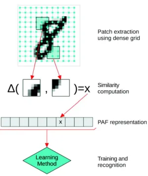
Fig. 1 The classification system based on Patch Autocorrelations Features. The PAF repre-sentation is obtained by storing the similarity between pairs of patches that are previously extracted using a dense grid over the input image. The PAF maps of train images are used to learn discriminant features. The trained classifier can then be used to predict class labels for new images represented as PAF vectors.
Algorithm 1 computes the PAF representation for a gray-scale input image I. Notice that gray-scale images are considered for simplicity, but the PAF approach can also be computed on color images. For instance, the PAF representation can be easily adapted to work on color patches. Alternatively, color images can be transformed to gray-scale before any further processing.
The following conventions and mathematical notations are considered in Al-gorithm 1 and throughout this paper. Arrays and matrices are always considered to be indexed starting from position 1, that is v = (v1, v2, ..., v|v|), where |v| is
the number of components of v. The notations vior v(i) are alternatively used to
identify the i-th component of v. The sequence 1, 2, ..., n is denoted by 1 : n, but if the step is different from the unit, it can be inserted between the lower and the upper bounds. For example, 1 : 2 : 8 generates the sequence 1, 3, 5, 7. Moreover, for a vector v and two integers i and j such that 1 ≤ i ≤ j ≤ |v|, vi:j denotes
the sub-array (vi, vi+1, ..., vj). In a similar manner, Xi:j,k:l denotes a sub-matrix
of the matrix X. Since the analyzed images are reduced to gray-scale, the notion of matrix and image can be used interchangeably, with the same meaning. In this context, a patch corresponds to a sub-matrix. The set of patches extracted from the input image is denoted by P = {P1, P2, ..., Pn}.
The first phase of Algorithm 1 (steps 10 -13) is to use a dense grid of uniformly spaced interest points in order to extract patches at a regular interval. The patches are stored in a set denoted by P. In the second phase (steps 14 -18), the patches
are compared two by two using the euclidean distance, and the distance between each pair of patches is then recorded in a specific order in the PAF vector v. More specifically, step 17 of Algorithm 1 is computed according to Equation (1). An important remark is that the features are generated in the same order for every image to ensure that all images are represented in the same way, which is a mandatory characteristic of feature representations used in machine learning. For instance, if the similarity of two patches with the origins given by the coordinate points (x, y) and (u, z) in image I, respectively, is stored at index k in the PAF vector of image I, then the similarity of the patches having the origins in (x, y) and (u, z) in any other image must always be found at index k in the PAF map. This will enable any learning method to find the discriminant features from the PAF vectors. The entire process that involves the computation of the PAF vector for image classification is illustrated in Figure 1.
A quick look at Algorithm 1 is enough to observe that the PAF approach is a simple technique. While it was found to be very effective for rather simple image classification tasks (Ionescu et al, 2015a), the PAF algorithm needs to be adjusted to handle images variations common to more complex image classification tasks. This issue is going to be addressed in the next section.
4 Translation and Rotation Invariant Patch Autocorrelation Features
Several modifications have been proposed in (Ionescu et al, 2015b) in order to transform Patch Autocorrelation Features into an approach that takes into ac-count several image variation aspects including translation and rotation changes, illumination changes, and noise. Instead of comparing the patches based on raw pixel values, a set of features is extracted from each image patch. Depending on the kind of patch features, the method can thus become invariant to different types of image variations. In this work, a set of texture-specific features are used since the approach is evaluated on the texture classification task. These features are described in detail in Section 4.1. The important remark is that a different set of features can be extracted from patches when PAF is going to be used for a different problem.
Rather than computing a single value to represent the similarity between two patches based on the extracted features, the extended PAF approach computes several similarities, one for each feature. More precisely, patches are compared using the Bhattacharyya coefficient between each of their features. Given two feature vectors fX, fY ∈ Rm extracted from two image patches X and Y , the
vector of similarity values between the two patches sX,Y is computed as follows:
sX,Y(i) =pfX(i) ·pfY(i), ∀i ∈ {1, 2, ..., m}. (2)
Note that each component of sX,Y is independently computed in the sense that
it does not depend on the other features. Therefore, sX,Y can capture different
aspects about the similarity between X and Y , since each feature can provide different information. The same features are naturally extracted from each patch, thus |fX| = |fY| = m for every pair of patches (X, Y ).
In the basic PAF approach, the next step would be to concatenate the similarity vectors generated by comparing patches two by two. This would be fine, as long as
the method relies entirely on the features to achieve invariance to different image transformations. However, further processing can be carried out to ensure that PAF remains invariant to translation and rotation, even if the extracted features are not. Unlike the basic PAF approach, the pairs of patches are vector quantized by the spatial offset between the patches of each pair. Given two patches X and Y having the origins in (x, y) and (u, z), respectively, the spatial offset o between X and Y is measured with the help of the L2 euclidean distance between their
origins:
o(X, Y ) =p(x − u)2+ (y − z)2. (3)
In order to cluster pairs of patches together, the spatial offsets are rounded to the nearest integer values. Given two pairs of patches (X, Y ) and (U, V ), they are clustered together only if ⌊o(X, Y )⌉ = ⌊o(U, V )⌉, where ⌊x⌉ is the rounding function of x ∈ R, that returns the nearest integer value to x. It is important to note that the similarity vector determined by a pair of patches is included in the cluster, not the patches themselves. Formally, a cluster (or a group) of similarity vectors between patches extracted at a given spatial offset k is defined as follows: Ck= {sPi,Pj | ⌊o(Pi, Pj)⌉ = k, ∀(Pi, Pj) ∈ P × P, 1 ≤ i < j ≤ |P|}, (4)
where P = {P1, P2, ..., P|P|} is the set of patches extracted from the input image,
o(Pi, Pj) is the offset between Pi and Pj determined by Equation (3), and sPi,Pj
is the similarity vector between patches Pi and Pj computed as in Equation (2).
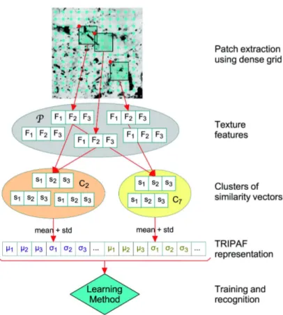
In each cluster, the similarity vectors are computed between patches that re-side at a certain spatial offset, in all possible directions. The exact position of each patch is simply disregarded in the clustering process. When the image is translated or rotated, these clusters remain mostly unaffected, because the spa-tial offsets between patches are always the same. Obviously, the patches extracted from an image will not be identical to the patches extracted from the same image after applying a rotation, specifically because the patches are extracted along the vertical and horizontal axes of the image based on a fixed grid, as illustrated in Figure 2. As such, the clusters may not contain the very same patches when the image is rotated, but in principle, each cluster should capture about the same in-formation, since the distance between patches is always preserved. Therefore, the method can be safely considered as translation and rotation invariant. The final step is to find a representation for each of these clusters. The mean and the stan-dard deviation are computed for each component of the similarity vectors within a group. Finally, the Translation and Rotation Invariant Patch Autocorrelation Features (TRIPAF) are obtained by concatenating these statistics for all the clus-ters C1, C2, ..., Cd, in this specific order, where d is a constant integer value that
determines the number of clusters. Figure 2 illustrates the entire process required for computing the TRIPAF vector.
It is important to note that in order to make sure all the images in a set I are represented by vectors of the same length, each image needs to be resized such that its diagonal is equal to the constant integer value d:
p
wI2+ hI2= d, ∀I ∈ I, (5)
where wI and hI are the width and the height of image I, respectively. The number
Fig. 2 The classification system based on Translation and Rotation Invariant Patch Auto-correlations Features. In a first stage, feature vectors are computed from patches extracted by applying a grid over the image, and then, the resulted feature vectors are stored in a set P. Then, similarity vectors are computed and subsequently clustered according to the spatial offsets between patches. Finally, the TRIPAF vector is generated by computing the mean (µ) and the standard deviation (σ) of each component of the similarity vectors within each cluster. The TRIPAF maps of train images are then used to learn discriminant features. The trained classifier can be used to predict class labels for new images represented as TRIPAF vectors. For better readability, not all arrows have been represented in this figure.
features extracted from patches and d is a positive integer value that controls the number of pairs of patches per cluster. Actually, d can be considered as a parameter of TRIPAF that can be usually adjusted in practice, in order to obtain a desired trade-off between accuracy and space. Having an extra parameter that needs to be adjusted based on empirical observations is not necessarily desired. Therefore, to reduce the number of parameters that need to be tuned, d can be set to the average diagonal size of all the images in I. An interesting detail about TRIPAF is that the clusters of similarity vectors naturally tend to become more and more sparse as the spatial offset between patches grows. Certainly, cluster C1is the most dense
cluster, while Cd contains only two components that correspond to the patches
situated in the four corners of the image. Being so far apart, the patches that form the sparse clusters no longer bring any useful information about the image.
This hypothesis was empirically tested in the context of texture classification. The accuracy of TRIPAF remains at the same level when the representation is reduced to half of its size by removing the sparse clusters Cd, Cd−1, ..., C⌊d/2⌉. Another
constant value c ∈ (0, 1] is introduced to control the proportion of dense clusters that is taken into consideration. More precisely, only the first ⌊c · d⌉ clusters will be kept in the final TRIPAF vector.
Algorithm 2:TRIPAF Algorithm
1 Input:
2 I - a gray-scale input image of h × w pixels; 3 p - the size (in pixels) of each square-shaped patch; 4 s - the distance (in pixels) between consecutive patches; 5 d - the number of clusters;
6 c - a constant value in the range (0, 1];
7 F = {F1, F2, ...., Fm | Fi: Rp× Rp→ R, ∀i} - a set of m feature extraction functions. 8 Initialization:
9 I ← resized image I such thatp(w)2+ (h)2= d; 10 (h, w) ← size(I); 11 n ← ceil((h − p + 1)/s) · ceil((w − p + 1)/s); 12 P ← ∅; 13 Ci← ∅, for i ∈ {1, 2, ..., ⌊c · d⌉}; 14 vi← 0, for i ∈ {1, 2, ..., m · ⌊c · d⌉}; 15 Computation: 16 fori = 1 : s : h do 17 forj = 1 : s : w do 18 P ← Ii:(i+p−1),j:(j+p−1); 19 fork = 1 : m do 20 fP(k) ← Fi(P ); 21 P ← P ∪ fP; 22 fori = 1 : n − 1 do 23 forj = i + 1 : n do 24 if⌊o(Pi, Pj)⌉ ≤ ⌊c · d⌉ then 25 fork = 1 : m do 26 sP i,Pj(k) ← q fPi(k) · q fPj(k); 27 C⌊o(P i,Pj)⌉← C⌊o(Pi,Pj)⌉∪ sPi,Pj; 28 k ← 1; 29 fori = 1 : ⌊c · d⌉ do 30 forj = 1 : m do 31 v(k) ← mean(s(j)), for s ∈ Ci; 32 v(k + 1) ← std(s(j)), for s ∈ Ci; 33 k ← k + 2; 34 Output:
35 v - the TRIPAF feature vector with m · ⌊c · d⌉ components.
The TRIPAF representation is computed as described in Algorithm 2. The same mathematical conventions and notations provided in Section 3 are also used in Algorithm 2. On top of these notations, two predefined functions are used to compute the mean and the standard deviation (as defined in literature), namely that is taken into consideration. More precisely, only the first ⌊c · d⌉ clusters will
mean and std. The TRIPAF algorithm can be divided into three phases. In the first phase (steps 16 -21), feature vectors are computed from patches extracted by applying a grid of uniformly spaced interest points, and then, the resulted feature vectors are stored in the set P. The notation P is used by analogy to Algorithm 1, even if it is now used to store feature vectors instead of patches. In the second phase (steps 22 -27), the similarity vectors are computed and subsequently clus-tered according to the spatial offsets between patches. In the third phase (steps 28 -33), the TRIPAF vector v is generated by computing the mean and the stan-dard deviation of each component of the similarity vectors within each cluster. A close view reveals that Algorithm 2 is more complex than Algorithm 1, but it is also more flexible, in the sense that it can easily be adapted for a variety of image classification tasks, simply by changing the set of features F . The set of texture-specific features used for the texture classification experiments are described next.
4.1 Texture Features
The mean and the standard deviation are the first two statistical features extracted from image patches. These two basic features can be computed indirectly, in terms of the image histogram. The shape of an image histogram provides many clues to characterize the image, but the features obtained from the histogram are not always adequate to discriminate textures, since they are unable to indicate local intensity differences. Therefore, more complex features are necessary.
One of the most powerful statistical methods for textured image analysis is based on features extracted from the Gray-Level Co-Occurrence Matrix (GLCM) proposed by Haralick et al (1973). The GLCM is a second order statistical measure of image variation and it gives the joint probability of occurrence of gray levels of two pixels, separated spatially by a fixed vector distance. Smooth texture gives a co-occurrence matrix with high values along diagonals for small distances. The range of gray level values within a given image determines the dimensions of a co-occurrence matrix. Thus, 4 bits gray level images give 16 × 16 co-occurrence matrices. Relevant statistical features for texture classification can be computed from a GLCM. The features proposed by Haralick et al (1973), which show a good discriminatory power, are the contrast, the energy, the entropy, the homogeneity, the variance and the correlation.
Another feature that is relevant for texture analysis is the fractal dimension. It provides a statistical index of complexity comparing how detail in a fractal pattern changes with the scale at which it is measured. The fractal dimension is usually approximated. The most popular method of approximation is box counting (Falconer, 2003). The idea behind the box counting dimension is to consider grids at different scale factors over the fractal image, and count how many boxes are filled over each grid. The box counting dimension is computed by estimating how this number changes as the grid gets finer, by applying a box counting algorithm. An efficient box counting algorithm for estimating the fractal dimension was proposed by Popescu et al (2013). The idea of the algorithm is to skip the computation for coarse grids, and count how many boxes are filled only for finer grids. The TRIPAF approach includes this efficient variant of box counting.
Daugman (1985) found that cells in the visual cortex of mammalian brains can be modeled by Gabor functions. Thus, image analysis by the Gabor functions
is similar to perception in the human visual system. A set of Gabor filters with different frequencies and orientations may be helpful for extracting useful features from an image. The local isotropic phase symmetry measure (LIPSyM) of Kuse et al (2011) takes the discrete Fourier transform of the input image, and filters this frequency information through a bank of Gabor filters. Kuse et al (2011) also note that local responses of each Gabor filter can be represented in terms of energy and amplitude. Thus, Gabor features, such as the mean-squared energy and the mean amplitude, can be computed through the phase symmetry measure for a bank of Gabor filters with various scales and rotations. These features are relevant because Gabor filters have been found to be particularly appropriate for texture representation and discrimination. The Gabor features are also used in the TRIPAF algorithm.
5 Learning Methods
There are many supervised learning methods that can be used for classification, such as Na¨ıve Bayes classifiers (Manning et al, 2008), neural networks (Bishop, 1995; Krizhevsky et al, 2012; LeCun et al, 2015), Random Forests (Breiman, 2001), kernel methods (Shawe-Taylor and Cristianini, 2004) and many others (Caruana and Niculescu-Mizil, 2006). However, all classification systems used in this work rely on kernel methods to learn discriminant patterns. Therefore, a brief overview of the kernel functions and kernel classifiers used either for handwritten digit recog-nition or texture classification is given in this section. For the texture recogrecog-nition experiments, the TRIPAF representation is combined with a bag of visual words representation to improve performance, particularly the bag of visual words rep-resentation described in (Ionescu et al, 2014b), which is based on the PQ kernel. Details about the BOVW model are also given in this section.
5.1 Kernel Methods
Kernel-based learning algorithms work by embedding the data into a Hilbert space, and searching for linear relations in that space using a learning algorithm. The embedding is performed implicitly, that is by specifying the inner product between each pair of points rather than by giving their coordinates explicitly. The power of kernel methods lies in the implicit use of a Reproducing Kernel Hilbert Space (RKHS) induced by a positive semi-definite kernel function. Despite the fact that the mathematical meaning of a kernel is the inner product in a Hilbert space, another interpretation of a kernel is the pairwise similarity between samples.
The kernel function offers to the kernel methods the power to naturally handle input data that is not in the form of numerical vectors, such as strings, images, or even video and audio files. The kernel function captures the intuitive notion of similarity between objects in a specific domain and can be any function defined on the respective domain that is symmetric and positive definite. For images, many such kernel functions are used in various applications including object recognition, image retrieval, or similar tasks. Popular choices are the linear kernel, the inter-section kernel, the Hellinger’s kernel, the χ2 kernel or the Jensen-Shannon kernel. Other state of art kernels are the pyramid match kernel of Lazebnik et al (2006) experiments, the TRIPAF representation is combined with a bag of visual words
and the PQ kernel of Ionescu and Popescu (2013a). Some of these kernels are also used in different contexts in the experiments presented in this work, specifically the linear kernel, the intersection kernel and the PQ kernel. These three kernels are described in more detail next.
For two feature vectors X, Y ∈ Rn, the linear kernel is defined as:
k(X, Y ) = hX, Y i, (6) where h·, ·i denotes the inner product.
The intersection kernel is given by component-wise minimum of the two feature vectors: k(X, Y ) = n X i min {xi, yi}. (7)
An entire set of correlation statistics for ordinal data are based on the number of concordant and discordant pairs among two variables. The number of concordant pairs among two variables X, Y ∈ Rn is:
P = |{(i, j) : 1 ≤ i < j ≤ n, (xi− xj)(yi− yj) > 0}|. (8)
In the same manner, the number of discordant pairs is:
Q = |{(i, j) : 1 ≤ i < j ≤ n, (xi− xj)(yi− yj) < 0}|. (9)
Among the correlation statistics based on counting concordant and discordant pairs are Goodman and Kruskal’s gamma, Kendall’s tau-a and Kendall’s tau-b (Upton and Cook, 2004). These three correlation statistics are very related. More precisely, all are based on the difference between P and Q, normalized differently. In the same way, the PQ kernel (Ionescu and Popescu, 2013a) between two his-tograms X and Y is defined as:
kP Q(X, Y ) = 2(P − Q). (10)
The PQ kernel can be computed in O(n log n) time with the efficient algorithm based on merge sort described in (Ionescu and Popescu, 2015). An important remark is that the PQ kernel is suitable to be used when the feature vector can also be described as a histogram. For instance, the PQ kernel improves the accuracy in object recognition (Ionescu and Popescu, 2013a, 2015) and texture classification (Ionescu et al, 2014b) when the images are represented as histograms of visual words.
After embedding the features with a kernel function, a linear classifier is used to select the most discriminant features. Various kernel classifiers differ in the way they learn to separate the samples. In the case of binary classification problems, Support Vector Machines (SVM) (Cortes and Vapnik, 1995) try to find the vector of weights that defines the hyperplane that maximally separates the images in the Hilbert space of the training examples belonging to the two classes. The SVM is a binary classifier, but image classification tasks are typically multi-class classifi-cation problems. There are many approaches for combining binary classifiers to solve multi-class problems. Usually, the multi-class problem is broken down into multiple binary classification problems using common decomposing schemes such
as one-versus-all and one-versus-one. In the experiments presented in this paper the one-versus-all scheme is adopted for SVM. Nevertheless, there are some classi-fiers that take the multi-class nature of the problem directly into account, such as Kernel Discriminant Analysis (KDA). The KDA method provides a projection of the data points to a one-dimensional subspace where the Bayes classification error is smallest. It is able to improve accuracy by avoiding the class masking problem (Hastie and Tibshirani, 2003). Further details about kernel methods can be found in (Shawe-Taylor and Cristianini, 2004).
5.2 Bag of Visual Words Model
In computer vision, the BOVW model can be applied to image classification and related tasks, by treating image descriptors as words. A bag of visual words is a vector of occurrence counts of a vocabulary of local image features. This repre-sentation can also be described as a histogram of visual words. The vocabulary is usually obtained by vector quantizing image features into visual words.
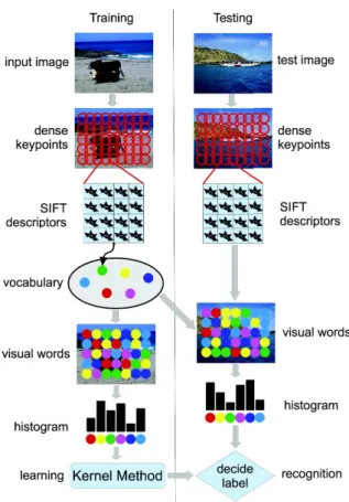
The BOVW model can be divided in two major steps. The first step is for feature detection and representation. The second step is to train a kernel method in order to predict the class label of a new image. The entire process, that involves both training and testing stages, is illustrated in Figure 3.
The feature detection and representation step works as described next. Fea-tures are detected using a regular grid across the input image. At each interest point, a SIFT feature (Lowe, 1999) is computed. This approach is known as dense SIFT (Dalal and Triggs, 2005; Bosch et al, 2007). Next, SIFT descriptors are vec-tor quantized into visual words and a vocabulary (or codebook) of visual words is obtained. The vector quantization process is done by k-means clustering (Le-ung and Malik, 2001), and visual words are stored in a randomized forest of k-d trees (Philbin et al, 2007) to reduce search cost. The frequency of each visual word in an image is then recorded in a histogram. The histograms of visual words enter the training step. Typically, a kernel method is used for training the model. In the experiments, the recently introduced PQ kernel is used to embed the features into a Hilbert space. The learning is done either with SVM or KDA, which are both described in Section 5.1.
6 Handwritten Digit Recognition Experiments
Isolated handwritten character recognition has been extensively studied in the literature (Suen et al, 1992; Srihari, 1992), and was one of the early successful applications of neural networks (LeCun et al, 1989). Comparative experiments on recognition of individual handwritten digits are reported in (LeCun et al, 1998). While recognizing individual digits is one of many problems involved in designing a practical recognition system, it is an excellent benchmark for comparing shape recognition methods.
Fig. 3 The BOVW learning model for image classification. The feature vector consists of SIFT features computed on a regular grid across the image (dense SIFT) and vector quantized into visual words. The frequency of each visual word is then recorded in a histogram. The histograms enter the training stage. Learning is done by a kernel method.
6.1 Data Set Description
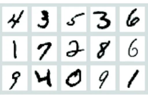
The data set used for testing the feature representation presented in this paper is the MNIST set, which is described in detail in (LeCun et al, 1998). The regular MNIST database contains 60, 000 train samples and 10, 000 test samples, size-normalized to 20 × 20 pixels, and centered by center of mass in 28 × 28 fields. A random sample of 15 images from this data set is presented in Figure 4. The data set is available at http://yann.lecun.com/exdb/mnist.
6.2 Implementation Details
The PAF representation is used in a learning context in order to evaluate its performance on handwritten digit recognition. Certainly, two learning methods based on the PAF representation are evaluated to provide a more clear overview of the performance improvements brought by PAF and to demonstrate that the improvements are not due to a specific learning method. The first classifier, that is performance on handwritten digit recognition. Certainly, two learning methods
Fig. 4 A random sample of 15 handwritten digits from the MNIST data set.
intensively used through all the experiments, is the k-Nearest Neighbors (k-NN). The k-NN classifier was chosen because it directly reflects the characteristics of the PAF representation, since there is no actual training involved in the k-NN model. A state-of-the-art kernel method is also used in the experiments, namely the SVM based on the linear kernel.
It is important to note that the TRIPAF representation is not used in the handwritten digit recognition experiments, because it is not suitable for this task. Since TRIPAF is rotation invariant, it will certainly produce nearly identical rep-resentations for some samples of digits 6 and 9, or similarly for some samples of digits 1 and 7. This means that a classifier based on the TRIPAF representation will not be able to properly distinguish these digits, consequently producing a lower accuracy rate.
6.3 Organization of Experiments
Several classification experiments are conducted using the 3-NN and the SVM classifiers based on the PAF representation. These are systematically compared with two benchmark classifiers, specifically a 3-NN model based on the euclidean distance between pixels and a SVM trained on the raw pixel representation. The experiments are organized as follows. First of all, the two parameters of PAF and the regularization parameter of SVM are tuned in a set of preliminary experiments performed on the first 300 images from the MNIST training set. Another set of experiments are performed on the first 1000 images from the MNIST training set. These subsets of MNIST contain randomly distributed digits from 0 to 9 pro-duced by different writers. The experiments on these subsets are performed using a 10-fold cross validation procedure. The procedure is repeated 10 times and the obtained accuracy rates are averaged for each representation and each classifier. This helps to reduce the variation introduced by the random selection of samples in each fold, and ensures a fair comparison between results. It is worth mentioning that the subset of 1000 images is used to assess the robustness of the evaluated methods when less training data is available. Usually, the accuracy degrades when there is less training data available, but a robust system should maintain its ac-curacy level as high as possible. Nevertheless, the classifiers are also evaluated on the entire MNIST data set. Each experiment is repeated using deslanted digits,
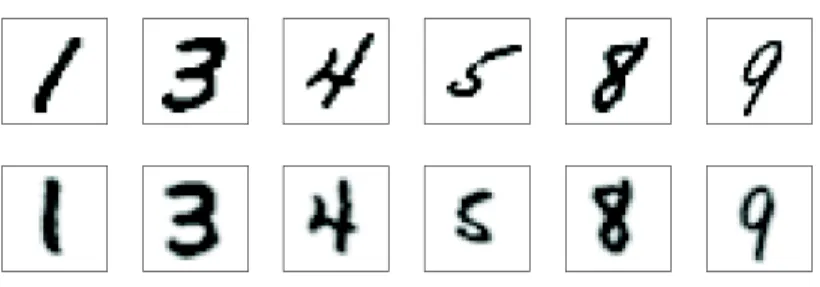
Fig. 5 A random sample of 6 handwritten digits from the MNIST data set before and after deslanting. The original images are shown on the top row and the slant corrected images are on the bottom row. A Gaussian blur was applied on the deslanted images to hide pixel distortions introduced by the deslanting technique.
which was previously reported to improve the recognition accuracy. The method used for deslanting the digits is described in Section 6.5.
6.4 Parameter Tuning
A set of preliminary tests on the first 300 images of the MNIST training set are performed to adjust the parameters of the PAF representation, such as the patch size and the pixel interval used to extract the patches. Patch sizes ranging from 1 × 1 to 8 × 8 pixels were considered. The best results in terms of accuracy were obtained with patches of 5 × 5 pixels, but patches of 4 × 4 or 6 × 6 pixels were also found to work well. In the rest of the experiments, the PAF representation is based on patches of 5 × 5 pixels.
After setting the desired patch size, the focus is to test different grid densities. Obviously, the best results in terms of accuracy are obtained when patches are extracted using an interval of 1 pixel. However, the goal of adjusting the grid density is to obtain a desired trade-off between accuracy and speed. Girds with intervals of 1 to 10 pixels were evaluated. The results indicate that the accuracy does not drop significantly when the pixel interval is less than the patch size. Consequently, a choice was made to extract patches at every 3 pixels to favor accuracy while significantly reducing the size of the PAF representation. Given that the MNIST images are 28×28 pixels wide, a grid with a density of 1 pixel generates 165.600 features, while a grid with the chosen density of 3 pixels generates only 2.016 features, which is roughly 80 times smaller.
The regularization parameter C of SVM was adjusted on the same subset of 300 images. The best results were obtained with C = 102 and, consequently, the rest of the results are reported using C = 102 for the SVM.
6.5 Deslanting Digits
A good way of improving the recognition performance is to process the images before extracting the features in order to reduce the amount of pattern variations within each class. As mentioned in (Teow and Loe, 2002), a common way of re-ducing the amount of variation is by deslanting the individual digit images. The
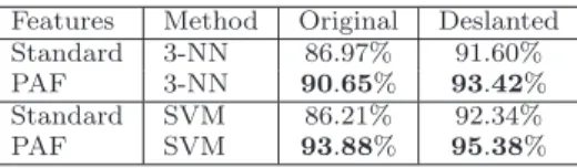
Table 1 Accuracy rates on the subset of 1000 images for the MNIST data set for the PAF representation versus the standard representation based on raw pixel data. The results are reported with two different classifiers using the 10-fold cross validation procedure. The results obtained on the original images are shown on the left-hand side and the results obtained on the deslanted images are shown on the right-hand side.
Features Method Original Deslanted Standard 3-NN 86.97% 91.60% PAF 3-NN 90.65% 93.42% Standard SVM 86.21% 92.34%
PAF SVM 93.88% 95.38%
deslanting method described in (Teow and Loe, 2002) was also adopted in this work and it is briefly described next. For each image, the least-squares regression line passing through the center of mass of the pixels is computed in the first step. Then, the image is skewed with respect to the center of mass, such that the regres-sion line becomes vertical. Since the skewing technique may distort the pixels, a slight Gaussian blur is applied after skewing. A few sample digits before and after deslanting are presented in Figure 5.
6.6 Experiment on 1000 MNIST Images
In this experiment, the PAF representation is compared with the representation based on raw pixel data using two classifiers. First of all, a 3-NN classifier based on the PAF representation is compared with a baseline k-NN classifier. The 3-NN based on the euclidean distance measure (L2-norm) between input images is the
chosen baseline classifier. In (LeCun et al, 1998) an error rate of 5.00% on the regular test set with k = 3 for this classifier is reported. Other studies (Wilder, 1998) report an error rate of 3.09% on the same experiment. The experiment was recreated in this work, and an error rate of 3.09% was obtained. Second of all, a SVM classifier based on the PAF representation is compared with a baseline SVM classifier. All the tests are conducted on both original and deslanted images.
Table 1 shows the accuracy rates averaged on 10 runs of the 10-fold cross validation procedure. The results reported in Table 1 indicate that the PAF rep-resentation improves the accuracy over the standard reprep-resentation. However, the PAF representation does not equally improve the accuracy rates for original versus deslanted images. On the original images, the PAF representation improves the accuracy of the 3-NN classifier by 3.68% and the accuracy of the SVM classifier by roughly 7.67%. In the same time, the PAF representation improves the accuracy of the 3-NN classifier by almost 2% and the accuracy of the SVM classifier by roughly 3% on the deslanted digit images. The best accuracy (95.38%) is obtained by the SVM based on the PAF map on deslanted images. First of all, the empiri-cal results presented in Table 1 show that the PAF representation is better than the standard representation for the digit recognition task. Second of all, the PAF representation together with the deslanting technique further improve the results. In conclusion, there is strong evidence that the Patch Autocorrelation Features provide a better representation for the digit recognition task.
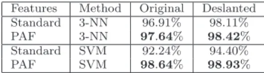
Table 2 Accuracy rates on the full MNIST data set for the PAF representation versus the standard representation based on raw pixel data. The results are reported on the official MNIST test set of 10, 000 images. The results obtained on the original images are shown on the left-hand side and the results obtained on the deslanted images are shown on the right-left-hand side.
Features Method Original Deslanted Standard 3-NN 96.91% 98.11% PAF 3-NN 97.64% 98.42% Standard SVM 92.24% 94.40%
PAF SVM 98.64% 98.93%
6.7 Experiment on the Full MNIST Data Set
The results presented in the previous experiment look promising, but the PAF vector should be tested on the entire MNIST data set for a strong conclusion of its performance level. Consequently, the 3-NN and the SVM classifiers based on the PAF representation are compared on the full MNIST data set with the 3-NN and the SVM classifiers based on the feature representation given by raw pixels values. The results are reported in Table 2.
As other studies have reported (Wilder, 1998), an error rate of 3.09% is ob-tained by the baseline 3-NN model based on the euclidean distance. The 3-NN model based on the PAF representation gives an error rate of 2.36%, which repre-sents an improvement lower than 1%. The two 3-NN models have lower error rates on deslanted images, proving that the deslanting technique is indeed helpful. The baseline 3-NN shows an improvement of 1.2% on the deslanted images. The PAF representation brings an improvement of 0.31% on the deslanted digits. Compared to the results reported in the previous experiments, the PAF representation does not have a great impact on the performance of the k-NN model. However, there are larger improvements to the SVM classifier. The PAF representation improves the accuracy of the SVM classifier by 6.4% on the original images, and by 4.53% on the deslanted images. Overall, the PAF representation seems to have a signif-icant positive effect on the performance of the evaluated learning methods. The lowest error rate on the official MNIST test set (1.07%) is obtained by the SVM based on Patch Autocorrelation Features. This performance is similar to those reported by state-of-the-art models such as virtual SVM (DeCoste and Sch¨olkopf, 2002), boosted stumps (K´egl and Busa-Fekete, 2009), or deep Boltzmann ma-chines (Salakhutdinov and Hinton, 2009). In conclusion, the PAF representation can boost the performance of the 3-NN and the SVM up to state-of-the-art accu-racy levels on the handwritten digit recognition task, with almost no extra time required. Indeed, it takes 20 milliseconds on average to compute the PAF rep-resentation for a single MNIST image on a machine with Intel Core i7 2.3 GHz processor and 8 GB of RAM using a single Core. Hence, the method can even be used in real-time applications.
7 Texture Classification Experiments
Texture classification is a difficult task, in which methods have to take into account several aspects such as translation, rotation, and scale variations, illumination -NN model. However, there are larger improvements to the SVM classifier. The PAF representation improves
Fig. 6 Sample images from three classes of the Brodatz data set.
changes, viewpoint changes, and non-rigid distortions. Thus, texture classification is an adequate task to prove that a particular method is robust to such image vari-ations. Indeed, the main goal of the texture classification experiments presented in this section is to demonstrate that TRIPAF is invariant to several image trans-formations, including translation and rotation changes, and that it can yield good results on this rather difficult image classification task.
7.1 Data Sets Description
Texture classification experiments are presented on two benchmark data sets of texture images. The first experiment is conducted on the Brodatz data set (Bro-datz, 1966). This data set is probably the best known benchmark used for texture classification, but also one of the most difficult, since it contains 111 classes with only 9 samples per class. The standard procedure in the literature is to obtain samples of 213 × 213 pixels by cutting them out from larger images of 640 × 640 pixels using a 3 by 3 grid. Figure 6 presents three sample images per class of three classes randomly selected from the Brodatz data set.
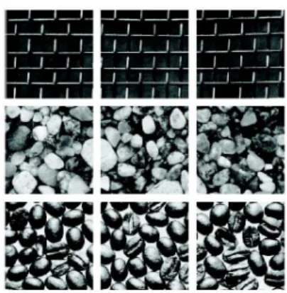
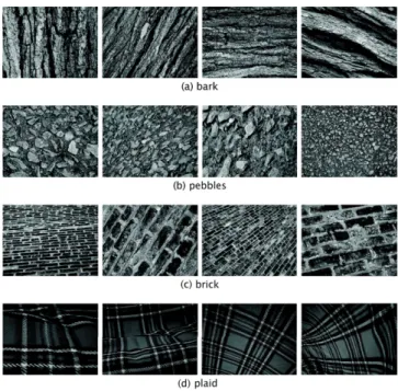
The second experiment is conducted on the UIUCTex data set of Lazebnik et al (2005). It contains 1000 texture images of 640 × 480 pixels representing different types of textures such as bark, wood, floor, water, and more. There are 25 classes of 40 texture images per class. Textures are viewed under significant scale, viewpoint and illumination changes. Images also include non-rigid deformations. This data set is available for download at http://www-cvr.ai.uiuc.edu/ponce grp. Figure 7 presents four sample images per class of four classes representing bark, brick, pebbles, and plaid.
7.2 Implementation Details
The TRIPAF representation is compared with a method that extracts texture-specific features from entire images, on the texture classification task. Among the GLCM features that show a good discriminatory power, only four of them are used
Fig. 7 Sample images from four classes of the UIUCTex data set. Each image is showing a textured surface viewed under different poses.
by the classification systems, namely the contrast, the energy, the homogeneity, and the correlation. These GLCM features are averaged on 4 directions (vertical, horizontal and diagonals) using gaps of 1 and 2 pixels. The mean and the standard deviation are also added to the set of texture-specific features. Another feature is given by the box counting dimension. The Gabor features (the mean-squared energy and the mean amplitude) are computed on 3 scales and 6 different rotations, resulting in a total of 36 Gabor features (2 features × 3 scales × 6 directions). There are 43 texture-specific features put together. Alternatively, the two Gabor features are also averaged on 3 scales and 6 different rotations, generating only 4 Gabor features. This produces a reduced set of 9 texture-specific features, which is more robust to image rotations and scale variations. Results are reported using both representations, one of 43 features and the other of 9 features.
The parameter d that determines the number clusters in the TRIPAF approach was set to the average diagonal size of the images in each data set. Without any tuning, the parameter c was set to 0.5 in order to reduce the size of the TRIPAF map by half. As a consequence, all the TRIPAF representations have between 300 and 1500 components.
The TRIPAF approach, which is rotation and translation invariant, is com-bined with the BOVW model, which is scale invariant (due to the SIFT descrip-tors), in order to obtain a method that is invariant to all affine transformations. These methods are combined at the kernel level through multiple kernel learning (MKL) (Gonen and Alpaydin, 2011). When multiple kernels are combined, the features are actually embedded in a higher-dimensional space. As a consequence,
the search space of linear patterns grows, which helps the classifier to select a better discriminant function. The most natural way of combining two kernels is to sum them up, and this is exactly the MKL approach used in this paper. Summing up kernels in the dual form is equivalent to feature vector concatenation in the primal form. The combined representation is alternatively used with the SVM or the KDA. The two classifiers are compared with other state-of-the-art approaches (Zhang et al, 2007; Nguyen et al, 2011; Quan et al, 2014), although Quan et al (2014) do not report results on the Brodatz data set.
7.3 Parameter Tuning
A set of preliminary tests on a subset of 40 classes from Brodatz are performed to adjust the parameters of the PAF representation, such as the patch size, and the pixel interval used to extract the patches. Patches of 16 × 16, 32 × 32 and 64 × 64 pixels were considered. Better results in terms of accuracy were obtained with either patches of 16 × 16 or 32 × 32 pixels, and the rest of the experiments are based on patches of such dimensions. The TRIPAF representations generated by patches of 16 × 16 or 32 × 32 pixels are also combined by summing up their kernels to obtain a more robust representation.
After setting up the patch sizes, the next goal is to adjust the grid density. The grid density was chosen such that the processing time of TRIPAF is less than 5 seconds per image on a machine with Intel Core i7 2.3 GHz processor and 8 GB of RAM using a single Core. Notably, more than 90% of the time is required to extract the texture-specific features from every patch. For the Brodatz data set, patches are extracted at an interval of 8 pixels, while for the UIUCTex data set, patches are extracted at every 16 pixels.
The regularization parameter C of SVM was adjusted on the same subset of of 40 classes from Brodatz. The best results were obtained with C = 104 and, consequently, the rest of the results are reported using C = 104 for the SVM. In a similar fashion, the regularization parameter of KDA was set to 10−5.
7.4 Experiment on Brodatz Data Set
Typically, the results reported in previous studies (Lazebnik et al, 2005; Zhang et al, 2007; Nguyen et al, 2011) on the Brodatz data set are based on randomly selecting 3 training samples per class and using the rest for testing. Likewise, the results presented in this paper are based on the same setup with 3 random samples per class for training. Moreover, the random selection procedure is repeated for 20 times and the resulted accuracy rates are averaged. This helps to reduce the amount of accuracy variation introduced by using a different partition of the data set in each of the 20 trials. To give an idea of the amount of variation in each trial, the standard deviations for the computed average accuracy rates are also reported. The evaluation procedure described so far is identical to the one used in the state-of-the-art approaches (Zhang et al, 2007; Nguyen et al, 2011) that are included in the following comparative study.
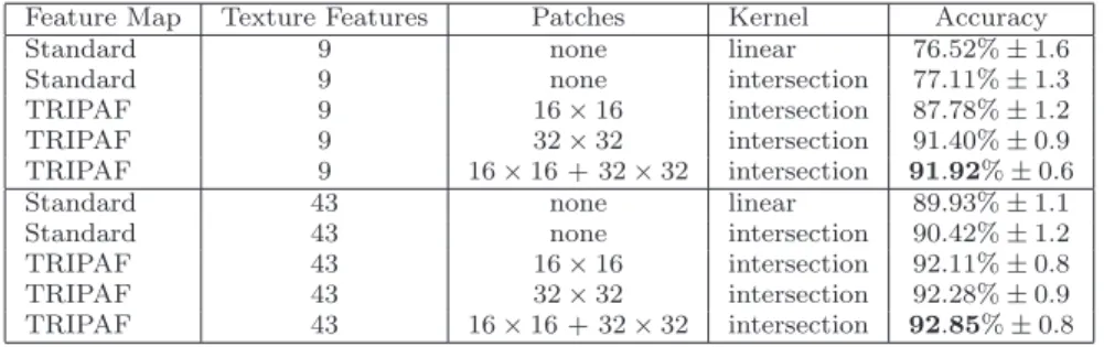
Table 3 presents the accuracy rates of the SVM classifier based on several TRIPAF representations, in which the number of texture-specific features and
Table 3 Accuracy rates of the SVM classifier on the Brodatz data set for the TRIPAF repre-sentation versus the standard reprerepre-sentation based on texture-specific features. The reported accuracy rates are averaged on 20 trials using 3 random samples per class for training and the other 6 for testing. The best accuracy rate for each set of texture-specific features is highlighted in bold.
Feature Map Texture Features Patches Kernel Accuracy
Standard 9 none linear 76.52% ± 1.6
Standard 9 none intersection 77.11% ± 1.3
TRIPAF 9 16 × 16 intersection 87.78% ± 1.2
TRIPAF 9 32 × 32 intersection 91.40% ± 0.9
TRIPAF 9 16 × 16 + 32 × 32 intersection 91.92% ± 0.6
Standard 43 none linear 89.93% ± 1.1
Standard 43 none intersection 90.42% ± 1.2
TRIPAF 43 16 × 16 intersection 92.11% ± 0.8 TRIPAF 43 32 × 32 intersection 92.28% ± 0.9 TRIPAF 43 16 × 16 + 32 × 32 intersection 92.85% ± 0.8
Table 4 Accuracy rates of the TRIPAF and BOVW combined representation on the Brodatz data set compared with state-of-the-art methods. The TRIPAF representation is based on 43 texture-specific features extracted from patches of 16 × 16 and 32 × 32 pixels. The BOVW model is based on the PQ kernel. The reported accuracy rates are averaged on 20 trials using 3 random samples per class for training and the other 6 for testing. The best accuracy rate is highlighted in bold.
Model Accuracy
SVM based on BOVW (Ionescu et al, 2014b) 92.94% ± 0.8 SVM based on TRIPAF 92.85% ± 0.8 SVM based on TRIPAF + BOVW 96.24% ± 0.6 KDA based on TRIPAF + BOVW 96.51% ± 0.7 Best model of Zhang et al (2007) 95.90% ± 0.6 Best model of Nguyen et al (2011) 96.14% ± 0.4
the size of the patches are varied. Several baseline SVM classifiers, based on the same texture-specific features used in the TRIPAF representation, are included in the evaluation in order to estimate the performance gain offered by TRIPAF. When the set of 9 texture-specific features is being used, the TRIPAF approach improves the baseline by more than 10% in terms of accuracy. On the other hand, the difference is roughly 2% in favor of TRIPAF when the set of 43 texture-specific features is being used. Both the standard and the TRIPAF representations work better when more texture-specific features are extracted, probably because the Brodatz data set does not contain significant rotation changes within each class of images. Nevertheless, the TRIPAF approach is always able to give better results than the baseline SVM. An interesting remark is that the results of TRIPAF are always better when patches of 16 × 16 pixels are used in conjunction with patches of 32 × 32 pixels, even if the accuracy improvement over using them individually is not considerable (below 1%). The best accuracy (92.85%) is obtained by the SVM based on the TRIPAF approach that extracts 43 features from patches of 16 × 16 and 32 × 32 pixels.
The empirical results presented in Table 3 clearly demonstrate the advantage of using the TRIPAF feature vectors. Intuitively, further combining TRIPAF with BOVW should yield even better results. While TRIPAF is rotation and translation
Table 5 Accuracy rates of the SVM classifier on the UIUCTex data set for the TRIPAF representation versus the standard representation based on textuspecific features. The re-ported accuracy rates are averaged on 20 trials using 20 random samples per class for training and the other 20 for testing. The best accuracy rate for each set of texture-specific features is highlighted in bold.
Feature Map Texture Features Patches Kernel Accuracy
Standard 9 none linear 78.23% ± 1.7
Standard 9 none intersection 79.87% ± 1.3
TRIPAF 9 16 × 16 intersection 92.60% ± 1.1
TRIPAF 9 32 × 32 intersection 92.38% ± 1.1
TRIPAF 9 16 × 16 + 32 × 32 intersection 93.54% ± 1.1
Standard 43 none linear 82.19% ± 1.6
Standard 43 none intersection 83.62% ± 1.4
TRIPAF 43 16 × 16 intersection 91.40% ± 1.2 TRIPAF 43 32 × 32 intersection 90.91% ± 1.2 TRIPAF 43 16 × 16 + 32 × 32 intersection 91.82% ± 1.0
invariant, BOVW is scale invariant, and therefore, these two representations com-plement each other perfectly. Table 4 compares the results of TRIPAF and BOVW combined through MKL with the results of two state-of-the-art methods (Zhang et al, 2007; Nguyen et al, 2011). The intersection kernel used in the case of TRIPAF is summed up with the PQ kernel used in the case of BOVW (Ionescu et al, 2014b). The individual results of TRIPAF and BOVW are also listed in Table 4. The two methods obtain fairly similar accuracy rates when used independently, but the accuracy rates are almost 3% lower than the state-of-the-art methods. However, the kernel combination of TRIPAF and BOVW yields results comparable to the state-of-the-art methods (Zhang et al, 2007; Nguyen et al, 2011). In fact, the best accuracy rate on the Brodatz data set (96.51%) is given by the KDA based on TRIPAF and BOVW, although the SVM based on the kernel combination is also slightly better than both state-of-the-art models. The kernel sum of TRIPAF and BOVW is much better than using the two representations individually, proving that the idea of combining them up is indeed crucial for obtaining state-of-the-art results.
7.5 Experiment on UIUCTex Data Set
As in the previous experiment, the standard evaluation procedure for the UIUC-Tex data set is used to assess the performance of approach proposed in this work. More precisely, the samples are split into a training set and a test set by ran-domly selecting 20 samples per class for training and the remaining 20 samples for testing. The random selection process is repeated for 20 times and the resulted accuracy rates are averaged over the 20 trials. Table 5 reports the average accu-racy rates along with their standard deviations which give some indication about the amount of variation in each trial. In Table 5, the SVM classifiers based on various TRIPAF representations are compared with baseline SVM classifiers that extract the same texture-specific features used in the TRIPAF representation, but from entire images instead of patches. For each set of texture-specific features, the TRIPAF approach improves the baseline by roughly 10%. It can be observed that the improvement is higher for the set of 9 texture-specific features, going up by