THÈSE
THÈSE
En vue de l'obtention duDOCTORAT DE L’UNIVERSITÉ DE TOULOUSE
DOCTORAT DE L’UNIVERSITÉ DE TOULOUSE
Délivré par l'Université Toulouse III - Paul Sabatier Discipline ou spécialité : Physique de l'Atmosphère
Présentée et soutenue par Oscar Arnoud VAN DER VELDE Le jeudi 21 février 2008
Titre :
Morphologie de sprites et conditions de productions de sprites et de jets
dans les systèmes orageux de méso-échelle
JURY
Serge CHAUZY Professeur, Université Toulouse III Président Martin FÜLLEKRUG Senior Scientist, Université de Bath (GB) Rapporteur Pierre LAROCHE Ingénieur Chercheur, ONERA Rapporteur Elisabeth BLANC Directrice de Recherche, CEA Examinateur Torsten NEUBERT Senior Scientist, National Space Institute (DK) Examinateur Joan MONTANYÀ Prof. associé, Univ. Polytechnique de Catalogne Membre invité Serge SOULA Physicien OMP, Université Toulouse III Directeur de thèse
Ecole doctorale : Sciences de l'Univers, de l'Environnement et de l'Espace (SDU2E) Unité de recherche : Laboratoire d'Aérologie
Directeur(s) de Thèse : Serge SOULA
Photo: Photo: Photo:
Photo: A “jellyfish” red sprite, photographed by the author with a Canon EOS 350D modified to pass infrared light. It occurred in the evening of 8 October 2009, at 21:43:54 UT and was triggered by a lightning flash 8 km ENE of Nant, southern France, at a distance of 290 km from the location of observation (Sant Vicenç de Castellet in northeastern Spain). Settings: ISO 1600, 0.3 seconds at f/1.6, 50 mm lens, RAW.
Remerciements
My first thanks go to Serge Soula, my Directeur de Thèse, for his support and patience (waiting for me to deposit the final thesis document, now three years after the Soutenance!). Thank you for everything Serge, and we sure will keep working together on new articles for the years to come! At the Laboratoire I enjoyed also the lunch conversations with Serge Chauzy, and I am thankful to my office-mate Marie-Pierre, who also was a great company for my cat at the office when I was on holiday! I really appreciate the help all three of you provided me.
Second, I'd like to acknowledge everyone who made possible the EU FP5 research training network “Coupling of Atmospheric Layers” (CAL), which provided us with an extremely interesting research topic and funding. In particular, thank you Torsten Neubert, not only for your organizing work which made it all possible but also for making it a big success and establishing a strong bond between European research groups, of which I still reap the benefits today (and surely not only me). I am grateful also to the rest of the Danish Space Center team for the observations infrastructure and resulting data which provided the basis of this dissertation.
The CAL community felt like a warm, comfortable home to me, with stimulating interactions and informal activities with “senior” scientists as well as my fellow “Young Scientists”, which were very welcome, because in Toulouse we were the only two persons investigating sprites! With the same joy I look back at the inspiring and fruitful interactions with my colleagues overseas, as well as the short term mission (COST P18 Lightning) in the Israeli sprite group. I'm already looking forward to meeting all of you again!
I'd like to take also the opportunity here to express my gratitude, gladly one more time, to the anonymous reviewers for their efforts of constructively reviewing (and thereby indeed improving) the submitted journal articles of my dissertation work.
Furthermore, I am grateful to Joan Montanyà for managing a smooth transition for me between Toulouse and my new position in the Lightning Research Group of the Technical University of Catalonia, as part of the new ESA Atmosphere-Space Interactions Monitor (ASIM) project, which follows up CAL.
And finally, a warm thank you to my friends, distant or by my side, who I have seen once a year or every day, and to my parents, brothers and other family in The Netherlands. A happy life with fun besides this thesis was not possible without you!
Table des Matières
1 Introduction générale ... 7
2 Scientific context ... 10
2.1 INTRODUCTION ...10
2.2 EARTH-ATMOSPHERE ELECTRIC CIRCUIT ...11
2.3 TRANSIENT LUMINOUS EVENTS ...12
2.3.1 SPRITES ...12
2.3.2 HALOS ...23
2.3.3 ELVES ...24
2.3.4 JETS ...26
2.4 THUNDERSTORMS ...31
2.4.1 METEOROLOGYOFDEEP MOISTCONVECTION ...31
2.4.2 THUNDERSTORMELECTRIFICATION ...34
2.4.3 MESOSCALE CONVECTIVE SYSTEMS ANDTHEIRELECTRICAL ASPECTS ...39
2.5 LIGHTNING ...45
2.5.1 LIGHTNINGINITIATION ...45
2.5.2 INTRACLOUDFLASHES ...46
2.5.3 CLOUD-TO-GROUND FLASHES ...49
2.6 INSTRUMENTATION ...52
2.6.1 SPRITE OBSERVATIONSYSTEMS ...52
2.6.2 RADAR ...55
2.6.3 MÉTÉORAGE CG LIGHTNING DETECTION NETWORK ...55
2.6.4 SAFIR INTRACLOUD LIGHTNING DETECTION SYSTEM ...56
2.6.5 ELF/VLF ELECTROMAGNETIC MEASUREMENTS ...58
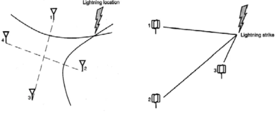
2.7 GEOMETRICAL CALCULATIONS ...59
2.7.1 ALTITUDEOFA TLE ABOVETHE EARTH’SSURFACE ...59
2.7.2 GREAT CIRCLE PATHS ...62
2.7.3 TRIANGULATIONOF GREAT CIRCLE PATHS ...64
3 Observation des relations entre la morphologie des sprites et les processus
intra-nuageux de l’éclair parent ... 78
3.1 RÉSUMÉ ...78
3.2 ARTICLE ...83
4 Analyse d’orage et d’activité d’éclair associés à des sprites observés
pendant la campagne EuroSprite: 2 cas d’étude ... 92
4.1 RÉSUMÉ ...92
4.2 ARTICLE ...97
5 Evolution spatio-temporelle de décharges de grande extension horizontale
et associées à des éclairs positifs producteurs de sprite dans le Nord de
l’Espagne ... 113
5.1 RÉSUMÉ ...113
5.2 ARTICLE ...118
6 Etudes statistiques des relations entre sprites et leur morphologie, éclair et
précipitation ... 136
6.1 RÉSUMÉ ...136
6.2 ARTICLE ...142
7 Analyse du premier Jet Géant observé au-dessus du continent
Nord-Américain ... 182
7.1 RÉSUMÉ ...182
7.2 ARTICLE ...186
Figure Figure Figure
Figure 1111. Overview of the family of Transient Luminous Events and their typical position over a. Overview of the family of Transient Luminous Events and their typical position over a. Overview of the family of Transient Luminous Events and their typical position over a. Overview of the family of Transient Luminous Events and their typical position over a
thunderstorm: blue jets, gigantic jets, pixies, trolls, sprites, elves and halos. Image courtesy of Walter Lyons thunderstorm: blue jets, gigantic jets, pixies, trolls, sprites, elves and halos. Image courtesy of Walter Lyonsthunderstorm: blue jets, gigantic jets, pixies, trolls, sprites, elves and halos. Image courtesy of Walter Lyons thunderstorm: blue jets, gigantic jets, pixies, trolls, sprites, elves and halos. Image courtesy of Walter Lyons (except kite).
(except kite).(except kite). (except kite).
1
Introduction générale
Le terme TLE est maintenant évoqué couramment dans la communauté scientifique en physique de l’environnement. Littéralement de l’anglais Transient Luminous Event, il désigne des phénomènes lumineux transitoires qui se produisent au-dessus des orages sur plusieurs dizaines de km de hauteur et dont on connaît l’existence depuis environ 18 ans. C’est en effet en 1989 et en testant une caméra sensible, qu’une équipe de l’Université du Minnesota obtint une image montrant une émission lumineuse de courte durée dans la direction d’un orage qui se trouvait derrière l’horizon (Franz et al., 1990). Cette première observation d’une longue série était un cas de "red sprite", un de ces TLEs qui apparaît au-dessus des orages de grande taille et qui maintenant a été détecté dans toutes les régions du monde. Des témoignages, notamment de pilotes, avaient bien indiqué des brefs éclairs de forme et couleur très variées visibles à l’œil nu au-dessus des orages, mais le risque qu’ils pouvaient représenter pour leur crédibilité professionnelle fait qu’ils préféraient souvent ne rien déclarer du tout. Parmi toutes ces observations, certaines correspondaient aussi à des éclairs qui semblaient se développer verticalement à partir du nuage et qui allaient être confirmées un peu plus tard en 1994 avec la découverte des "blue jets" sous la forme de décharges coniques par une équipe de l’Université d’Alaska au cours de vols autour d’orages dans l’état de l’Arkansas aux USA (Wescott et al. 1995). Certains avaient même un tel développement vertical qu’ils ont pris le nom de "gigantic jets" découverts en 2002 pendant une campagne à Porto Rico (Pasko et al. 2002). En fait, ces phénomènes relient électriquement le sommet du nuage d’orage à la couche inférieure de l’ionosphère qui se trouve la nuit à une altitude d’environ 80 km. Les observations se sont étendues à partir d’engins spatiaux et en 1995, on a augmenté la diversité du phénomène avec un nouveau membre constitué par les "elves", sortes de cercle lumineux à la base de l’ionosphère plus facile à observer depuis l’espace aux limbes de la Terre (Fukunishi et al. 1996). Ces TLEs sont liés à des champs électriques ou à des impulsions électro-magnétiques générés par les orages. Il reste un certain nombre de questions sans réponse autour de ces phénomènes, notamment le taux de production global et la relation précise entre l’éclair et le sprite. Aussi, des campagnes d’observation depuis le sol, associant de plus en plus de moyens pour caractériser l’ensemble des processus mis en jeu, se font régulièrement sur plusieurs continents et à des saisons différentes de l’année. Plusieurs projets spatiaux d’étude de ces phénomènes sont soit en cours (ISUAL au Japon) soit en préparation (TARANIS, ASIM en Europe).
La découverte de ces TLEs mais aussi des Flashs Gamma d’origine Terrestres (TGFs) a révolutionné notre compréhension de l’environnement de la Terre en révélant une occurrence importante de transferts d’énergie impulsifs entre la troposphère et les couches supérieures de l’atmosphère. L’énergie totale dissipée par ces événements pris individuellement est de l’ordre de dizaines de Mégajoules et les puissances mises en jeu se comptent en Gigawatts. Les énergies des électrons intervenant dans les décharges électriques varient de quelques eV à des dizaines de MeV en produisant des émissions dans
l’ensemble du spectre électromagnétique. L’impact de ces phénomènes est loin d’être compris, ils affectent l’équilibre chimique de l’atmosphère (ozone et oxydes d’azote), le circuit électrique global de la Terre et perturbent les ceintures de radiation. Les mécanismes source font l’objet de nombreuses discussions, ils font intervenir des processus physiques qui n’avaient pas été envisagés jusqu’à présent et qui pourraient avoir des implications plus larges et se manifester dans d’autres environnements planétaires. Aussi la recherche sur ces phénomènes a rassemblé des scientifiques d’horizons divers (physique de la décharge, physique de l’atmosphère, chimie de l’environnement, physique du rayonnement, structure de l’ionosphère, etc.). Le projet européen CAL en est un exemple. De 2002 à 2006, il a réuni plusieurs équipes de scientifiques avec notamment des spécialistes de la décharge, des spécialistes de la physique de l’orage, des spécialistes de l’ionosphère, des chimistes de la haute-atmosphère, afin de mieux déterminer les mécanismes à l’origine des TLEs (Neubert et al., 2005). Les principaux objectifs du projet étaient de comprendre leurs conditions d’occurrence, de déterminer leurs taux, de caractériser les processus physiques de leur déclenchement et de préciser leur impact sur l’ionosphère et leur rôle dans la chimie de l’atmosphère. Le laboratoire d’Aérologie a participé aux travaux dans le cadre de ce projet, d’une part pour l’analyse des caractéristiques de l’orage et de son activité associés à la production de sprites et d’autre part pour leur observation avec des systèmes utilisant des caméras sensibles. Mon rôle a été de traiter les données de la première campagne faite en 2003 dans le cadre de CAL en associant des données radar météorologique pour la structure des orages, des données satellite météosat canal infrarouge pour la hauteur du sommet des nuages, des données de détection d’éclairs issues de plusieurs types de systèmes pour avoir une vue la plus complète possible sur l’activité d’éclair associée aux sprites. Mes premiers résultats ont été intégrés dans un article collectif présentant la campagne et ses résultats préliminaires. J’ai développé des collaborations lors de cette première étape qui a fait l’objet d’un article que l’on retrouvera dans le chapitre 3 de ce document. J’ai par la suite participé à l’organisation de nouvelles campagnes et j’ai développé un système complet pour l’enregistrement de signatures de phénomènes lumineux utilisé à partir de l’été 2006. Après de nouvelles observations, une étude particulière a porté sur un cas de sprite déplacé par rapport à son éclair parent afin de donner une explication à ces observations déjà commentées dans la littérature mais pas clairement interprétées. Le chapitre 5 du document expose cette étude sous la forme d’un article. L'article a été élargie avec une analyse approfondie des nouvelles observations en 2008. J’ai réalisé une étude statistique basée sur un nombre important de cas recensés sur plusieurs campagnes (2003, 2005 et 2006) et portant sur les caractéristiques des éclairs produisant des sprites et sur celles de ces mêmes sprites, abordant des aspects tout à fait nouveaux. Elle est incluse dans le chapitre 6 du document. Afin de caractériser la nature d’orages produisant des sprites, leur évolution et l’activité d’éclair typique à plusieurs échelles de temps, deux études de cas ont été développées de façon complète et sont présentées dans un article que l’on trouvera dans le chapitre 4 du document. Enfin, j’ai réalisé à mon initiative personnelle et en collaboration avec des chercheurs américains, l’étude des conditions de production d’un jet géant observé dans le Texas aux USA. Un article publié sur cette étude constitue le chapitre 7 du document. Le chapitre 2 du document est une large description des connaissances sur les TLEs, sur les
phénomènes en amont que sont les orages et sur les moyens d’observation dont les données ont été utilisées au cours de mon travail de thèse.
2
Scientific context
2.1
Introduction
The mysterious sounding “Red Sprites” are luminous phenomena high above thunderstorms in the mesosphere that have not been discovered until only recently. In 1989, a team of the University of Minnesota tested a new low-light camera system intended for research of the aurora, and recorded short-lasting pillars of light in the direction of a thunderstorm that was below the horizon (Franz et al, 1990).
This was a late discovery, considering that sprites are now observed as a common occurrence over large thunderstorm systems, that they are much brighter than for example the far dwarf planet Pluto (discovered in 1930!) and that they occur almost everywhere on our own planet!
Not surprisingly, eye-witness accounts of variously-shaped and colored brief flashes above storms have accumulated over more than a century, many of pilots who frequently fly in the clear air around thunderstorms – who were afraid they may not be taken seriously “seeing things”. The reports also included strange upward lightning events, of which the first scientific proof was obtained in 1994, when a team of sprite researchers from the University of Alaska flew around thunderstorms in the state of Arkansas and found conical discharges escaping from the top of thunderclouds, now known as “blue jets” (Wescott et al. 1995). A similar but bigger new phenomenon dubbed “gigantic jet” was discovered in 2002 during an experiment in Puerto Rico (Pasko et al. 2002), and in the same year from Taiwan (Su et al. 2003). These events bridge the entire distance between the cloud tops and the lower regions of the ionosphere, around 80 kilometers altitude.
Not only from the ground or from airplanes, but also from spacecraft sprites and jet-like phenomena have been observed, as well yet another type of “Transient Luminous Event” (TLE): “elves”, discovered in 1995 (Fukunishi et al. 1996). These are rings of light at the base of the ionosphere, and easier to detect from space over the Earth limb.
The entire family of known TLEs is related to electric fields and electromagnetic pulses generated in thunderstorms, and the conductivity between thunderstorm and ionosphere. They serve a yet unknown role in the electric circuit of the Earth and may also affect atmospheric layers chemically (NOx and ozone production). Sprites are a real world example of low pressure streamer discharges, and have sparked the interest of scientists from many different disciplines.
During the pilot project EuroSprite2000 (Neubert et al. 2001) sprites were captured over Europe for the first time by a camera installed on Pic du Midi de Bigorre (2877 m) in the Pyrenees. This success provided the basis for cooperation between various research groups in Europe interested in different aspects of sprites, united by the European Union Research Training Network “Coupling of Atmospheric Layers” (CAL) in 2002 for a period
of four years. The EuroSprite campaigns of 2003, 2005 and 2006 were a logical follow-up and provided the data used for the studies in this thesis. Neubert et al. (2005) presented an overview of the scope and the first results of the CAL network. Under CAL working program WP5, the objective of this thesis is to gain better understanding of the conditions in thunderstorms and processes in lightning that are at the basis of the occurrence of sprites and jets.
2.2
Earth-atmosphere electric circuit
The ionosphere is a region of the upper atmosphere where the air is ionized by radiation from the sun. It spans from the magnetosphere down to exosphere, thermosphere and into the upper half of the mesosphere. The height at which ionization is significant depends on diurnal, seasonal and 11-year solar activity cycles and is lower towards the poles. The ionosphere ‘starts’ around 50 km altitude during the day, and around 80 km at night.
As ion density decreases with altitude, the path length of free electrons increases before recombination of electrons (or negative ions) with positive ions occurs. This gives the ionosphere properties of a conductor for electric currents, and therefore functions together with the conducting surface of the Earth as capacitor plates in the Earth’s electric circuit.
Within the circuit, thunderstorms fulfill the role of batteries, maintaining the difference of electric potential (Wilson, 1920). As the average thunderstorm top contains positive charge and the lower parts negative charge, brought to Earth by negative cloud to ground flashes and precipitation, the ionosphere is on average at a positive 250 kV potential compared to the Earth, but most of the potential difference is contained in the lowest kilometers of the troposphere, where positive space charge accumulates due to low mobility. So, while conductivity suggests that the ionosphere works as the outer shell of a spherical capacitor, with the surface of the Earth as inner shell, most of the charge in this circuit is present between these shells in the planetary boundary layer and in electrified precipitation.
The DC fair weather electric field near the surface is about -100 V/m, which exhibits diurnal fluctuations known as the Carnegie curve. It shows a peak during the local afternoons of the most thundery parts of the planet (Africa and South America) which have the strongest contribution in charging up the circuit by negative cloud-to-ground flashes. Conduction currents flow between the ionosphere and the surface, consisting of positive ions moving downwards and negative ions upwards.
2.3
Transient Luminous Events
2.3.1 Sprites
General characteristics
Sprites are streamer discharges occurring in the mesosphere above thunderstorms, lasting no longer than the blink of an eye. Sprites develop in tight connection to particularly intense lightning discharges which precede them by several milliseconds to more than two hundred milliseconds (Boccippio et al. 1995). Instead of rising out of a thunder cloud, they develop in mid-air usually between 50 and 90 kilometers altitude (Sentman et al. 1995), with the brightest part between 65 and 75 km. Individual streamers at the low pressures where sprites occur are tens of meters wide (Gerken et al. 2000) and a typical sprite element is 5-15 kilometers wide. Large sprites can span 50-100 km horizontally.
Figure Figure Figure
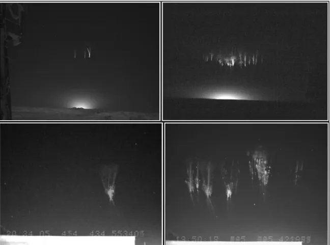
Figure 2222. Examples of classic columniform sprites (top row) and carrot sprites (bottom row). Banding. Examples of classic columniform sprites (top row) and carrot sprites (bottom row). Banding. Examples of classic columniform sprites (top row) and carrot sprites (bottom row). Banding . Examples of classic columniform sprites (top row) and carrot sprites (bottom row). Banding artifacts are caused by video interlacing.
artifacts are caused by video interlacing.artifacts are caused by video interlacing. artifacts are caused by video interlacing.
There can be a lot of variation among sprites even within a few hours of observations, especially in vertical and horizontal dimensions, number of elements (groups), brightness and fine details. The most elementary sprite is a luminous column with a slightly diffuse top and abrupt bottom, from which dim streamers may stretch downward (Wescott et al., 1998a). They tend to cluster in groups, in rare cases as large as thirty elements. Carrot sprites have a bright body (or ‘head’) usually containing beads, from which long, usually dendritically shaped lower tendrils stretch out downward, and more wispy ‘hairs’ stretch out upward. Characteristic of most sprites are a diffuse region at the top, with streamers stretching downward (Pasko and Stenbaek-Nielsen, 2002).
Single elements develop within the time of a standard video frame (16 milliseconds), but a sprite event may consist of several elements that may dance above a thunderstorm occasionally for longer than 100 milliseconds (Lyons, 1994, 1996). The initial movement of streamers of normal sprites is downward (Stanley et al. 1999, McHargh et al. 2002, 2007). The upward-directed negative streamers appear to start from existing luminous structures from lower altitudes than the initial development, clearly visible in very-high speed (10 000 frames per second) imagery obtained by Stenbaek-Nielsen et al. (2007). The same recordings show that the streamers seen in normal images are just the traces of actually very bright streamer heads: wave fronts of ionization emitting light brighter than the planet Venus. Unfortunately, due to their fast movement (107 m s-1) for a fraction of a second, sprites barely make a lasting impression to the eye.
Eye-witnesses reported different colors over the decennia, confirmed by observations of Lyons (1996) who found that people see sprites as green in 38% of cases, probably due to the poor color response of the human eye at low light intensities.
As image intensifiers and low-light CCD cameras commonly used to detect sprites show monochome images, little was known about the possible color of sprites before the first color image was obtained by Sentman et al. (1995) using a airborne TV camera, showing sprites to be red with tendrils stretching out to the cloud with a blueish color. The apparent brightness is comparable to a ‘moderately bright aurora’, more precisely an average 50-600 kilo-Rayleigh1 (kR) (Sentman et al. 1995) up to 0.7-1.7 mega-Rayleigh (MR) when their short durations are taken into account (Yair et al. 2004).
Figure Figure Figure
Figure 3333. Color photograph of red sprites, taken by the author, Mont Aigoual, 21:10:26 UTC, 11 September. Color photograph of red sprites, taken by the author, Mont Aigoual, 21:10:26 UTC, 11 September. Color photograph of red sprites, taken by the author, Mont Aigoual, 21:10:26 UTC, 11 September. Color photograph of red sprites, taken by the author, Mont Aigoual, 21:10:26 UTC, 11 September 2006. Canon EOS 5D, 50 mm f/1.8, 4 seconds, ISO 1600. The sprite was also visible with the unaided eye, 2006. Canon EOS 5D, 50 mm f/1.8, 4 seconds, ISO 1600. The sprite was also visible with the unaided eye,2006. Canon EOS 5D, 50 mm f/1.8, 4 seconds, ISO 1600. The sprite was also visible with the unaided eye, 2006. Canon EOS 5D, 50 mm f/1.8, 4 seconds, ISO 1600. The sprite was also visible with the unaided eye, albeit colorless. Moonlight provided a blueish sky.
albeit colorless. Moonlight provided a blueish sky. albeit colorless. Moonlight provided a blueish sky. albeit colorless. Moonlight provided a blueish sky.
The light of sprites comes mainly from excited nitrogen atoms. Mende et al. (1995) and Hampton (1996) found the characteristic emissions of sprites to be caused by the first positive band of N2 (665 nm and 886 nm, deep red and near-infrared) and the first negative band emission of N2 (427.8 nm, blue) (Armstrong et al. 1998).
Sprites have been estimated to occur globally with rates of >30 sprites per hour (Sato and Fukunishi, 2003) up to 540 sprites per hour (Ignaccolo et al., 2006). A typical storm system during EuroSprite would produce sprites with 2-7 minute intervals during active periods, the duration of these periods may vary from short bursts to prolonged steady sprite production. From a meteorological point of view, the global rate estimates of Massimiliano correspond well with the 20-40 storms normally counted on global satellite images, that look large enough to be capable of producing sprites.
Sprite initiation mechanisms
History
Before the 1994 sprite observation campaign when sprites were for the first time triangulated (Sentman et al., 1995), only broad estimates could be made about the height of sprites. This led to terms as cloud-stratosphere lightning, or cloud-ionosphere lightning, illustrating an uncertainty of some 50 kilometers. The terms also were suggestive of the origin or direction of motion of these phenomena. Because of the uncertainty of what they really were, D. Sentman gave them the name “sprite”, inspired by the mythical creatures. Later images and the measurements of Sentman et al. (1995) clearly showed sprites to occur between heights of 40 to 90 kilometers in the mesosphere, often lacking a direct connection with the thundercloud tops.
The first person to realize how electrical discharges may be produced high above thunderstorms was the Scottish scientist Charles Thomson Rees Wilson, who received in 1927 the Nobel Price for his work of the cloud chamber that visualizes the ionized trails of alpha and beta particles by condensation. He reasoned that the breakdown electric field threshold (needed for development of streamers) depends on air density and would decrease more rapidly with altitude than the intensity of electric fields caused by strong lightning discharges (Wilson, 1925). He speculated in 1956 that “it is quite possible that a discharge between the top of the cloud and the ionosphere is the normal accompaniment of a lightning discharge to earth…and many years ago I observed what appeared to be discharges of this kind from a thundercloud below the horizon. There were diffuse, fan-shaped flashes of greenish colour extending up into a clear sky.” (Wilson, 1956, as quoted by Lyons, 1994)
High-altitude electric breakdown is controlled by the following properties, which vary with height:
• Electric field threshold for breakdown
• Relaxation time: the time it takes for ion fluxes to restore neutral electric fields
• Electric field changes caused by charging and discharging processes in the thunderstorm
Breakdown electric field threshold
According to Pasko (1996), one can assume the breakdown electric field to scale with height according to E = E0 N/N0 , with E0 = 3.2 × 10⁶ V/m at standard pressure (determined from laboratory experiments), N0 and N are air molecule number density in m-3, which we can take from the U.S. Standard Atmosphere 19762. It can also be approximated by E = E
0 exp(-z/zs) with zs the atmospheric scale height, varying around 7 km.
To give an example, at a typical level of 8 kilometers in a thunderstorm the minimum required field for conventional breakdown is still a very large 1020 kV/m, but in the
mesosphere at 80 kilometers streamers may develop already at much lower fields of 35 V/m.
Conductivity of air and relaxation time
The conductivity of air to electric currents (σ) depends on the number and mobility of ions, and scales with decreasing density of the air (increasing altitude). Here is an example of how fast ions may move, based on properties of the U.S. Standard Atmosphere: ion mobility k(P,T) = k0 P0T/PT0 (MacGorman and Rust, 1998, formula 1.14) where the 0 subscript refers to standard conditions near the surface, k0 = 10-4 m/s per V/m. For an altitude of 80 km, k = 6.6 m/s per V/m, so ions may very briefly move at terminal speeds of 316 m/s under the influence of the local breakdown electric field (faster than the local speed of sound).
The local relaxation time τ depends on the conductivity by a simple τ = ε0/σ (ε0 is the permittivity of free space, 8.85 10-12 Faraday m-1). It is the amount of time in which a charge (or an electric field) decreases to 1/e of its original value. A thunderstorm-induced electric field will last for a long time in and around a thunderstorm, because of the low conductivity of the cloudy air between the charges. As conductivity increases with altitude in clear air, the more mobile ions work more effectively to reduce electric fields, so that the fields can exist for less long. Taking the vertical profile of σ from figure 6b of Pasko et al. (1997), over a thunderstorm cloud top of 15 km τ = 2 seconds, at 50 km τ = 90 ms, and above 70 km τ < 1 ms. By 3τ, a disturbed electric field is restored back 95% to initial values by space charge fluxes.
Quasi-electrostatic fields due to thunderstorms
As Wilson (1925) noted, the electric fields generated by thunderstorm charges decrease with altitude z according to 1/z3 (assuming one simple point charge at a fixed altitude) while the breakdown threshold field, depending on air density, decreases exponentially with altitude (faster).
This yields a figure showing a region in the mesosphere where thunderstorm-generated electric fields would most easily surpass the breakdown threshold.
Figure Figure Figure
Figure 4444. Electric field with height as a result of a lightning discharge based on a 200 m thick layer of charge. Electric field with height as a result of a lightning discharge based on a 200 m thick layer of charge. Electric field with height as a result of a lightning discharge based on a 200 m thick layer of charge. Electric field with height as a result of a lightning discharge based on a 200 m thick layer of charge of 5 km and 15 km radius, with a typical observed density of 4 nC m
of 5 km and 15 km radius, with a typical observed density of 4 nC mof 5 km and 15 km radius, with a typical observed density of 4 nC m of 5 km and 15 km radius, with a typical observed density of 4 nC m-3 -3 -3 -3
at an altitude of 5 km. Computed for at an altitude of 5 km. Computed for at an altitude of 5 km. Computed for at an altitude of 5 km. Computed for the vertical axis through the center of the disk. The grey line is the conventional breakdown threshold, the the vertical axis through the center of the disk. The grey line is the conventional breakdown threshold, thethe vertical axis through the center of the disk. The grey line is the conventional breakdown threshold, the the vertical axis through the center of the disk. The grey line is the conventional breakdown threshold, the colored lines indicate minimum streamer propagation thresholds.
colored lines indicate minimum streamer propagation thresholds.colored lines indicate minimum streamer propagation thresholds. colored lines indicate minimum streamer propagation thresholds.
It must be noted that static electric fields resulting from a charge configuration in a thunderstorm are not causing the breakdown. Space charge redistributes itself under the influence of this electric field and eventually cancels it on the time scale of the relaxation time.
Problems arise if the electric field changes more rapidly than space charge fluxes can compensate. This may happen during a lightning discharge that moves charge to ground very quickly. We have seen that relaxation times are only a few milliseconds at altitudes above 60 km. As a typical cloud-to-ground return stroke lasts less than a millisecond, fields may indeed exist for a short time below 90 km altitude.
Because the space charge fluxes compensate for any slow building electric fields in the stratosphere and mesosphere, the layering of positive and negative charge in the storm does not matter. The magnitude of the quasi-electrostatic (short-lasting) field during a lightning discharge depends only on the amount of removed charge (Q) and the altitude from which the charges are removed (ds) – this is called a charge moment change (Qds) and expressed in Coulomb times kilometers (C km). Several studies have measured this parameter remotely by ELF radio waves, and found indeed that the higher the charge moment changes, the more likely it is that a sprite accompanies a lightning discharge (Hu et al, 2002; Cummer and Lyons, 2005).
If the removed charge is mostly of one polarity, the resulting high-altitude quasi-electrostatic field is higher than if two charge centers of opposite polarity are removed. Here the rule of thumb goes that removal of one charge does the same for the electric field as the insertion of an equal charge of opposite polarity at the same altitude. The resulting field from a lightning discharge can therefore simply be visualized by using only the charge configuration consisting of the charges removed during the discharge.
From the decrease of relaxation time with height can be inferred that longer-lasting lightning discharges may support initiation also at lower altitudes (60-70 km), but this requires higher charge moment changes. The same applies for the possibility of daytime
sprites, when conductivity values are increased at lower altitudes, limiting the height of a sprite and requiring higher charge moments.
While recent studies have attempted to define charge moment change thresholds (Huang et al. 1999, Hu et al. 2002, Cummer and Lyons, 2005), a fixed threshold has not been found so far. In this respect it has to be noted that there is a dependency on variations in conductivity profiles which are difficult to measure, and the same goes for the horizontal dimensions of charge active in a lightning discharge process. For example, for two disks of a given charge at a fixed height (i.e. the same charge moment change) but with different sizes, the distant effect on the electric field is the same along the vertical axis, but off-axis and low-altitude electric fields decrease more rapidly when the disk size is smaller even though the charge is more concentrated. Also, measuring currents from radio signals could provide more insight into the triggering and development of sprites than bulk time-integrated measures as charge moment changes (Cummer, 2003; Cummer and Stanley, 1999; Cummer and Füllekrug, 2001).
Streamer propagation
It must be noted that Pasko’s initial modelling (Pasko et al. 1996, 1997) considered sprites as a result of electrostatic heating. With more clear images, notably telescopic close-ups (Gerken et al., 2000), it became obvious that sprites consist of streamers rather than a simple glow from excitation. The model does however a good job of representing the behavior of sprite halos, discussed in a later section.
A sprite is initiated when electrons are accelerated so much under the local electric field that when they collide with atoms in their path, some electrons of the atoms will be kicked out of their orbits, which then accelerate as free electrons, with the end result being an electron avalanche. The avalanche develops into a streamer tip with its own electric field. Some atoms have been excited by the collisions, and light is emitted when the electrons fall back to their original orbit. This makes the electron avalanches visible as streamers. The head works basically a ionization front, leaving a transient path of ions behind. A streamer can sustain itself as long as the local electric field remains higher than the minimum values E+
cr = 4.4 kV/cm and E-cr = 12.5 kV/cm at standard pressure, for positive and negative streamer coronas respectively (used by Pasko et al., 2001). These scale with density as explained above. Within these bounds, the altitude and vertical size of sprites can be theoretically predicted given any charge moment change, but in reality the sprite itself works to cancel during its growth the surrounding electric fields. The removal of positive charge from a cloud means that the electric field vector above the cloud points temporarily downwards, so the downward streamers are positive and the upward streamers negative. The lower field threshold for positive streamers may explain their earlier occurrence. Positive streamer tips consist of series of electron avanches from their surroundings to the tip.
Figure Figure Figure
Figure 5555. Close-up image obtained during EuroSprite 2005, July 28-29. . Close-up image obtained during EuroSprite 2005, July 28-29. . Close-up image obtained during EuroSprite 2005, July 28-29. . Close-up image obtained during EuroSprite 2005, July 28-29.
Sprites are often observed to have diffuse outlines near their top (>85 km), while streamers are clearly defined at lower levels (<75 km). Pasko et al. (1998) proposed an explanation by evaluating the characteristic time scales for electrostatic relaxation, electron/ion attachment, and streamer development from electron avalanches. Streamers can develop in altitude regions where the characteristic time needed for streamer formation is shorter than the relaxation time for electric fields (remember that the local duration of the quasi-electrostatic field produced by lightning is limited by the local relaxation time). Diffuse luminosity would be created by collective multiplication of electrons where the relaxation time for electric fields falls below the dissociative attachment timescale (lasting very short), so that more ions and electrons are becoming free than are recombined. Stenbæk-Nielsen et al. (2000) indeed confirmed this behavior.
Positioning and medium scale structure of sprites
Sprites occur in groups or single elements, and some are spaced at almost equal intervals from each other (Neubert et al., 2005). Some sprites obviously do not occur straight above the detected +CG lightning flash (Lyons, 1996; São Sabbas et al. 2003) but regularly more than 20 km away from it, or are offset to the lightning flash visible in the same image. Stanley (2000) observed, a number of cases in which the elements of grouped sprites to occur at the periphery of horizontal lightning discharges detected by the LDAR
system in Florida. Which processes could be responsible for the observed behavior? This is an interesting topic and studied in this thesis (chapters 3 and 5).
Figure Figure Figure
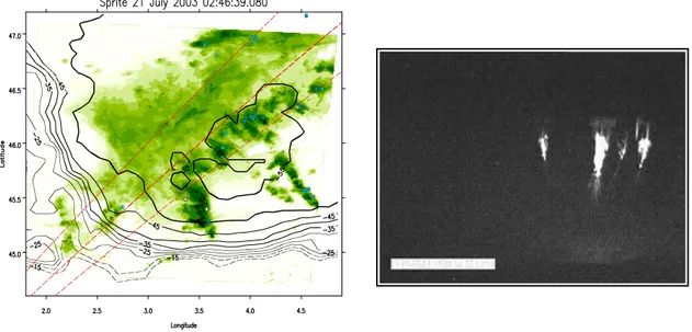
Figure 6666. Example of a carrot sprite event whose tendrils point not to the triggering +CG (the rightmost. Example of a carrot sprite event whose tendrils point not to the triggering +CG (the rightmost. Example of a carrot sprite event whose tendrils point not to the triggering +CG (the rightmost. Example of a carrot sprite event whose tendrils point not to the triggering +CG (the rightmost white +, occurring at .079 ms) but a source of charge to the west of it. Azimuths from Pic du Midi to the white +, occurring at .079 ms) but a source of charge to the west of it. Azimuths from Pic du Midi to thewhite +, occurring at .079 ms) but a source of charge to the west of it. Azimuths from Pic du Midi to the white +, occurring at .079 ms) but a source of charge to the west of it. Azimuths from Pic du Midi to the main sprite elements plotted as dashed red lines, precipitation intensity in green.
main sprite elements plotted as dashed red lines, precipitation intensity in green.main sprite elements plotted as dashed red lines, precipitation intensity in green. main sprite elements plotted as dashed red lines, precipitation intensity in green.
Sprites horizontally displaced from their causative +CG often give away a clue about its apparent source of charge removal in the cloud, by their curved appearance. Neubert et al. (2005) showed a EuroSprite 2003 example of a sprite and possible electric field lines the sprite would be aligned with. This effect should be the strongest for a point source or towards the edges of a layer source of charge. During EuroSprite, it was often observed that the tendrils of carrot sprites pointed in the direction of the +CG. But there are a number of cases where the tendrils bent towards an area significantly displaced from the triggering +CG (figure 6), even when an element itself is straight above the +CG. Thus, it appears that the region of charge removal can be tens of kilometers far from the +CG, but connected to the CG via horizontal lightning channels. This concept is worked out in chapter 5.
However, it does not explain why sprites do not always occur directly above their apparent charge removal region in the cloud, where electric fields are supposedly the highest (if the removed charge would be uniformly distributed). Frequently suggested are ion density variations in the mesosphere, with locations of enhanced ion density serving as ‘seeds’ for sprite initiation. Meteoric dust has been hypothesized to influence this (Symbalisty et al., 2000; Zabotin and Wright, 2001), as well as upward-propagating gravity waves from thunderstorms (Snively and Pasko, 2003). Sentman et al. (2003) confirmed the existance of thunderstorm-generated gravity waves in the mesosphere, but alas, sprites occurred randomly and were not found to be any brighter if superposed on a gravity wave (visible by OH-Meinel emissions), nor did they have any noticeable effect on the gravity waves. Sprites do leave ionized traces (detectable by ‘early/fast’ events in VLF radio band,
Haldoupis et al. 2004; Mika et al., 2005) which may affect subsequent sprites within the same event (Stenbaek-Nielsen et al., 2000).
Cho and Rycroft (2001) suggested that radio pulses emitted by the horizontal part of a sprite-producing lightning discharge, reflected by the ground, may create interference patterns of minima and maxima in ion density, causing preferred locations for sprite initiation. However, their calculations involved radio waves of fixed frequencies. In reality the intracloud components generate a broad spectrum of noise (Very Low Frequency sferic clusters, e.g. Johnson and Inan, 2000; Ohkubo et al., 2005; Van der Velde et al., 2006), which do not seem favorable to create organized interference patterns.
A similar hypothesis was proposed earlier by Valdivia et al. (1997), who simulated sprites developing over extensive horizontal lightning discharges. Working as fractal antennas, such discharges produce focussed areas of enhanced ion density. They found initiation is possible for charge moments as low as 100 C km, and a horizontal structure of the resulting sprite appeared very similar to reality. Neubert et al. (2005) took this as a possibility for intracloud lightning to trigger sprites on its own, but no definitely convincing evidence has so far been found. The difficulty is in proving that a CG lightning stroke really was not present. It is common for a lightning detection system to detect only 80-90% of flashes, with the inherent chance to miss the triggering stroke. One such event was discussed in Van der Velde et al. (2006), included in chapter 3. It featured intense and more complex waveforms than typical events. Furthermore, charge moment changes are based on removal of a large quantity of charge of mostly one polarity. Bidirectional development of lightning, with a negative leader propagating into positive charge and a positive leader propagating into negative charge could imply that practically equal amounts of charge of both polarities are removed from the cloud, with a resulting charge moment change that is small.
New findings reported in an article belonging to this thesis show that thunderstorm conditions and processes in lighting do influence the morphology of sprites, as explained fully in chapters 3 and 6.
Runaway electron initiation hypothesis for sprites
An alternative or perhaps co-existing candidate mechanism for sprite triggering is that of avalanches of relativistic runaway electrons (Gurevich et al., 1992) generated by lightning flashes accelerated upwards under sufficiently strong electric fields so that the energy gained from the electric field exceeds the losses from collisions. The breakdown threshold for the runaway mechanism is an order of magnitude lower and thus more easily surpassed than that of conventional breakdown: E = 218 103 N/N
0.
Runaway electrons are very energetic (~1 MeV range) and by colliding with atmospheric atoms ‘bremsstrahlung’ is created, in the form of gamma rays. The latter have first mysteriously been observed from space (Fishman et al., 1994) and are now known as Terrestrial Gamma-ray Flashes (TGF). They have been linked to thunderstorms and lightning discharges (Inan et al., 1996) and could possibly explain TLEs (Bell et al. 1995; Taranenko and Roussel-Dupré, 1996). Currently, satellite missions are planned with as
important objective to find out if TLEs are related to TGFs, such as the French TARANIS (Tool for the Analysis of RAdiations from lightNIngs and Sprites) microsatellite project, and the ASIM (Atmosphere-Space Interactions Monitor) lead by the Danish National Space Center.
The runaway breakdown mechanism might explain more easily sprite generation at the observed lower charge moment changes and lower altitudes, but encounters several difficulties, the main one being that a sprite is observed to develop also downwards after initiation, which would not be the case if triggered by runaway breakdown. Also, a small minority of sprites are reported to occur with negative CG discharges, which causes inverse electric fields and should cause any runaway breakdown to be downward-directed, thus making it impossible to produce a sprite.
However, Stolzenburg et al. (2007) found lightning flashes initiating at measured electric fields much lower than the conventional breakdown threshold, actually fitting well with the runaway breakdown threshold, surpassing it by 1.1 to 3.3 times. This may be useful at least for predicting lightning and jet initiation, although they note that surpassing the runaway threshold electric field may not be a sufficient requirement.
Negative sprites and the polarity asymmetry
While +CG flashes regulary produce sprites, only a few instances of –CG flashes have been described in literature to produce sprites. The best known is the observation by Barrington-Leigh et al. (1999) which involved large negative charge moment changes around -1600 C km. Williams et al. (2007) explored the reasons for the lack of –CG triggering of sprites (0.1% of sprites was triggered by -CG). For several continents, they calculated charge moment changes for all lightning flashes. The obtained distributions show that actually a significant part of –CGs do produce large charge moment changes typical of sprite-producing +CG flashes. So there must be a different explanation. Williams et al. (2007) suggest the impulsiveness of –CG lightning as opposed to the tendency of +CG lightning to produce continuing currents could possibly explain the asymmetry, reasoning that an electric field should exist longer in order to allow streamer development, which is not required for just the production of a halo. As described in section 2.3.2, halos are frequently observed for –CG flashes.
During EuroSprite 2006, the first confirmed negative sprite was recorded in the night of 11-12 September from Mont Aigoual over a storm over southwestern France. The triggering flash was the first -50.5 kA stroke of a three-stroked –CG according to the Météorage lightning detection network, to which the sprite was between 0-19 ms delayed. This sprite, the last one observed that night, appeared over the southern part of the stratiform precipitation region of a (at the time) poorly structured thunderstorm system that has previously only been producing sprites >30 km to the north. Within a second before this triggering –CG, also a few +CG flashes occurred in its vicinity closer to a convective core. The charge moment change of the triggering stroke has been calculated by Extremely Low Frequency radio recordings from Mitzpe Ramon in Israel and the NCK station in Hungary to be about -800 C km.
Figure Figure Figure
Figure 7777. . . . The only “negative sprite” observed during EuroSprite campaigns, caused by a -800 C km chargeThe only “negative sprite” observed during EuroSprite campaigns, caused by a -800 C km chargeThe only “negative sprite” observed during EuroSprite campaigns, caused by a -800 C km charge The only “negative sprite” observed during EuroSprite campaigns, caused by a -800 C km charge moment change –CG with a peak current of -50.5 kA.
moment change –CG with a peak current of -50.5 kA.moment change –CG with a peak current of -50.5 kA. moment change –CG with a peak current of -50.5 kA.
2.3.2 Halos
Halos are generally amorphous glows that occur at about 75 km altitude and are delayed after the initiating CG stroke by 2–6 ms, and last for a few ms (Barrington-Leigh et al., 2001; Wescott et al., 2001). They are observed together with sprites for positive CGs, but a significant fraction of haloes occurs without being accompanied by sprites. In the observations by Bering et al. (2004), halos triggered by negative CGs were more numerous than all TLEs from positive flashes, although difficult to detect visually. Thus, the halo seems to be the fundamental response to lightning. Wescott et al. (2001) showed the haloes to occur centered over the causative positive CG flash, while sprites can be displaced for the same flash. Halos are reported to occur far more often in association with negative CG flashes than sprites themselves. Moudry et al. (2003) showed an example that halos are not necessarily uniform disks, but can exhibit structure and irregular shapes. This we see confirmed also for elves observed during the night of 15-16 November 2007 over the Mediterranean, which have irregularly shaped holes.
Figure Figure Figure
Figure 8888. Four examples of halos accompanying a sprite: the diffuse disk of light on top. Halos also. Four examples of halos accompanying a sprite: the diffuse disk of light on top. Halos also. Four examples of halos accompanying a sprite: the diffuse disk of light on top. Halos also. Four examples of halos accompanying a sprite: the diffuse disk of light on top. Halos also frequently appear without sprites.
frequently appear without sprites. frequently appear without sprites. frequently appear without sprites.
2.3.3 Elves
Luminous patches of airglow near the top of the mesosphere above lightning discharges were first discovered in the Space Shuttle images by Boeck et al. (1992). During the SPRITES’95 observation campaign in Colorado, Fukunishi et al. (1996) obtained high-speed photometric data and image-intensified video showing that these events, now called elves, occur within about 160 microseconds after an intense cloud-to-ground lightning discharge at heights of 75-105 km. The observed horizontal dimensions typically range from 100-300 km, often manifesting itself as an expanding ring (Inan et al. 1997).
Elves are red-colored (but radiate also far-ultraviolet) and are brighter than sprites (1-10 MR), but last only a fraction of a millisecond which is too short to be detectable by the human eye, and also to be detected in normal video images with frame integration over >16 ms. Lightning flashes that produce elves may sometimes also produce sprites, and the reverse. The electromagnetic pulse (EMP) of the lightning return stroke is responsible for
Figure Figure Figure
Figure 9999. Examples of elves during EuroSprite2007, all occurring over the Mediterranean Sea. Some elves. Examples of elves during EuroSprite2007, all occurring over the Mediterranean Sea. Some elves. Examples of elves during EuroSprite2007, all occurring over the Mediterranean Sea. Some elves. Examples of elves during EuroSprite2007, all occurring over the Mediterranean Sea. Some elves occur together with sprites and occur at higher altitudes than the tops of those sprites. The sprite in such occur together with sprites and occur at higher altitudes than the tops of those sprites. The sprite in suchoccur together with sprites and occur at higher altitudes than the tops of those sprites. The sprite in such occur together with sprites and occur at higher altitudes than the tops of those sprites. The sprite in such cases does not necessarily occur in the middle of the hole. The top left image appears to show some gravity cases does not necessarily occur in the middle of the hole. The top left image appears to show some gravitycases does not necessarily occur in the middle of the hole. The top left image appears to show some gravity cases does not necessarily occur in the middle of the hole. The top left image appears to show some gravity waves in the elve brightness. Bottom left image shows also the associated lightning flash. The lower right waves in the elve brightness. Bottom left image shows also the associated lightning flash. The lower rightwaves in the elve brightness. Bottom left image shows also the associated lightning flash. The lower right waves in the elve brightness. Bottom left image shows also the associated lightning flash. The lower right image shows an elve with an irregular hole.
image shows an elve with an irregular hole. image shows an elve with an irregular hole. image shows an elve with an irregular hole.
creating elves by heating of electrons near the base of the ionosphere, as found remarkably consistent with measurements by Inan et al. (1997). The simulations by Veronis et al. (1999) of very short duration lightning discharges suggest that elves dominate the optical emissions for strokes <100 microseconds, while quasi-electrostatic field-generated optical emissions dominate for strokes >1 milliseconds duration.
Elves may be expected for any lightning flash with strong EMP and usually are associated with lightning peak currents greater than 50 kA, regardless of lightning polarity. Barrington-Leigh and Inan (1999), using photometers, found 100% of CGs >57 kA to produce elves, while elve brightness also increased with electromagnetic pulse strength in VLF and lightning peak current. Rakov and Tuni (2003) predicted with a transmission line model of a CG return stroke that elves may be produced for peak currents >30 kA and very fast return stroke speeds >2.5 × 10⁸ m s-1. More typically, peak currents greater than 100-120 kA are associated with elves (Huang et al., 1999). Larger peak currents have been observed by the North American Lightning Detection Network (NLDN) to occur more often over sea than over land (Lyons et al. 1998, Orville et al.,
2002), and the ISUAL instrument aboard the FORMOSAT-2 satellite has indeed observed a large majority (90%) of elves to occur over sea (Su et al., 2007).
Frey et al. (2005) noted that about half of the elves were accompanied by luminosity and VLF activity preceding that of the return stroke and elve by 2-5 ms, while the return strokes triggering sprites were not preceded by any luminosity. They suggested that a brighter, faster type of stepped leader (‘beta’) of negative ground flashes discussed in Rakov and Uman (2003) could be the cause.
Huang et al. (1999) considered it remarkable that a number of elve-producing CGs that had large enough charge moment changes to produce sprites (300 C km) failed to do so. They offer a possible explanation that elve-only discharges remove charge from smaller areas high in the storm, which gives an equal charge moment change as discharging a sheet of charge at lower altitudes, but the latter is more effective creating electrostatic fields at sprite altitudes as fields do not decrease (radially) as rapidly with height as for point charges. The higher potential of the higher source region must then explain the higher currents through the channel of the elve-producing lightning compared to that of most sprites, while the extensiveness of horizontal lightning could explain the longer delay for sprites. It must be noted that both for sprites and elves any observations of lightning structure have been very scarce or absent.
2.3.4 Jets
Characteristics
Blue jets, blue starters and gigantic jets form a family of TLE that appears to rise from high tops of certain thunderstorms and are characterized by blue and violet emissions. Blue jets and blue starters were first recorded over a storm in Arkansas during SPRITES’94 by color and black-and-white cameras observing from two airplanes (Wescott et al., 1995). These recordings remain one of the very few documented observations to date, emphasizing how rarely they are observed.
Blue jets are cones of streamers emerging from the overshooting top of the storm, moving upward with a speed of 112 ± 24 km/s, widening and fading with height, disappearing at altitudes of 37 ± 5 km (21 ± 5 km for blue starters), with durations of 200-300 ms. The cone angle varies between 6-32 degrees and the orientation varies. Wescott et al. suggested the first negative bands of N2+ are mainly responsible (391.4 nm, 427.8 nm and 470.9 nm in decreasing order of contribution) for the blue color while any red contributions are ‘quenched’ at these lower altitudes. The brightness of blue jets and starters had first been determined at 0.6 MR (Wescott et al., 1995), but with considerations of atmospheric transmission of light, Wescott et al. (1998) redetermined the brightness of these jets to higher values of 1 MR. The large Réunion island blue jet described in Wescott et al. (2001) even had a brightness of more than 6 MR.
Blue jets may occur at large rates. More than 50 blue jets were recorded in just 22 minutes, a much larger rate than is typical for sprites. The same storm produced also 30 blue starters (Wescott et al., 1996) and more than twenty upward lightning events during the same period. It was noted that the storm produced very frequent intracloud lightning flashes. While no lightning flash appeared to have directly triggered these jets, or the gigantic jet of Pasko et al. (2002) as inferred from radio sferic data, the images by Kuo et al. (2007) from the FORMOSAT-2 satellite definitely show that the cloud top delivering a gigantic jet remains lit throughout the event, though not as bright as a sprite (Steven Cummer, personal communication, 2007)
The first gigantic jet was a single event observed from Puerto Rico by Pasko et al. (2002). During the same year five events were observed also from Taiwan (Su et al., 2003), occurring in just a 20-minute time frame. Characteristic of most of the few gigantic jets reported till present (November 2007) is a leading jet rising from the cloud top to about 50-60 km with a speed of about 1000 km per second, then branching out to greater heights (70-90 km) as a tree, or a more compact luminosity like the body and hairs of carrot sprites. The upper branched part lasts about as long as a sprite. When it disappears, the lower jet remains visible while brighter parts ascend slowly along the top of the jet between 45-65 km, named the trailing jet by Su et al. (2003). The whole sequence can last as long as 200-800 ms and may feature a rebrightening. Pasko et al.’s event looks a bit different from the others in the sense that the upward speed of the leading jet could be followed by the camera, at only 100 km per second, features rebrightening, and it shows two main channels emerging from apparently one source in the cloud. It is probably due to the nanosecond gating of the image intensifier that a large amount of streamer detail is found in their images. While large ELF radio signals were detected in both cases, equal to positive downward or negative upward motions of charge, much smaller or absent ELF signals were found for the three cases studied by Van der Velde et al. (2007a, included in this work) and Van der Velde et al. (2007b).
Another class of jet-like events, named palm trees, embers or trolls (e.g. Heavner, 2000), was discovered in observations during the late 1990’s. These events are upward single or grouped jets coming from the cloud and connecting to the lower tendrils of large sprite events, their tops may branch out like a tree. According to Heavner (2000) are of red color but a detailed study by Marshall and Inan (2007) found a blue emission. In their images, the events look different than jets: they do not fan out and may actually have a broad base near the cloud. The upward speed was about 1.5 × 10⁶ m/s, quite similar to gigantic jets. The mechanism suggested by Marshall and Inan (2007) is that ionospheric electric potential can be carried along sprite bodies downward, increasing electric fields between the cloud and the sprite sufficiently to trigger the secondary, upward, event. A negative charge may be transported upward within the palm tree. Two palm tree events were recorded during EuroSprite from a thunderstorm near Mallorca, 25-26 September 2005. (Figure 10).
Figure Figure Figure
Figure 101010. Two subsequent 40 ms images of the first palm tree (troll) observed from Pic du Midi over a10. Two subsequent 40 ms images of the first palm tree (troll) observed from Pic du Midi over a. Two subsequent 40 ms images of the first palm tree (troll) observed from Pic du Midi over a . Two subsequent 40 ms images of the first palm tree (troll) observed from Pic du Midi over a Mediterranean thunderstorm, 25-26 September 2005, 1:22:04 UTC. About four upward structures can be Mediterranean thunderstorm, 25-26 September 2005, 1:22:04 UTC. About four upward structures can beMediterranean thunderstorm, 25-26 September 2005, 1:22:04 UTC. About four upward structures can be Mediterranean thunderstorm, 25-26 September 2005, 1:22:04 UTC. About four upward structures can be identified, including the bright event to the right.
identified, including the bright event to the right.identified, including the bright event to the right. identified, including the bright event to the right.
These palm trees appeared to follow a not very unusual sprite, and the left tree in the first sequence obviously grows after a sprite of only small vertical extent, so Marshall and Inan’s (2007) hypothesis may not work well here, although the sprites during this period tended to be very extensive horizontally and vertically. Altitude calculations are pending.
Figure Figure Figure
Figure 11111111. Two 40 ms images (one not shown almost eventless frame in between) of the second palm tree. Two 40 ms images (one not shown almost eventless frame in between) of the second palm tree. Two 40 ms images (one not shown almost eventless frame in between) of the second palm tree. Two 40 ms images (one not shown almost eventless frame in between) of the second palm tree (troll) observed 25-26 September 2005, 1:33:43 UTC. Clearly visible is the upward branching.
(troll) observed 25-26 September 2005, 1:33:43 UTC. Clearly visible is the upward branching.(troll) observed 25-26 September 2005, 1:33:43 UTC. Clearly visible is the upward branching. (troll) observed 25-26 September 2005, 1:33:43 UTC. Clearly visible is the upward branching.
Jet mechanisms
Cloud tops have been estimated to be as high as 18 kilometers in cases of jets. Higher tops may aid initiation by bringing charged regions into altitudes where breakdown and streamer corona propagation thresholds are lower. The first theoretical models based on the conventional air breakdown mechanism, by Pasko et al. (1996) and Sukhorukov et al. (1996), suggested blue jets were large positive or negative streamers (waves of ionization) moving upward under the influence of the vertical electric field. They required discharging of the lower charge center or rapid charge accumulation to initiate the jet as result of a threshold electric field. Later modelling efforts (Pasko and George, 2002) supposed that jets consist of narrow fractal streamers. The jet continues to move upward as long as a minimum local electric field requirement is met. Multiple-streamer structure at the sides of jets was observed first in the Réunion island photograph studied by Wescott et al. (2001), which contained eight side branches from a main channel, as well as the gigantic jet by Pasko et al. (2002), and was predicted by Petrov and Petrova (1999). In
Pasko and George’s work, the maximum height of the modelled event depends on the charge supplied by the storm cloud. Raizer et al. (2006, 2007) addressed the shortcomings of the fractal model. The charge inside the cloud must be gathered from the hydrometeors and supplied to the jet by conducting hot leaders, as opposed to cold streamers that are non-conducting at the time scale of the jet, so it is likely that a bi-leader process as in common lightning is involved. This has the advantage that less charge is needed because the leader channel carries the potential of the source region out of the cloud, providing high electric fields at the tip. The streamers that run ahead of the leader tip are still dependent on the existance of a minimum required field for their propagation.
Krehbiel et al. (2008) detected a blue jet in the data of the New Mexico Lightning Mapping Array. They suggest that the presence of screening layer charge at edges of electrified clouds, a requirement also for initiation of downward cloud-to-ground lightning (e.g. Mansell et al., 2002), is likely required as well for allowing outward growth of jets by increasing local fields.
Observational aspects
The observation of blue events is more difficult than red events, which is probably the reason that they are not observed more frequently. As Rayleigh scattering is inversely proportional to wavelength as λ-4, the light of a blue-violet event (near 400 nm) event will be extincted at least ten times more with distance compared to a near-infrared event (700 nm), which decreases the odds that jets can be seen from long distances and low altitudes. Additionally, the cameras typically used are less sensitive for violet light (40-50% response at 390 nm) than for near-infrared light emitted by sprites (still 80% response near 700 nm). Together this means if a sprite appears as bright as a star with a visual magnitude of +3 at a typical observing distance of 300 km, a typical blue jet emitting light twice as bright as the sprite at the same distance should appear about 2.5 magnitudes dimmer (2.5122.5 equals a factor of 10). For jets to appear as clearly in unintensified images as sprites with these cameras, typical observing distances need to be much closer than for sprites, preferably within 150 kilometers.