Error estimation of a proper orthogonal decomposition reduced model of a permanent magnet synchronous machine

Science Arts & Métiers (SAM)

is an open access repository that collects the work of Arts et Métiers Institute of Technology researchers and makes it freely available over the web where possible.

This is an author-deposited version published in: https://sam.ensam.eu

Handle ID: .http://hdl.handle.net/10985/9264

To cite this version :

Thomas HENNERON, Hung MAC, Stéphane CLENET - Error estimation of a proper orthogonal decomposition reduced model of a permanent magnet synchronous machine - In: Computation in Electromagnetics (CEM 2014), 9th IET International Conference on, United Kingdom, 201403 -Computation in Electromagnetics (CEM 2014), 9th IET International Conference on - 2015

Error Estimation of a POD Reduced Model of a Permanent Magnet

Synchronous Machine

T. Henneron1, H. Mac2, S. Clénet2

1

L2EP, University of Lille1, Lille, France, thomas.henneron@univ-lille1.fr

2

L2EP, Arts et Métiers ParisTech, Lille, France, stephane.clenet@ensam.eu

Keywords: Model order reduction, Proper Orthogonal Decomposition, Error estimation, electrical

machine.

Abstract

Model Order Reduction Methods, like the Proper Orthogonal Decomposition (POD), enable to reduce dramatically the size of a FE model. The price to pay is a loss of accuracy compared to the original FE model that should be of course controlled. In this paper, we apply an error estimator based on the verification of the constitutive relationship to compare the reduced model accuracy with the full model accuracy when POD is applied. This estimator is tested on an example: a permanent magnet synchronous machine.

1 Introduction

To study electrical devices with the help of numerical approach, the Finite Element Method combined with a time-stepping scheme is often used. The computation time of the large system of equations obtained from the discretization of the Maxwell equations can be prohibitive with a fine mesh and a small time step is applied. To decrease the computation time, Model Order Reduction (MOR) methods can be an alternative since they enable to create a model of small size from a complete Finite Element (FE) model. The price to pay is a loss of accuracy compared to the original FE model. In the literature, the Proper Orthogonal Decomposition is one of the most popular MOR methods to solve problems in engineering [1]. The POD consists in performing a projection of the solution of the original model (FE model for example) onto a reduced basis, yielding a reduction of the size of the equation system. The snapshot approach is often used to determine the discrete projection operator between the original basis (generated from the mesh in the case of a FE model) and the reduced basis [2]. For example, when solving a FE model in the time domain, the idea is to evaluate the solution of the original model for the

first time steps (the snapshots) and then to extract from these snapshots the projection operator. Then, the reduced model is solved for the other remaining time steps. In computational electromagnetics, the POD method combined with the snapshot technique has been developed in order to study linear and non-linear problems or magnetostatic and quasistatic problems [3-7]. In the case of a rotating electrical machine, the snapshots correspond to the solution of the original model for different positions of the rotor [8,9]. The accuracy of the POD method depends on the number and also on the distribution of the snapshots on the whole interval of rotation. This aspect has been emphasised in [9] where the influence of the snapshot distribution on the accuracy of the reduced model in the case of a rotating permanent magnet synchronous machine has been clearly shown. Therefore, when applying the POD, an error estimator can be very useful not only to control the loss of accuracy versus the original FE model, but also to optimize the distribution of the snapshots.

In this paper, an error estimator based on the verification of the magnetic constitutive relationship is developed in magnetostatics when POD is applied. This estimator enables to evaluate the distance between the numerical solution (obtained from the original or the full model) and the exact solution without knowing it [10,11]. This estimator is then used to compare different snapshot distributions in terms of accuracy. In the first part, the error estimator is developed for a magnetostatic problem. In a second part, the reduced numerical model obtained from the snapshot POD approach is presented. Finally, a permanent magnet synchronous machine is studied to illustrate the proposed approach. Different distributions of the snapshots will be studied and compared using the proposed error estimator.

2 Error estimation

2-1 Magnetostatic Problem

Let consider a couple (H,B) verifying the two equilibrium equations in magnetostatics on a domain D and the conditions on the boundary Γ (Γ=Γh∪Γb and 0=Γh∩Γb) that is to say:

curl H = J and nxH=0 on Γh

div B = 0 and n.B=0 on ΓB

(1.a) (1.b)

with J the current density and n the outward unit vector. The behaviour of the material is assumed to be linear and we denote by µ the permeability. If the couple (H,B) verifies the behaviour law B=µH on D

then it is equal to the exact solution (Hex,Bex) of the magnetostatic problem. We consider now the term ε such that:

2 2 1 − µ µ − = ε B H (2) with _µ− =

_∫

-norm since the permeability µ is a strictly positive function. Then, it can be shown that [10]: 2 2 2 µ µ + − − = ε B Bex −1 H Hex (3)

The relationship (3) shows that the scalar ε is equal the sum of the two terms representing the distances either between B and Bex or H and Hex. If ε is equal to zero then the couple (H,B) is equal to the exact

solution (Hex,Bex). If ε is not equal to zero, ε is an error estimator because it is a bound of the distance between the admissible field and the exact solution (3).

In practice, this error estimator is commonly used to evaluate the discrepancy error introduced by the discretisation of space when applying the Finite Element Method. The admissible couple (H,B) is calculated from the solution of the dual formulations in magnetostatics [10]. In the case of the vector potential formulation, from (1.a), the magnetic flux density B is expressed such as B = curl A with A the vector potential and nxA=0 on Γb with. Then, according to (1.b), in the case of the vector potential

formulation, the following equation is solved:

curl (µ−1curl A) = J (4)

In the case of the scalar potential formulation, from (1.b), the magnetic field H is expressed such as H =

Hs - grad Ω with Ω the scalar potential, curl Hs = J, nxHs=0 on Γh and Ω = cte on Γh. Then, according

to (1.a), in the case of the scalar potential formulation, the following equation is solved:

div (µ (ΗΗΗΗs −grad Ω)) = 0 (5)

The solution of the scalar (resp. vector) potential formulation gives a magnetic field H (resp. a magnetic flux density B) verifying (1.a) (resp. (1.b)). Then, from the couple (H,B) obtained by solving both potential formulations, the error is estimated by calculating the scalar ε using (2).

2-2 FE Model for an electrical machine

We assume that the domain D is divided into two parts: the static part and the moving part. In the following, we consider only rotation but the method can be also applied for translation or for a combination of both. We denote by an angle θ the angular position of the moving part with respect to the static part. Then, the magnetic field distribution depends on the angle θ. Neglecting the eddy currents, the modelling of the electrical machine considered in the following is based on the magnetostatic formulation (see section 2.1) and is solved using the Finite Element Method. The movement is taken into account using the locked step technique. The angular positions θi (1≤i≤N) are then equally distributed in the

interval [0,2π]. At each angular position θ=θi (1≤i≤N), both potential formulations are solved. For each

formulation, the following linear equation system is [8]:

M(θ) X(θ)=F(θ) (6)

with M(θ) the stiffness matrix, F(θ) the source vector and X(θ) the vector of the Degrees of Freedom (DoFs). The number of DoFs is denoted by n. The DoFs in the scalar potential formation are the values of the scalar potential Ω at the nodes of the mesh. The magnetic field Hi obtained from the scalar potential

formulation at θ=θi verifies (1.a). In the vector potential formulation, the DoFs are the circulations of the

potential A along the edges. The magnetic flux density Bi obtained by the vector potential formulation at

θ=θi verifies (1.b). For any angular position θ, it is straightforward to extrapolate a couple (H(θ),B(θ))

verifying (1.a) and (1.b) for any position θ∈[θi,θi+1] as:

( )

(

)

( )

(

)

By applying (2), we can obtain an estimation of the error εFEM(θ) in function of the position θ due to the

3 Model Order Reduction

In order to reduce the computation time required to solve (6), the Proper Orthogonal Decomposition method is used [1][2]. The vector X(θ) is approximated in a reduced basis by using a vector Xr(θ) of size

Ns (Ns<<n) and a discrete projection operator ΨΨΨΨ such that:

X(θ) ≈ΨΨΨΨ Xr(θ) (8)

To construct the operator ΨΨΨΨ, the snapshot approach is typically used [2]. The full problem (6) is solved

for Ns angular positions θi. The Ns solutions are so-called snapshots. We denote by S the 1xNs vector of

position indices of the snapshots (i=Sj is the index the position θi of the jth snapshot). Then, a snapshot

matrix Ms is built from these Ns snapshots such that Ms=(Xj)1≤j≤Ns with Xj the solution X(θi) and i the jth

entry of the vector S. Applying a Singular Value Decomposition, the matrix Ms can be decomposed under

the form:

∑

with Vn×n and WNs×Ns orthogonal matrices and ΣΣΣΣn×Ns the diagonal matrix of the singular values Σi. The ith

row of W corresponds to the components of the ith vector of the matrix Ms projected in the reduced basis

formed by the Ns vectors of the matrix VΣΣΣΣ. Then, the operator ΨΨΨΨ is a selection of r vectors of the matrix V

corresponding to the singular values Σi higher than a given threshold (fixed arbitrarily). Finally, by

combining (6) and (8), the reduced model to be solved can be written as:

Mr(θ) Xr(θ)=Fr(θ) (10)

with Mr(θ)=tΨΨΨΨM(θ)ΨΨΨΨ and Fr(θ)=tΨΨΨΨF(θ). The size of the equation system (10) is rather small compared to

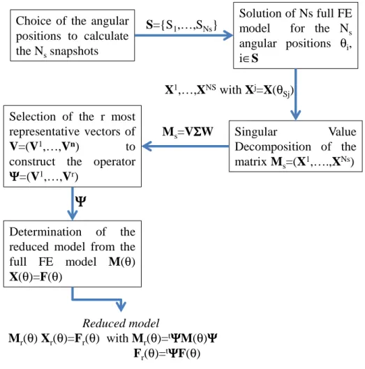
(6) since r<<n. In Figure 1, we give a flow chart gathering all the different steps of the snapshot POD, described above.

The system (10) is solved for each angular position θ=θi giving a solution Xr(θi), then by applying (8) an

posed since the discrepancy comes not only from the FE discretisation but also from the process of reduction. The solution of the reduced problem using both potential formulations at each time step enables to calculate a couple (H’(θ),B’(θ)) verifying (1.a) and (1.b) for any angular position θ (see (5)). Then an error εMOR(θ) can be defined calculating (3) for each position. A global error εMOR,GLO can be

also defined by integrating εMOR(θ) over a period.

Choice of the angular positions to calculate the N_ssnapshots

Solution of Ns full FE

model for the N_s

angular positions θ_i, i∈S

Singular Value

Decomposition of the matrix M_s=(X1_,….,XNs₎ Selection of the r most

representative vectors of

V=(V1_,…,Vn_{) to}

construct the operator

Ψ Ψ Ψ

Ψ=(V1_,…,Vr₎

Determination of the

reduced model from the

full FE model M(θ) X(θ)=F(θ) Reduced model M_r(θ) X_r(θ)=F_r(θ) with M_r(θ)=tΨΨΨΨ_M(θ₎ΨΨΨΨ F_r(θ)=tΨΨΨΨ_F(θ₎ S={S₁,…,S_Ns} X1_,…,XNS_{with X}j_=X(θ Sj) M_s=VΣΣΣΣW

Ψ

Ψ

Ψ

Ψ

Figure 1: Flow chart describing the process to obtain the reduced model from the full FE model by applying snapshot POD

5 Application

The 8-pole permanent magnet synchronous machine studied at no load operation is presented in Figure 2. The full FE model with 40449 nodes and 53672 prisms has been solved for 180 angular positions

θ∈[0,90°] (the angle step is equal to 0.5 degree). The aim of the study is to analyse the error related to the choice of the snapshots. Three configurations for the construction of the reduced basis are considered. For the first configuration, the reduced basis is determined from Ns snapshots corresponding to the first Ns

angular positions. For the second configuration, the reduced basis is determined from Ns snapshots uniformly distributed in [0,90°] that is to say that the angular position of the snapshots are θj =90(j-1)/Ns

with j∈[1,Ns]. For the last configuration, we consider all positions considered in the FE model as

snapshots but only the r first vectors of VΣΣΣΣ are considered to construct the projection matrix ΨΨΨΨ.

The last configuration has no practical interest because it requires the solution of the full FE model for all angular positions. This configuration, however, leads to the best reduced basis for a given NS. In the

following, the last configuration will be considered as a reference enabling to evaluate the accuracy of the two first configurations which are practically relevant because they only require the solution of the full problem for Ns positions (Ns<<N).

Figure 2: Permanent magnet machine

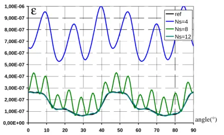
Figures 3, 4 and 5 give the errors εFEM(θ) of the reference model (i.e. full model) and the errors εMOR(θ)

for different values of Ns and for the three configurations. For all configurations, the error of the reduced model decreases with the number of snapshots. For the first configuration where the snapshots correspond to the first time steps, the error εMOR(θ) is equal to εFEM(θ) obtained from the full model for these angular

positions. But for θ greater than Ns*90/N, εMOR(θ) differ significantly from εFEM(θ). For the second

configuration, we notice that the error given from the reduced model are the same as the one of the reference model for the snapshots used to determine the reduced model (θj =(j-1)*90/Ns with j∈[1,Ns]).

The maximum of the error is located at the center between two successive snapshots and this maximum value decreases with an increasing number of snapshots. For the last configuration, the error obtained from the reduced model is close to the reference for Ns=12.

0,00E+00 5,00E-06 1,00E-05 1,50E-05 2,00E-05 2,50E-05 3,00E-05 0 10 20 30 40 50 60 70 80 90 ref Ns=5 Ns=10 Ns=20 Ns=30

ε

Figure 3: Evolution of the error estimation for the first configuration 0,00E+00 5,00E-07 1,00E-06 1,50E-06 2,00E-06 2,50E-06 3,00E-06 3,50E-06 4,00E-06 0 10 20 30 40 50 60 70 80 90 ref Ns=4 Ns=8 Ns=12

ε

Figure 4: Evolution of the error estimation for the second configuration 0,00E+00 1,00E-07 2,00E-07 3,00E-07 4,00E-07 5,00E-07 6,00E-07 7,00E-07 8,00E-07 9,00E-07 1,00E-06 0 10 20 30 40 50 60 70 80 90 ref Ns=4 Ns=8 Ns=12

ε

Figure 5: Evolution of the error estimation for the third configuration

We denote by εMOR,GLO and εFEM,GLO the global error obtained from the reduced and reference models.

Figure 6 presents the ratio |εFEM,GLO-εMOR,GLO|/ εMOR,GLO as a function of the number of snapshots for all

configurations. In order to compare the error on the magnetic field, an error estimation based on the magnetic flux linked to the first stator winding is defined. For all positions of the rotor, the L2-norm of the difference of the magnetic flux linkage obtained from the two formulations is computed by ∆Φ=|ΦA

-ΦΩ|2 with ΦA and ΦΩ the vectors of the magnetic flux linkage for all positions obtained from the vector

and scalar formulations. Figure 7 shows the ratio |∆ΦFEM-∆Φ MOR|/∆ΦFEM as a function of the number of

snapshots for all configurations. For both error estimators, the dependences of the error on the number of snapshots are similar meaning that the error estimator ε represents correctly the discrepancy on the magnetic flux linkage even after reduction. The errors decrease when the number of snapshots increases.

With the first configuration, the error decreases slowly compared to the others ones. For the second and the third configurations, the shapes of the errors are similar: the error obtained from the third configuration is smaller than the one associated with the second configuration when the number of snapshots is larger than 2. As explained before, the error of the third configuration can be considered as the reference error of the reduced model. With the second configuration, it is possible to obtain errors close to those of the third configurations when the Ns snapshots are uniformly distributed in [0,90°]. In order to compare the reduced basis generated from the second and third configuration, Figures 8 and 9 show the distributions of curl ΨΨΨΨi for i={1,4} obtained from the vector potential formulation. The

distributions are similar for the three first vectors and a difference firstly appears for the fourth vector. Physically, the distribution of curl ΨΨΨΨ1 can be interpreted as a homopolar field component. The

distributions of curl ΨΨΨΨ2 and curl ΨΨΨΨ3 are similar but shifted with an electrical angle of π/2. They can be

interpreted as longitudinal and transverse field distributions of the magnetic field density.

0 20 40 60 80 100 120 0 5 10 15 20 25 30 1-conf 2-conf 3-conf Ns %

Figure 6: Evolution of the error estimation |εFEM,GLO-εMOR,GLO|/ εMOR,GLO (%)

0 5 10 15 20 25 30 35 40 45 50 0 5 10 15 20 25 30 1-conf 2-conf 3-conf Ns %

Figure 7: Evolution of the error

|∆ΦFEM-∆Φ MOR|/∆ΦFEM (%) of the magnetic flux

Figure 8: Distributions of curl ΨΨΨΨi for i={1,4} obtained from the second configuration

Figure 9: Distributions of curl ΨΨΨΨi for i={1,4} obtained from the third configuration

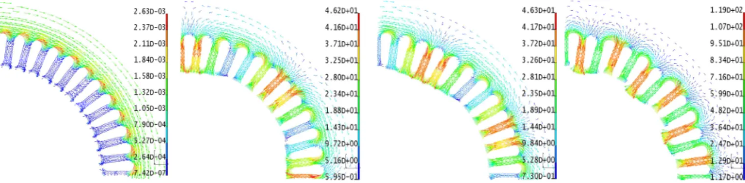
In order to evaluate the magnetic flux linkage obtained from the second and third configurations, Figures 10 and 11 show the magnetic flux linkage deduced from the vector potential formulation for different numbers of snapshots and for both configurations. The magnetic flux linkage are similar nevertheless, as shown in Figure 8, the result obtained from the third configuration converges toward the reference faster than the one of the reduced model. In order to obtain an acceptable shape, the reduced model deduced from the third configuration requires 8 vectors in the reduced basis whereas for the second configuration, 16 vectors are necessary. Figure 12 presents the distribution of the magnetic flux density obtained from the reference configuration and the difference of the distribution between the reference and this from the second and third configurations. The number of snapshots is 16 for the second configuration and 12 for the third configurations in order to keep the same range of the error. We can see that the maximum difference is not located where the magnetic flux density is maximum.

-0,055 -0,035 -0,015 0,005 0,025 0,045 0 10 20 30 40 50 60 70 80 90 ref Ns=2 Ns=4 Ns=8 Ns=12 Ns=16 Φ(Wb) angle(°)

Figure 10: Evolution of the magnetic flux linkage linked with the first winding obtained from the vector formulation and the second configuration

-0,055 -0,035 -0,015 0,005 0,025 0,045 0 10 20 30 40 50 60 70 80 90 ref Ns=2 Ns=4 Ns=8 Φ(Wb) angle(°)

Figure 11: Evolution of the magnetic flux linkage linked with the first winding obtained from the

vector formulation and the third configuration

Figure 12: Distribution of the magnetic field density (T) in the stator obtained from the vector potential formulation and the difference of the distribution between the reference and this from the second and third configurations (reference, second configuration with Ns=16 and third configuration with Ns=12)

6 Conclusion

In this paper, an error estimator based on the discrepancy of the constitutive relationship has been introduced in order in evaluate the quality of a reduced model obtained from the snapshot POD method. This error estimator has been applied successfully to compare different snapshot distributions for a rotating permanent magnet synchronous machine. It has been found that a uniform distribution of the snapshots is almost optimal and enables to get results which are very close to the original model but only with a dozen of snapshots. The error estimator can be very useful in numerous other applications. For

example, it can be applied to determine adaptively the snapshot distribution. Indeed, according to a given distribution of snapshots, the error in function of the position can be estimated. For the positions where the error is the highest, the full problem can be solved to enrich the set of snapshots. The error estimator can be used to compare different MOR methods like snapshot POD, PGD or other reduction methods in the case of rotating electrical machines.

Acknowledgements

This work is supported by the IAP7/M2E2S (Belgium state) and MEDEE pole supported by the region council of Nord Pas de Calais (France) and the European Community.

References

[1] Lumley J., Yaglom, A.M., Tatarski, V.I.:“The structure of inhomogeneous turbulence”, Atmospheric Turbulence and Wave Propagation, 1967, pp. 221–227

[2] Sirovich, L.: “Turbulence and the dynamics of coherent structures”, Q. Appl. Math., XLV (3), 1987, pp. 561–590

[3] Zhai, Y.:“Analysis of Power Magnetic Components With Nonlinear Static Hysteresis: Proper Orthogonal Decomposition and Model Reduction”, IEEE Trans. Mag., 2007, 43(5), pp. 1888-1897 [4] Schmidthäusler, D., Clemens, M.: “Low-Order Electroquasistatic Field Simulations Based on Proper

Orthogonal Decomposition”, IEEE Trans. Mag., 2012, 48(2), pp. 567-570

[5] T. Henneron, S. Clénet, “Model Order Reduction of Non-Linear Magnetostatic Problems Based on POD and DEI Methods”, IEEE Trans. Mag., 2014, 50(2)

[6] Rutenkroger, M., Deken, B., Pekarek, S.:“Reduction of model dimension in nonlinear finite element approximations of electromagnetic systems”, in Proc. IEEE Workshop Computers in Power Electronics, 2004, pp. 20–27

[7] Sato, Y., Igarashi, H.:“Model Reduction of Three-Dimensional Eddy Current Problems Based on the Method of Snapshots”, IEEE Trans. Mag, 2013, 49(5), pp. 1697-1700

[8] Albunni, M.N., Rischmuller, V., Fritzsche, T., Lohmann, B.:“Model-Order Reduction of Moving Nonlinear Electromagnetic Devices”, IEEE Trans. Mag., 2008, 44(7), pp. 1822-1829

[9] Henneron, T., Clénet, S.:“Model order reduction applied to the numerical study of electrical motor based on POD method“, International Journal of Numerical Modelling: Electronic Networks, Devices and Fields, 2014, 27(3), pp. 485-494

[10] Prager, W., Synge, J.L.:“Approximation in elasticity based on the concept of functions space”, Quart. Appl. Math., 5, 1947, pp 261-269

[11] Marmin, F., Clénet, S., Piriou, F., Bussy P., “Error Estimation of finite element solution in non linear magnetostatic 2D problems», IEEE Trans. Mag., 1998, 34(5), pp 3268-3271

[12] Sadowski N., Lefevre Y., Lajoie-Mazenc M., Cros J., “Finite element torque calculation in electrical machines while considering the movement”, IEEE Trans. Mag., 1992, 28(2), pp. 1410-1413

[13] Arkkio A., “Finite element analysis of cage induction motors fed by static frequency converters”, IEEE Trans. Mag., 1990, 26(2), pp. 551–554