Sciences de l'Univers, de l'Environnement et de l'Espace (SDU2E)
Etude diagnostique de la variabilité de la salinité de surface de l'Océan
Pacifique. Apport des données SMOS.
15 Octobre 2013
Audrey HASSON
Océanographie PhysiqueM. Gilles REVERDIN, Rapporteur, LOCEAN M. Jerome VIALARD, Rapporteur, LOCEAN
Thierry Delcroix UMR5566 LEGOS
Mme Jacqueline BOUTIN, Examinateur, LOCEAN M. Thierry DELCROIX, Directeur de thèse, LEGOS
M. Jordi FONT, Examinateur, Institut de Ciències del Mar CMIMA-CSIC Mme Fabienne GAILLARD, Examinateur, LPO Ifremer
La salinité est un paramètre clé de l’océan car elle impacte la dynamique océanique par la densité. Elle est considérée comme une Variable Climatique Essentielle. La distribution du sel dans l’océan est le résultat d’un équilibre subtile entre le forçage de surface (Evaporation moins Précipitation), l’advection horizontale de sel (aux basses et hautes fréquences) et le forçage vertical de sub-surface (entrainement et mélange), chacun de ces termes étant d’égale importance. Même si ces processus sont bien connus de façon qualitative, quantifier l’effet de chacun d’entres eux est un challenge et toujours une question ouverte. Mon travail de thèse a pour but de : a) quantifier les mécanismes responsables de la variabilité de la salinité de surface dans l’Océan Pacifique tropical (principalement aux échelles saisonnières et interannuelles), b) décrire et évaluer les processus à l’origine des variations de salinité de surface pendant l’évènement La Nina de 2010-2011 et c) analyser la formation et la variabilité du noyau de maximum de sel de l’Océan Pacifique subtropical (aux mêmes échelles de temps). Pour se faire, différents jeux de données sont utilisés conjointement : des observations de salinité in situ principalement des bateaux marchands et des profileurs Argo, des données de salinité de surface dérivées du nouveau satellite SMOS ainsi que d’autres produits issus de mesures satellitaires tels que les précipitations, l’évaporation et les courants de surface. Une simulation spécifique d’un modèle forcé est aussi employée. Les principaux résultats de ce travail sont publiés, « in press » et soumis dans des journaux à comités de lecture.
Salinity is one of the key parameters of the ocean impacting its dynamics through density. It is considered as an Essential Climate Variable. The salinity patterns result from a subtle balance between surface forcing (E-P, Evaporation minus Precipitation), horizontal salt advection (at low and high frequencies) and subsurface forcing (entrainment and mixing), all terms being of analogous importance. While processes responsible for sea surface salinity (SSS) changes are qualitatively well known, quantifying those mechanisms is very challenging and hence still under debate. My Ph.D. research work aims at: a) quantifying mechanisms responsible for the tropical Pacific Ocean SSS variability (mainly at seasonal and ENSO time scale), b) describing and assessing mechanisms behind the 2010-2011 La Niña SSS changes, and c) analysing the formation and variability of the south Pacific subtropical high SSS core (at the same time scales). In order to do so, various datasets are used conjointly: in-situ salinity observations mainly from voluntary observing ships and Argo profilers, satellite based surface salinity (from SMOS), precipitation, evaporation and near-surface currents as well as a specific forced model simulation. The main results of my work are published, in press and submitted in peer review research articles.
RESUME 1
ABSTRACT 2
TABLE OF CONTENTS 3
CHAPTER 1. INTRODUCTION 7
I. SALINITY 7
I.1. STANDARD DEFINITION 7
I.2. PRACTICAL DEFINITIONS 8
I.3. SALINITY GEOLOGICAL CYCLE 11
II. IMPORTANCE OF SALINITY IN OCEANOGRAPHY 13 II.1. A PROXY TO TRACK WATER MASSES 13
II.2. A MARKER FOR FRONTAL REGIONS 14
II.3. A TOOL TO ESTIMATE THE FRESHWATER CYCLE 15
II.4. THE SEAWATER EQUATION OF STATE 17
II.5. ROLE ON DEEP WATERS FORMATION (HIGH LATITUDES) 19
II.6. ROLE ON MIXED LAYER VIA BARRIER LAYER FORMATION (LOW LATITUDES) 20
II.7. SALINITY ASSIMILATION AND IMPACT ON ENSO PREDICTION 22
III. IN SITU S DATA PROGRAMS 23
IV. DESCRIPTION OF SSS PATTERNS – MEAN STATE 25
IV.1. MEAN SSS IN THE GLOBAL OCEAN 25
IV.2. MEAN SSS IN THE TROPICAL PACIFIC OCEAN 28 V. SSS VARIABILITY IN THE TROPICAL PACIFIC OCEAN– A BRIEF LITERATURE REVIEW 29
V.1. SMALL TIME/SPACE SCALES 29
V.2. INTRASEASONAL TIME SCALES 30
V.3. SEASONAL VARIABILITY 32
V.4. INTERANNUAL VARIABILITY 34
V.5. DECADAL VARIABILITY 37
V.6. CLIMATE SHIFTS 39
V.7. TENDENCY IN RECENT DECADES 39
V.8. PROJECTED SSS CHANGES UNDER GLOBAL WARMING 41
I. DATA DESCRIPTION 45
I.1. IN-‐SITU OBSERVATIONS 45
I.1.1. VOS Bucket samples and TSG 45
I.1.2. Other Salinity Observations 46
I.2. GRIDDED PRODUCTS 49
I.2.1. The tropical Pacific SSS Product 49
I.2.2. ISAS 50
I.3. SMOS 51
I.4. MODEL SIMULATION MRD911 54
I.5. ADDITIONAL DATASETS 56
I.5.1. Near-‐surface currents 56
I.5.2. Precipitations 56
I.5.3. Evaporation 56
I.5.4. Mixed Layer Depth 56
II. METHODOLOGY 57
II.1. MIXED LAYER SALINITY (MLS) BUDGET 57
II.2. SIGNAL PROCESSING 58
II.2.1. Mean seasonal signal 58
II.2.2. Interannual signal 59
II.3. COMPUTING PROCEDURES 59
CHAPTER 3. THE MIXED LAYER SALINITY BUDGET IN THE TROPICAL PACIFIC OCEAN 61
FOREWORD 61
ARTICLE 61
ABSTRACT 62
I. INTRODUCTION 62
II. METHODOLOGY, DATA AND MODEL DESCRIPTION 65
II.1. METHODOLOGY 65
II.2. OBSERVATIONAL DATA 65
II.3. MODEL DATA 65
II.4. MODEL ASSESSMENT 66
III. MIXED-‐LAYER SALINITY BUDGET 66
III.1. MEAN STATE 67
III.2. SEASONAL TIME SCALE 70
IV.1. THE 1997-‐1998 EASTERN PACIFIC EL NINO 73
IV.2. THE 2002-‐2003 CENTRAL PACIFIC EL NINO 74
V. CONCLUSION 75
AKNOWLEDGEMENTS 76
REFERENCES 76
CHAPTER 4. ANALYSING THE 2010-‐2011 LA NIÑA SIGNATURE IN THE TROPICAL PACIFIC SEA SURFACE SALINITY USING IN SITU, SMOS OBSERVATIONS AND A NUMERICAL
SIMULATION 79
FOREWORD 79
ARTICLE 79
ABSTRACT 79
I. INTRODUCTION 80
II. DATA AND METHODS 83
II.1. DATA DESCRIPTION 83
II.2. DATA ASSESSMENT 85
III. THE 2010-‐2011 ENSO SIGNATURE IN SSS 88 IV. MECHANISMS ASSOCIATED WITH THE 2010-‐2011 SSS ANOMALIES 91
V. COMPARISON WITH THE 1998-‐1999 LA NIÑA 94
VI. SUMMARY AND CONCLUSION 97
AKNOWLEDGEMENTS 99
REFERENCES 99
CHAPTER 5. FORMATION AND VARIABILITY OF THE SOUTH PACIFIC SEA SURFACE
SALINITY MAXIMUM IN RECENT DECADES 101
FOREWORD 101
ARTICLE 101
ABSTRACT 101
I. INTRODUCTION 102
II. DATA DESCRIPTION AND ASSESSMENT 104
III. CAUSES OF THE HIGH-‐SALINITY CORE FORMATION 106
IV. VARIABILITY OF THE HIGH-‐SALINITY CORE 108
IV.1. SEASONAL VARIABILITY 108
IV.2. INTERANNUAL VARIABILITY 112
REFERENCES 117
CHAPTER 6. CONCLUSIONS AND PERSPECTIVES 119
I. CONCLUSIONS 119
II. PERSPECTIVES 125
II.1. TECHNICAL ISSUES 125
II.2. SCIENTIFIC PERSPECTIVES 127
II.2.1. Formation of the South Pacific SSS maximum 127
II.2.2. TIW and surface salinity budget 127
II.2.3. The Barrier Layer and ENSO 128
II.2.4. Trend in salinity 129
II.3. INFERRING THE MARINE FRESH WATER CYCLE 130
Chapter 1. Introduction
The three key physical variables in the ocean are its temperature, salinity and pressure, which are linked together by density via the seawater equation of state (e.g., see, Gill, 1982; Millero, 2010). Density is of particular importance since small spatial gradients can drive the ocean circulation, which redistributes heat meridionally and therefore contributes to the global climate system. Historically, studies of the ocean temperature have been abundant because of the relative high numbers of in situ temperature profiles and remotely-sensed surface measurements and its major influence on density. In contrast, the role of salinity in the ocean remains under-explored, mainly because of the lack of data.
The present thesis analyses salinity mean patterns in the tropical Pacific Ocean and their temporal and spatial variability. In the following introductory Chapter, the reader will be first introduced to the different evolving definitions of salinity (Section I), then to the importance of salinity in oceanography (Section II). We will subsequently describe the in situ salinity data presently available to scientists (Section III). A description of the mean SSS in the Global Ocean and in particular in the tropical Pacific Ocean will be given (Section IV) as well as a brief literature review of its variability at different time/space scales (Section V). Finally, we will underline three major issues insufficiently addressed in literature (Section VI), which will be the base of this thesis.
I. Salinity
Our knowledge of salinity has been growing since the late 19th
century and its definition has evolved in parallel. This complex evolution, detailed in Millero et al. (2008) and the references therein, is briefly described in this section. In the first sub-section, we will present the conceptual definition of salinity, followed by the evolution of salinity measurements leading to practical definitions. The last sub-section will focus on the salinity geological cycle, which explains the salt contents of seawater.
I.1. Standard Definition
Salinity is the "Total amount of dissolved material in grams in one kilogram of sea water" (Sverdrup et al, 1942). Salinity is therefore the ratio of the weight of drought matter
over the weight of water sample. Salinity is dimensionless and has consequently no unit but a scale: the practical salinity scale (pss) corresponding to g/kg. Salinity was first measured in the 19th
century by weighing what was left after complete evaporation. However, this method was highly inaccurate as some components were lost during the process.
The Principle of Constant Proportions states that “regardless of the absolute
concentration, the relative proportions of the different major constituents are virtually constant”(Dittmar, 1884), except in regions of high dilution (low salinity), where minor
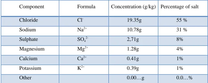
deviations may occur. Table 1 presents the average composition of these major constituents in 1 litre of seawater with a salinity of 35.000 pss. The different constituents’ concentrations for lower or higher salinity can be obtained by scaling by the same factor. From this table, we note that chloride and sodium are the principal constituents of the dissolved matter in seawater, respectively accounting for 55 and 31%, and are the main component of what is commonly called “table salt”.
Component Formula Concentration (g/kg) Percentage of salt
Chloride Cl- 19.35g 55 % Sodium Na2+ 10.78g 31 % Sulphate SO4 2- 2,71g 8% Magnesium Mg2+ 1.28g 4% Calcium Ca2+ 0.41g 1% Potassium K2+ 0.39g 1% Other 0.00…g 0.0…%
Table I.1 Salt composition of an average sample of one litre of seawater with SP=35.000 pss (Pawlowicz, 2013)
I.2. Practical Definitions
Because of the (quasi) unvarying composition of salt ions in seawater, salinity can theoretically be deduced by measuring one of them and using a simple scaling. Chloride, one of the dominant components, can be measured by a simple chemical analysis. Using Copenhagen “Normal water” standards, Salinity is defined by Knudsen (1903) based on chlorinity (Cl) as:
In turn, establishing a strict definition of chlorinity took some time. As Bromides and Iodides also precipitate with Chlorides during the silver nitrate titration, chlorinity was first defined in 1902 as “the total amount of chlorine, bromine, and iodine in grams contained in
one kilogram of sea water, assuming that the bromine and the iodine had been replaced by chlorine » (Sverdrup et al. 1942).
Salinity can also be obtained by measuring density and temperature of a water sample. However, this method relies on empirical tables and/or delicate optical instruments (LeMenn et al., 2011) and it is time-consuming to reach accuracies obtained from the silver nitrate titration method.
Measuring salinity via conductivity has also been developed as early as the 1930s (Thomas et al., 1934). This method was much more convenient than the silver nitrate titration and has been used regularly by oceanographers since the 1960s. The conductivity gives a different equation for salinity by Cox et al. (1967):
and S= −0.04980 +15.66367 ⋅ R15+ 7.08993⋅ R 2 15 −5.91110 ⋅ R153 + 3.31363⋅ R 4 15− 0.73240 ⋅ R 5 15 R15 = C(s,15, 0) C(35,15, 0)
where C(s,15,0) is the conductivity of the sea water sample and C(35,15,0) of the Copenhagen “Normal Water”, both measured at 15ºC and at 1 atm pressure.
This equation has been revised in order to obtain the conductivity ratio based on [KCl] only and not other components of the seawater (i.e. chlorinity).
and S=−0.0080 − 0.1692 ⋅ K1 2 15+25.3851⋅ K15 +14.0941⋅ K153 2− 7.0261⋅ K 2 15+2.7081⋅ K 5 2 15 K15 = C(s,15, 0) C(KCl,15, 0)
where C(KCl,15,0) is the conductivity of the standard Potassium-Chloride solution containing a mass of 32.435 6 grams of KCl in a mass of 1.000 000kg of solution. This definition is the official « Practical Salinity Scale 1978 » (Unesco, 1981).
In recent years, studies have shown the importance of the weak changes in the seawater dissolved-matter composition on salinity. A new standard called TEOS-10 (Thermodynamic Equation of Seawater, 2010) was adopted by the International Oceanographic Commission (IOC) at its 25th
assembly in June 2009; see http://www.teos-10.org/. The « Normal Water » or « Standard Seawater » have a known composition and its “Absolute Salinity” (SA) (i.e. mass fraction of dissolved material) is 35.1650 g.kg
-1
, which is different from its “Practical Salinity”(SP) (35 pss). It is used to scale the SP to get the « Reference Salinity » (SR) of a sample. The “Standard Seawater” or “Normal Water” is based on North Atlantic surface waters, which contain no nutrients. Other parts of the global ocean show a high nutrient concentration, such as the deep Southern ocean, deep North Pacific and regions off large river mouths. As nutrients do not conduct electricity very well, estimates based on conductivity underestimate SA.
SR =35.16504 35 × SP
SA= SR+δSA
where δSA is the salinity correction factor due to nutrients, usually positive. There is a global atlas of the correction factor part of TEOS-10 for computing SA.
In the present manuscript, we will consider “Practical Salinity” only as the greatest discrepancies are found outside of our study domain: North and South of 30ºN/S and at depth below the mixed layer. Moreover, all the in situ salinity data we use in the following studies are stored under the pss-78 format in data banks, in agreement with IOC recommendations: “Importantly, while Absolute Salinity (g/kg) is the salinity variable that is needed in order to calculate density and other seawater properties, the salinity which should be archived in national data bases continues to be the measured salinity variable, Practical Salinity (PSS-78)”
The last but not least, a final method to estimate salinity has emerged in the recent decade: measurements from space by the SMOS (Figure I.1; Kerr et al., 2010; Font et al., 2010) and Aquarius/SAC-D (Lagerloef et al., 2008) satellites. In this manuscript, we will focus on SMOS data mainly.
Figure I.1 Artist’s rendering of SMOS in orbit. Credits: ESA.
The SMOS satellite was launched on December 29, 2009 to a sun-synchronous orbit with a 758 km altitude. The mission is a joint ESA/CNES/CDTI Earth Observation Program and was selected as the 2nd Earth Explorer Opportunity Mission (Kerr, 1998). SMOS instruments measure microwave radiation emitted from Earth's surface within the L-band (1.4 GHz) using an interferometric radiometer. The ocean surface emissivity is modified by the ion content of the water from which salinity can be deduced. In turn the emissivity affects the microwave radiations the interferometer measures. SMOS’s Microwave Imaging Radiometer using Aperture Synthesis (MIRAS) contains 69 small receivers dispatched on three antennas (Figure I.1) measuring the phase difference of incident radiation over an area of almost 3000 km in diameter. However, only a hexagon-like shape of about 1000 km of diameter called “the alias-free zone” can be used to determine salinity due to the interferometry principle and the Y-shaped antenna. Details on technical issues can be obtained from Waldteufel et al. (2003). SMOS data will be furthered described in section 2.
I.3. Salinity geological cycle
“Why are the oceans salty?” is one of the most frequent questions both children and grown ups have been asking me during the three years of my Ph.D. Albarède and Thomas
(Ecole Normal Supérieure de Lyon) have published two remarkable blog posts from which I gathered the information presented below.
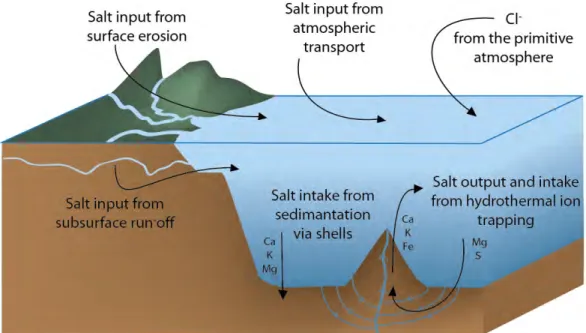
Salt in the ocean comes from the silicates’ erosion from surface and underground rivers run-offs. Rivers are 1000 times less concentrated in ions than the ocean as observed when comparing the ionic composition of fresh water (e.g., found on water bottles) and Table 1. Atmospheric circulation also transports salt ions from the land surface and volcanos. Salt ions concentration builds up once in the ocean as they do not react with marine minerals and they are left behind after evaporation. However, it has been shown from sediments analyses that ocean salinity has been (almost) stable for millions of year. The sources of ions (runoff) must be in equilibrium with sinks of ions (Figure I.2).
Figure I.2 The simplified geological cycle of salt
Two main sinks have been presented: life and hydrothermal ion trapping. Even if seaweeds, algae and fishes intake potassium (K) and magnesium (Mg) for their metabolism, only a small part is exported to the ocean floor where it can get trapped into the sediments. A greater proportion of calcium (Ca) is trapped inside shells and exported. Near the great ridges, water penetrates the oceanic crust and traps mainly Mg and sulphur (S), releasing Ca, K, iron (Fe) … The chloride ion (Cl
-) provenance is unclear as its concentration in the continental bedrock is very low, and therefore cannot be brought in the ocean by the rivers. It is though to come from the primitive atmosphere, and has stayed in the ocean since then. Sodium (Na+
) and Cl
have by far the greatest residence time in the ocean, 58 and 95 million years.
At present, the seawater salinity is on average 35 pss and the total quantity of salt represents 100 m3
per human being.
II. Importance of Salinity in Oceanography
As noted above, salinity definitions and measurement technics have evolved tremendously for over a hundred years as its scientific relevance has been increasingly recognised by scientists. As a matter of fact, (surface and subsurface) salinity is now recognized as one of the Essential Climate Variables (ECV) within the Global Climate Observing System (GCOS). It is a fantastic tool for tracking the freshwater cycle, water masses displacements and mixing. Salinity also impacts the ocean dynamics through density, as stated above. The following sections emphasise why scientists have expressed more and more interest in salinity.
II.1. A proxy to track water masses
Historically, scientists have used salinity as a water mass tracer. Water mass as defined by Tomczak (1999) is “a body of water with common formation history, having its origin in a physical region of the ocean”. Water masses are usually seen as objective physical entities that move around the ocean at different velocities. Subsurface water masses acquire their homogeneous characteristics at the sea surface or in the mixed-layer where they are formed. Characteristics are given by the atmosphere-ocean interactions (precipitations, evaporation, heating, cooling…). Salinity and temperature are “conservative properties” of theses masses unlike oxygen and nutrients which are consumed by biological processes. Once the water mass leaves the surface to reach deeper layers of the ocean, properties can only change by mixing with nearby water masses. Surface waters have properties varying much faster because of the atmospheric forcing fluctuations.
T-S plots (salinity as a function of temperature) are used to detect and define water masses, deduce their pathways and underline possible mixing with different water masses. For instance, the Tropical Pacific waters are marked by very high salinity whereas the Antarctic Intermediate Waters are characterised by low salinity and lower temperatures (see Figure II.1).
Figure II.1 T–S diagrams of 7 stations in the Pacific Ocean corresponding to thermocline waters of the Pacific Ocean: NE, NW, SE, SW Central Pacific waters (i.e. ECPNE, ECPNW, ECPSE ECPSW), N and S Equatorial Pacific waters (i.e. EEPN, EEPS), N and S Tropical Pacific waters (i.e. ETPN, ETPS), Antarctic Intermediate waters (EAAI) and N Pacific Intermediate waters (EIPN). From Fieux, 2010.
II.2. A marker for frontal regions
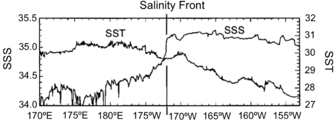
Salinity can also be a good proxy for frontal regions because its interactions with the atmosphere are not as strong as those of temperature. Broad scale surface salinity fronts are indeed usually sharper than temperature fronts, for instance the one observed along the equator by Rodier et al. (2000) in Figure II.2. This particular front will be further described in Section I.12. Strong and fast atmospheric responses to surface temperature fronts reduce their strength. Moreover, because the spatial scale of the atmospheric fronts are much larger than the oceanic ones, the gradient between the sea surface temperature and the air just above can be steep. Static stability is reduced on the warmer side of the front enhancing vertical mixing and winds. The opposite occurs on the cooler side of the front. Therefore, the atmosphere tends to weaken sharp temperature fronts whereas there is no direct atmospheric response to salinity fronts. Examples of salinity front analyses can be found in Picaut et al. (2001) for the western equatorial Pacific Ocean and in Reverdin et al. (1994) for the North Atlantic Ocean.
Figure II.2 Zonal distribution of high-resolution SST and SSS data collected from a TSG instrument during the September-October 1994 FLUPAC cruise along the equator (From Rodier et al., 2000). Note the sharp front in SSS and the lack of corresponding front in SST near 172°W.
II.3. A tool to estimate the freshwater cycle
Salinity is also thought to be a useful freshwater cycle proxy. Changes in the global hydrological cycle could affect billion of people especially if they imply an intensification of droughts and floods.
The global hydrological cycle corresponds to the freshwater storage and movement between the oceans, the continents, the atmosphere and the cryosphere. Around 80% of this cycle occurs over the oceans (83% of total evaporation and 78% of total precipitations) (e.g. Schanze et al., 2010). However, the ocean is vast and water fluxes are highly under-sampled. Sparse direct measurements are taken at moorings (such as TAO, RAMA, TRITON, PIRATA) and during oceanographic cruises (e.g. dedicated SPURS campaigns). Evaporation and Precipitations are very difficult to measure on the long term and global scale and are often derived from other variables with the help of models (i.e. reanalyses, models). In the early 2000’s, the development of satellite based microwave measurement of precipitations and latent heat flux improved our knowledge of large-scale fields. Yet uncertainties in the global hydrological cycle remain large. Using the optimal combination of independent estimates from satellites and in situ over the global ocean, fresh water transport can be assessed. Over the 1987-2006 period Schanze et al. (2010) found 13±1.3 Sv from evaporation, 12.2±0.2 Sv from precipitations and around 1.25±0.1 Sv. from river runoffs (Dai et al., 2009) exhibiting a net imbalance within error estimates. Looking at faint long-term changes in the hydrological cycle using atmospheric data is highly challenging due to large uncertainties (Lagerloef et al., 2010).
Figure II.3 Schematic of the global water cycle. Reservoir estimates represent storages in 103 km3, flux estimates represent transports in Sverdrup (106 m3 s-1) and values within boxes represent the approximate percentage of total storage for the global surface. Adapted from Schmitt (1995) and Schanze et al. (2010) by Paul Schanze.
Several studies have underlined the possible use of ocean surface salinity as an inverse rain gauge [e.g. Schmitt et al., 2008; Lagerloef et al., 2010]. To the first order, the freshwater cycle is reflected on the surface salinity fields. For instance a small 0.2 pss salinity decrease in a 35m depth mixed layer is equivalent to a notable 20% increase in precipitations (in common regions where the mean salinity and precipitaion are of the order of 35 pss and 1m/year, respectively). However, it remains challenging to link surface salinity with freshwater fluxes. Salinity is not solely driven by freshwater fluxes but also by complex upper ocean dynamical processes as will be presented in the following sections.
Delcroix et al (1996) found correspondent patterns of standard deviation of in-situ surface salinity and satellite derived precipitations in the heavy rainfall regions of the tropical Pacific. The Empirical Orthogonal Function (EOF) analysis of both parameters showed their link at the seasonal and interannual timescales. The authors also argued that surface salinity could be used to determine the phasing of precipitations changes but not the magnitude at both timescales.
Yu (2011) investigated the relation between the difference of Evaporation and Precipitations (E-P) and surface salinity on the seasonal timescales for the global ocean. From observations, Yu (2011) found E-P controlling salinity in only two regions: where P is strongly dominant (tropical convergence zones) and where E is strongly dominant (western North Pacific and Atlantic). Within these regions, E-P accounts for 40-70% of the surface salinity variance. More recently, Vinogradova and Ponte (2013) studied the interaction between salinity and the freshwater fluxes using a numerical model assimilating observations. They found on average a non-negligible part of salinity variability due to upper ocean processes, which correlates poorly to freshwater fluxes. At the global scale they showed a quasi non-existent relation between salinity and E-P. At the seasonal timescales, results are consistent with what was found earlier by Yu (2011)
At longer timescales, Durack and Wijffels (2010) looked at salinity variations and their link to E-P. They showed a strong connection between basin-wide averaged salinity and E-P in simulations from the Coupled Model Intercomparison Project (Phase 3; CMIP3). They put to light a 50-year trend pattern in salinity resembling what we can expect from an intensification of the global water cycle under global warming. The increasing difference in salinity between the Atlantic and Pacific Oceans is thought to be a remarkable indicator of the intensifying water cycle. (Salinity differences between the Atlantic and Pacific Oceans are discussed below.) Terray et al. (2012) focused on the tropical oceans over the late twentieth century with both observations and model simulations. They also concluded on a strengthened marine tropical hydrological cycle deduced from surface salinity variations, which they linked to anthropogenic forcing via detection / attribution methods.
II.4. The Seawater Equation of State
We have noted earlier that salinity measurements are primordial to compute another critical physical quantity: density. Seawater absolute density is (almost never) measured directly. Oceanographers use relative density anomaly (σ) computed from measurements of temperature (T), salinity (S) and pressure (P). The relative density is computed relative to standard seawater of known composition as shown below.
The Gibbs equation gives us the empirical relation between ρ and salinity (S), temperature (T) and pressure (P).
σ = ρ(ssample, T, P)
Because of its effect on density, salinity plays a key role in the ocean dynamics influencing dynamic height anomaly (and thus geostrophic currents), vertical mixing, subduction, etc. Subtle changes in salinity can lead to strong density anomalies as shown in
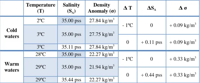
Table II.1. A temperature change of 1ºC corresponds to a change in salinity of 0.11 and 0.44 pss for cold (2-3°C) and warm (28-29°C) waters, respectively. This underlines the deeper effect of salinity changes on density in cold waters.
Temperature (T) Salinity (SA) Density Anomaly (σ) Δ T ΔSA Δ σ Cold waters 2ºC 35.00 pss 27.84 kg/m3 - 1ºC 0 + 0.09 kg/m3 3ºC 35.00 pss 27.75 kg/m3 0 + 0.11 pss + 0.09 kg/m3 3ºC 35.11 pss 27.84 kg/m3 Warm waters 28ºC 35.00 pss 22.27 kg/m3 - 1ºC 0 + 0.33 kg/m3 29ºC 35.00 pss 21.94 kg/m3 0 + 0.44 pss + 0.33 kg/m3 29ºC 35.44 pss 22.27 kg/m3
Table II.1 Changes in density for a 1-degree change in temperature in warm and cold waters, and equivalent salinity change for the same change in density.
Dynamic height anomaly relative to a given reference level is commonly deduced from temperature and salinity fields and can present great differences when using different methodologies. When salinity profiles were sparse, the traditional methodology was to use the available temperature profiles and mean climatological T-S curves (Emery and Wert, 1976). However, these climatological TS curves are not as stable as previously thought, especially near the surface, leading to dynamic height computation errors. These different approaches can result in large errors in dynamical height anomalies and thus in geostrophic currents and transports (e.g., Delcroix et al., 1987; Menkes et al., 1995; Ueki et al., 2002). For example in the equatorial Pacific (at 165°E), the effect of variability in the mean TS curves can result in errors of the order of 6 dyn.cm and 10 cm/s in surface dynamic height and geostrophic current, respectively. The Kessler/ linear TS-scheme approach led to a net improvement when computing dynamic height from surface salinity data, mean TS curves above the thermocline and the mean T-S relationship only below the thermocline (Kessler and Traft, 1987). Ideally,
both salinity and temperature profiles are needed simultaneously to get the dynamic height, which has been made possible in the recent decades (see Section III).
II.5. Role on deep waters formation (high latitudes)
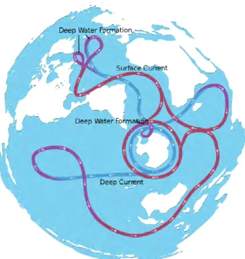
The Meridional Overturning Circulation (MOC) is the global circulation responsible for a large part of oceanic heat redistribution (Figure II.4). Warm waters are advected from low to high latitudes through western boundary currents. Cold waters are transported in the opposite direction in depth through the North Atlantic Deep Waters and Antarctic Bottom Waters. The MOC is mainly caused by temperature and salinity horizontal and vertical gradients but also winds. Salinity is of central importance in the deep convection processes by which deep waters are formed. The best illustration is the lack of deep convection in the North Pacific Ocean because of its low salinity. Moreover, studies have suggested that the North Atlantic MOC could be weakened due to an increase in fresh water in the northern North Atlantic, possibly linked to the observed ice melting acceleration from the arctic region (Rahmstorf, 1995; Manabe and Stouffer, 1995).
Deep convection occurs in the open ocean, along the coasts and over the continental shelves. Salinity plays an active role mostly in the open ocean deep convection; this has been observed in the Nordic, Labrador, Mediterranean, Weddell and Ross seas. Some evidence also shows probable open ocean deep convection in the Irminger Sea. However, the coastal deep convection in the Labrador Sea seems to be the most efficient process that produces MOC deep waters (Spall and Pickard, 2001).
Figure II.4 Schematic representation of the meridional overturning circulation by Van
de Sande (http://wanderingabout.com).
Open-ocean deep convection occurs seasonally in early winter when the wind curl is maximum. The movement of polar cyclonic gyres are strengthened and more isopycnals reach the surface. Surface waters become heavier under the action of atmospheric cooling and brine rejection from sea ice formation. Under these extreme conditions convective instabilities grow (Marshall and Schott, 1999). Deep convection takes place through a set of “plumes” of typically 1 km diameter and surrounding eddies. The heaviest waters are formed through this process.
Atmospheric conditions imprint their characteristics on the diving waters and again salinity can be used as a tracer as shown by Dickson et al. (2002).
II.6. Role on mixed layer via barrier layer formation (low latitudes)
Barrier layers exist in all oceans, mostly in the tropics, and the largest ones are found in the western Pacific Ocean (de Boyer Montégut et al., 2007). A large volume of waters above 28ºC can be found there from the surface to around 100m depth. This warm water body is called the “western Pacific warm pool”. Other warm pools exist such as the one off the coast of Panama. The warm pool is associated with low surface salinity waters west of 170ºE
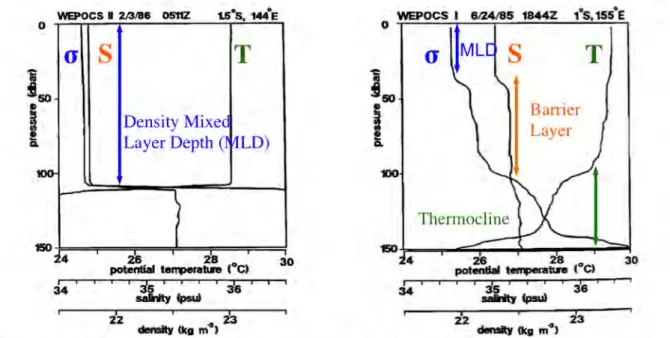
called “the fresh pool” (Figure IV.3; Delcroix and Picaut, 1998). In contrast with temperature, steep vertical salinity gradients are most often found in the first 50 meters of the fresh pool. The mixed layer is therefore controlled in this region by haline stratification. The layer between the base of the mixed layer (and halocline) and the thermocline is called “the barrier layer” (Lukas and Lindstrom, 1991; cf. Figure II.5).
Figure II.5 Potential temperature, salinity and potential density from CTD profiles at 1.5ºS, 144ºE in February 1986 (Left) and at 1ºS, 155ºE in June 1985 (Right). The left panel shows a mixed layer under “normal” conditions and the right panel shows the presence of a barrier layer. (Adapted from Lukas and Lindstrom, 1991)
A subtle balance between surface forcing, vertical mixing and large-scale dynamical processes is associated with the formation and maintenance of the barrier layer (Lukas and Lindstrom, 1991). They argued that the oceanic convergence described above brings higher salinity waters from the equatorial cold tongue. These waters subducting below the fresh pool create a strong halocline and the barrier layer. The convergence and subduction processes were also pointed out in numerical studies (Vialard 1998ab). However, Cronin and McPhaden (2002) referred to this mechanism as a maintaining process rather than a formation one. Temporal phasing was found between the barrier layer thickness and the precipitations anomalies underlying the importance of dynamical processes in the barrier layer variability (Ando and McPhaden, 1997). Cronin and McPhaden (2002) summarized four different mechanisms for the formation of barrier layer as: the local surface processes (heavy rain, low
wind, etc…), dynamic processes (subduction and advection) and the salinity front “tilting/shearing” under the effect of westerly wind bursts. These mechanisms were tested against observations by Bosc et al. (2009) during the 2000-2007 period.
The salinity barrier layer has an impact on atmosphere-ocean interactions. As salinity shoals the mixed layer, wind-forcing momentum and surface heating are distributed over a shallower layer and are thus more efficient (Vialard et al., 1998b). Furthermore, the barrier layer isolates the warm pool from cold waters below, reducing the impact of vertical mixing and entrainment. The warm pool is also isolated from the cold tongue waters by a zonal salinity front (Rodier et al., 2000; Picaut et al., 2001). Studies have also shown the importance of the barrier layer in the onset of the greatest mode of variability in the Pacific Ocean: the El Niño Southern Oscillation (ENSO). The barrier layer’s presence leads to an increase in temperature for instance by up to 0.8ºC during the 1997-1998 ENSO event (Lukas and Lindstorm, 1991, Vialard et al. 2002). Vialard et al. (2002) also found an increase by up to 0.2 m.s-1
in the surface current during the same ENSO experiment.
II.7. Salinity assimilation and impact on ENSO prediction
The effect of surface salinity assimilation in the model performance has been investigated by several studies. The assimilation of surface salinity alone has been found not to be sufficient to correct subsurface salinity biases (Reynolds et al., 1998). Using a complex assimilation method based on the Kalman filter theory and twin experiment approaches, Durand et al. (2002) showed the constraint of salinity related variables by assimilating surface salinity. In particular, the zonal velocity and the barrier layer were particularly better simulated during ENSO events. (The crucial influence of both etrms on ENSO will be described in following sections). Moreover, a reduction in precipitations estimation errors emerged when assimilating surface salinity data into an ocean model (Yaremchuk, 2006). With an assimilation scheme similar to the one used by Durand et al. (2002), experiments were carried out to evaluate the assimilation of simulated data from SMOS and Aquarius/SAC-D (Tranchant et al., 2008). The authors showed an improvement of their forecasting system and underlined the importance of specifying the observation error. At the time of writing, no published results can be found on assimilating satellite based salinity data. Assimilating surface salinity in a hybrid-coupled model leads to an increased correlation for 6-12 month forecasts by 0.2-0.5 and a reduction RMS error by 0.3ºC-0.6ºC (Hackert et al., 2011). The forecast of ENSO events is also improved.
Note that surface salinity can also be used as a statistical proxy to help predict ENSO (Ballabrera-Poy et al., 2002). Surface salinity does not impact ENSO now-casting (lag 0) but does increase the predictability of ENSO with lags from 6 to 9 months.
III. In situ S data Programs
Before the 1990s, salinity measurements in the open tropical oceans remained rather sparse in space and time. Most pre-1990 salinity measurements were made by Voluntary Observing Ships (VOS, Figure III.1 right) and sporadic oceanographic cruises. On VOS, bucket samples were usually collected by ship officers every 100 to 200 km and stored in bottles. Salinity was then measured in an oceanographic laboratory a few weeks later. A key VOS program was developed by ORSTOM (now called IRD) in Nouméa, New Caledonia, by the end of the 1960’s (see Donguy and Hénin, 1976). This program, still ongoing, is now part of the French SSS Observation Service described in Section 2.
Following the strong 1982-1983 ENSO event, the Tropical Ocean Global Atmosphere (TOGA) program (1985-1994) was created as a major component of the World Climate Research Program (WCRP). One of the objectives of the TOGA program was “to provide the scientific background for designing an observing and data transmission system for operational predication”. Observing systems have been strongly developed since. Automatic ThermoSalinoGraph (TSG) instruments were installed on the VOS (Figure III.1) in order to increase the spatial resolution of along track data (Hénin and Grelet, 1996). TSG were also installed on moorings (McPhaden et al., 1990) to produce long-term high temporal resolution salinity measurements. Ship tracks and moorings will be described in more details in the Data section.
Figure III.1 Left: Thermosalinograph installed on R.V. Nokwanda. Right: R.V. Rio Blanco (photos: C. Diverrès, IRD). Adapted from the French SSS observation Service web site.
TOGA decade induced improvements in monitoring mainly involve near-surface observations. Apart from the CTD cast data, salinity has only been measured at different depth since the years 2000s, from autonomous Argo floats (Roemmich et Owens, 2000; Figure III.2) and eXpendable Conductivity Temperature Depth (XCTD) transects (Sprintall and Roemmich, 1999). Nowadays, the spatial distribution of salinity measurements at the surface and at different depth enables the production of gridded datasets such those used in the following chapters.
Figure III.2 Left: XCTD . Right: Argo deployment by the CSIRO (Photo A. Navidad)
Because salinity measurements at depth were so scarce before the last decade, most of the earlier studies examined the sea surface salinity. Even if gridded products with different depth levels are improving, their length depends on the Argo floats’ deployments and they do not go back before 2002. In this context, numerical modelling has become more and more attractive to study ocean and atmosphere processes. Indeed, model performances have improved greatly in the last decades and they provide a full set of data in the 4 dimensions on regular grid points. Moreover, coupled models are independent of observation and can provide climate projections. However, we must keep in mind that even when using numerical models, salinity observations are still vital to assess model performances.
IV. Description of SSS patterns – Mean state
Even though findings on salinity have been constrained to the observations’ scattering and model ability to reproduce salinity, the overall distribution of salinity and its large scale variability is rather well know thanks to numerous scientific studies. These studies were made possible by the scientists’ and institutions’ willpower to gather observations in databases available to everyone such as Levitus (1982) and following atlases. Many studies will not be cited in this manuscript. This poorly expresses my gratitude to the salinity “early explorers” for all their baseline studies.
This section is a literature review of what is known about the salinity mean state salinity in the Global Ocean, continuing with a focus on the tropical Pacific Ocean.
IV.1. Mean SSS in the Global Ocean
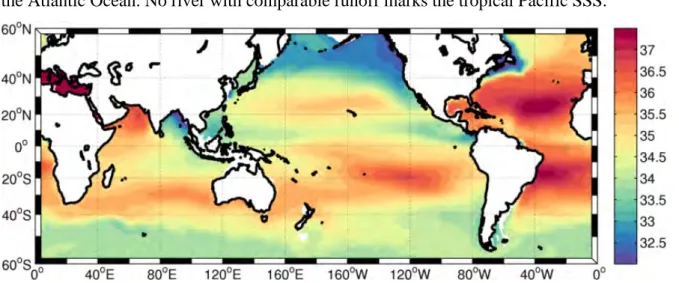
The mean surface distribution of salinity reveals patterns within basins but also from one basin to another (Figure IV.1). The Atlantic Ocean is significantly saltier than the Pacific Ocean even though they have similar large-scale fields. In both oceans, to the first order, the salinity distribution corresponds to the mean distribution of Evaporation minus Precipitations and River runoff (E-P-R). Low salinity regions roughly correspond to the Intertropical Convergence Zones (ITCZ) and South Pacific Convergence Zone (SPCZ) where precipitations are high and wind low. High Salinities are located in the subtropical basin centre, where evaporation is dominant. The river runoffs affect surface salinity as shown by the well-marked plumes of the Amazon, and to a lesser extent the Congo and Niger rivers in the Atlantic Ocean. No river with comparable runoff marks the tropical Pacific SSS.
Figure IV.1 Global map of surface salinity from the ISAS dataset (described in Chapter 2) averaged over 2004-2012.
As stated earlier, the Atlantic Ocean is on average a few pss saltier than the Pacific Ocean. Evaporation is directly linked to the relative humidity of the air above the sea surface. The Atlantic is under the influence of dry continental air and evaporation is intense (Schmitt et al., 2008). Moisture from the Atlantic Ocean is then transported across Central America to the Pacific Ocean in air masses advected by the Trade Winds (Weyl, 1968). Evaporation in the Pacific Ocean cannot therefore be as strong as in the Atlantic. As a consequence, evaporation dominates precipitations in the equatorial Atlantic basin whereas the equilibrium is reversed in the equatorial Pacific basin.
The Indian Ocean is very peculiar with a strong zonal gradient across the Indian subcontinent. Very salty waters are found in the Arabian Sea and very fresh waters in the Bay of Bengal. On the one hand, the salty waters can roughly be explained by the advection of very high salinity from the Red Sea through the Gulf of Aden and from the Persian Gulf. On the other hand, the Bay of Bengal’s extremely fresh waters result from both extreme rainfall and the Ganges and Brahmaputra rivers runoff.
Many studies have tried to understand the reasons for these mean salinity patterns. Near surface salinity is a balance of surface fresh water fluxes, advection in the three directions and other processes such as turbulence, diffusion etc.
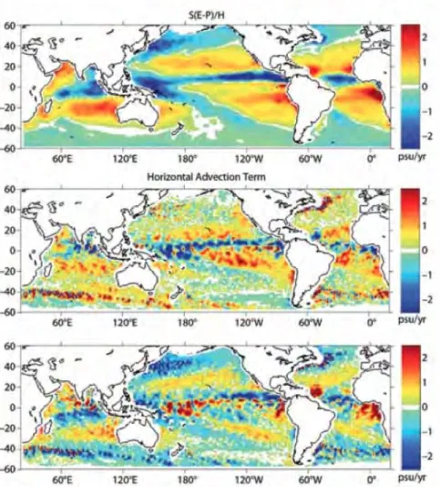
Based on satellite and other in situ estimates, Johnson et al (2002) investigated the equilibrium between freshwater fluxes from the atmosphere and advective processes of the ocean. The mean horizontal salinity advection they found is qualitatively comparable to the surface processes in both large-scale magnitude and spatial variance (correlation of 0.63). They found however substantial differences in the details. Excess of evaporation over the subtropical gyres more than compensates the excess of precipitations in the convergence zones (Johnson et al., 2002). There is also a poleward shift between the precipitations maxima and low salinity waters of the convergence zones, underlying the effect of horizontal advection (Delcroix et al., 1998). A similar shift is found between positive salinity advection and the compensating effect of the heavy precipitations (Johnson et al., 2002). Moreover, salinity advection over-compensates the salinity decrease in the tropical convergence zone (Lagerloef et al., 2010,Figure IV.2). Analogous processes are observed in the subtropical evaporation- dominated regions with shifts between the evaporation and salinity maxima (e.g. Delcroix and Henin, 1991). A shown on Figure IV.2, there is no balance in this region
between observed salinity divergence and surface fluxes suggesting the importance of inaccuracies and the other processes (Lagerloef et al., 2010).
Figure IV.2 Top: Atmospheric forcing term averaged over 2005-2008 using Global Precipitations Climatology Project (GPCP) and “Objectively Analysed” Ocean-Atmosphere flux (OAFlux) products (both will be described in Chapter 2). Middle: Horizontal salinity advection for the same years using Near real-time Global Ocean Surface Currents (OSCAR). Bottom: The difference field. From Lagerloef et al (2010).
Differences between surface forcing and horizontal advection (Figure IV.2) do not only represent the processes at work at the mixed layer base but also unknown bias errors in the surface forcing, horizontal advection and the salinity trend (depending greatly on the timeseries length). The errors to the salinity transport are difficult to specify especially because of the lack of SSS data. The eddy fluxes are not sampled in this study (using climatologic salinity) and are thought to be of prime importance in the salinity transport in the equatorial Pacific (Vialard et al., 2002).
IV.2. Mean SSS in the tropical Pacific Ocean
The tropical Pacific Ocean presents specific regional features in its surface salinity distribution such as the low salinity in the ITCZ, SPCZ and western Pacific warm pool as well as salinity maxima centred on 15ºN and 20ºS.
Along the equator, the surface salinity increases from the American coast to the central Pacific and decreases from there to the western boundary (Figure II.2, Figure IV.3 and Figure V.1). The unsteady decrease creates a steep surface salinity gradient and a front around 165°E. To the west of this front low salinity waters form the fresh pool mentioned earlier (Delcroix and Picaut, 1998).
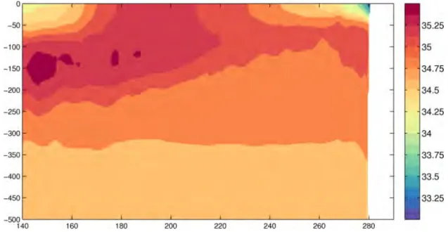
Figure IV.3 Longitude against depth salinity field along the equator averaged over 2004-2012, as obtained from the ISAS dataset (described in Chapter 2).
The low salinity waters of the fresh pool extend to 15ºS in the South Pacific Convergence Zone (Figure IV.1). A secondary surface salinity front is present between the southeast oriented fresh waters associated with heavy precipitations from the SPCZ and the westward oriented salty waters of the south Pacific salinity maximum advected by the southern branch of the South Equatorial Current (SEC) (Gouriou and Delcroix, 2002). The surface temperature field does not show any significant front with quasi-zonally oriented isotherms. Similarly, fresh waters are found roughly in the ITCZ region (5-10ºN, 120-140ºW) under the effect of strong precipitations and low salinity waters advected by the NECC from the west (Delcroix and Hénin, 1991).
The surface salinity absolute minimum (below 33.5 pss) spreads roughly from the American coast to 120ºW and between the equator and 10ºN (Figure IV.1; Figure IV.3). These low salinity waters are trapped between two distinctive systems: the eastern Pacific warm pool and the cold tongue of the equatorial Pacific upwelling system (Alory et al., 2012). This fresh pool corresponds mainly to an excess of precipitations over evaporation under the ITCZ and freshwater from the Andes and Caribbean regions.
Away from these SSS minima, large-scale high-salinity cores are centred within about 15-30° latitude in each hemisphere of the Pacific Ocean (Figure IV.1). Theses cores are also present in each hemisphere of the Atlantic Ocean and most studies have focused either on their global scale signature or on the North Atlantic core. These analyses have pointed out a 5 to 10º latitude shift between the cores and the evaporation-precipitations maxima due to the wind-driven Ekman salt transport (e.g., Delcroix and Hénin, 1991; Foltz and McPhaden, 2008; Qu et al., 2011).
V. SSS variability in the tropical Pacific Ocean– a brief
literature review
As presented above, salinity is affected by atmospheric forcing, advection and mixing. In consequence, salinity shows variability at all time and space scales. In this section, we give examples of salinity variability in the tropical Pacific Ocean from small time/space scales to changes over multiple decades.
V.1. Small time/space scales
Several studies have tried to quantify SSS variability at scales under a month and a few km. However, few measurements can be of use for this matter. Indeed, times series with very high resolution are needed such as for instance VOS-TSG (for the space-scale) and TAO-TSG (for the temporal-scale). Lagerloef and Delcroix (2001) examined high-resolution data sets and also focused on sampling errors from different resolutions in the western Pacific warm-pool region only. They under-sampled SSS from the original VOS along-tack 0.02º resolution to 2º samples and from the original TAO from under an hour resolution to 10-day sample. The sampling error was found to be less than 0.1 pss in most cases but reaches 0.3 in the vicinity of steep SSS fronts. Delcroix et al. (2005) expanded this study to the three
tropical oceans along 13 well-sampled ship tracks. Standard deviations of the VOS SSS over 0.5º, 1º and 2º degrees of latitude and 1º, 2º and 5º degrees of longitude intervals were computed in order to estimate the SSS variability at these ‘small’ spatial scales (Figure V.1).
Figure V.1 Examples of high-resolution SSS observations recorded along the equator during 9-18 October 1994, and standard deviations of SSS computed over 0.5º, 1º and 2º longitudes. From Delcroix et al. (2005).
Studies mentioned above all showed small-scale variability of the order of 0.1 pss but as observed by Lagerloef and Delcroix (2001), occasionally reaching 0.2 to 0.4 pss. Furthermore, the 10-and 30-day standard deviations from the TAO SSS are usually less than 0.2 but reached 0.5 during the 1994 ENSO event. These errors are associated with sharp SSS front but also heavy precipitations in the western half of the equatorial Pacific Ocean. Results from Lagerloef and Delcroix (2001) and Delcroix et al. (2005) underline the high salinity variability at small scales, which could affect the interpretation of irregularly collected observations and therefore studies at all scales.
V.2. Intraseasonal time scales
Intraseasonal variability is considered as corresponding to a temporal scale of variability of about a month and to spatial scale of a thousand kilometres. TIWs (Tropical
Instability Wave) were first characterized by meanders in the meridional SST front as seen from satellites with 1000km wavelength and with a 25-day period in the eastern equatorial Pacific (Legeckis, 1977). The TIW are westward propagating waves and exist in the equatorial regions of both the Atlantic and Pacific Oceans. Following Kessler et al. ’s (1996) study, Lyman et al (2007) described the TIW of the Pacific Ocean with observations from the TAO buoy array. They identified two distinct TIWs with periods of 17- and 33-day, with similar characteristics to a Yanai/surface trapped instability and an instable first meridional mode Rossby wave. Reinforced by evidence from modelling, the 17-day TIW was found to imprint its variability within two degrees off the equator on meridional velocity and subsurface temperature. In constrast, the 33-day TIW variability is reflected on subsurface temperature at 5º North of the Equator.
Figure V.2 7-day averages of SSS (pss) derived from Aquarius/SAC-D (colour shading in a-c), SST (ºC, contours in a), surface current (m/s, vectors in b) and sea surface height anomaly (cm, SSHA) (contours in c) centred on December 18, 2011. Surface currents are 10-day average centered on Dec. 18. From Lee et al. (2012).
The first Aquarius/SAC-D measurements reveal SSS variability linked to the TIWs (Lee et al., 2012). (Note that SMOS quasi-repeat period is 18-day, and unfortunately cannot
be of much help to study with accuracy the TIW). The SSS structures captured by Aquarius (Figure V.2) match the TIW ones obtained from SST and sea surface height (SSH). The three parameters have meridional gradients and therefore are affected by the TIWs differently. The maximum meridional gradients of SSS, SSH and SST are centred on the equator, 2ºN and 4ºN respectively. High resolution SSS is therefore ideal to detect and study the 17-day TIW. TIWs show some variability in their intensity which could impact locally SSS. Indeed, the TIWs activity depends on the equatorial current shear. The likely role of TIW on the salt budget is still an open question.
V.3. Seasonal variability
The seasonal variability of salinity has been shown to account for about 53% of the total suface salinity variability in the tropics (Johnson et al., 2002). The maximum seasonal SSS variability in the tropical Pacific is located in the ITCZ, SPCZ and western Pacific (Delcroix and Hénin, 1991; Delcroix, 1998) where the seasonal cycle characterises more than half of the signal (Delcroix et al., 2005). In some parts of the Pacific Ocean, the seasonal cycle represents only less than 25% of variance, highlighting variability dominated by other scales.
Observed sea surface salinity variability at the seasonal time scale reveals a 6-month lag between cycles along the ITCZ and SPCZ. Salinity is minimum in October in the ITCZ and in April in the SPCZ (Delcroix, 1998). Seasonal salinity variations in the ITCZ are consistent with 2- to 3-month lags with the variations of precipitations (Delcroix and Henin, 1991; Delcroix et al., 2005). Gouriou and Delcroix (2002) focused on the SCPZ and found SSS variations lagging precipitations by around 3 months with maximum intensity over the exact same area. Indeed, the well-known ITCZ and SPCZ atmospheric seasonal cycles show high deep convection activity during boreal and austral winter respectively and low deep convection activity during summer (Meehl, 1987; Vincent, 1994).
Figure V.3 (left) spatial patterns and (right) associated time function of the 1st
mode of the Empirical Orthogonal Function (EOF) of the seasonal surface (top) temperature and (bottom) salinity. Computed over 1962-1993 and 1973-1992 respectively. The time functions correspond to the average month by month (solid line) bracketed by ±1 monthly standard deviation (dashed lines). The units are defined by the EOF so the product of the spatial pattern and time series gives ºC for the temperature and pss for the salinity. From Delcroix (1998)
Despite the unmistakeable impact of surface fluxes on seasonal variability, Delcroix (1998) evidenced the probable effect of salt advection seasonal variability from both the North and South Equatorial Counter Currents (NECC and SECC), which have well marked seasonal cycles themselves. In the ITCZ, salinity seasonal variations are coherent with a 2- to 3-month lag with maximum freshwater eastward flow of the NECC (Delcroix and Henin, 1991; Delcroix et al., 2005). Furthermore in the central part of the Basin, the meridional Ekman advection is in phase with the precipitations seasonal variability (Delcroix and Henin, 1991). The freshwaters from the equatorial upwelling advected by the Ekman currents could therefore reinforce the precipitations’ impact.
Note that the 2- to 3- month lag between maximum E-P and minimum SSS (with E-P leading) can be explained mostly by the effect of E-P on salinity changes (dS/dt) and not by salinity directly, as discussed by Hires and Montgomery (1972; see also Equation II.1 below).
V.4. Interannual variability
ENSO is the principal variability mode of the Pacific Ocean at the interannual time scale. ENSO is an atmosphere-ocean coupled phenomena with a periodicity between 2 to 8 years. It includes a warm phase, El Niño, and a cold phase, La Niña (see Philander, 1985; 1990). The strength of El Niño / La Niña is usually estimated using the Southern Oscillation Indice (SOI), which corresponds to the normalized sea level pressure difference between Tahiti (French Polynesia) and Darwin (Australia) shown in Figure V.4.
Figure V.4 Time series of the SOI . Variability below 8-month has been filtered out. Data is derived using normalization factors derived from monthly values. Blue correspond to La Niña events and red to El Niño events. Downloaded from the National Center for Atmospheric Research (NCAR) Earth System Laboratory.
ENSO has been thoroughly studied using observed SST, SSH and other parameters. We will remind here conditions associated with the so-called normal, El Niño and La Niña situations (Figure V.5).
Figure V.5 Schematic plots of: (a) Normal, (b) El Niño and (c) La Niña conditions. Coloured surface contours represent the surface temperature. Back (white) arrows denote the
main equatorial atmospheric winds (oceanic currents). Adapted from
(http://pmel.noaa.gov/tao/elNiño/Niño-home.html)
When the tropical Pacific Ocean is under ‘normal’ conditions the warm pool is trapped to the west under the effect of the trade winds. Additionally, the warm pool provides heat for the deep atmospheric convection of the Walker ascending branch. In the east, the equatorial eastern Pacific upwelling system brings cold waters up and shoals the thermocline.
The relaxation of trade winds and/or westerly wind anomalies in the warm pool forces the fresh pool eastern edge convergence to move eastward. As a consequence, the warm and fresh waters from the warm pool spread in the central and in some cases in the eastern equatorial Pacific. Changes in temperature deepen the eastern thermocline and lessen its tilt leading to a weakening or complete shut off of the equatorial upwelling. Furthermore, the deep convection systems follow the warm waters modifying the Waker circulation. Wind stress convergence regions are also modified and the ITCZ and SPCZ both shift equatorward.
The La Niña conditions are analogous to the normal phase but intensified. The warm pool is shifted to its westernmost position and the SEC is intensified. Associated deep convection follows the warm pool back west and the Walker circulation is restored. The ITCZ and SPCZ both swing back poleward to their original positions.
The surface salinity ENSO signal was isolated using EOFs applied to a low-pass filtered SSS gridded field derived from in-situ measurements (Delcroix, 1998, see Figure V.6). The first EOF time function is highly correlated to the SOI with a 4-month lag. The associated spatial field shows a boomerang-shape of high-values (negative in their study). Changes in the warm pool reach 1 pss. More recent studies with longer time series including more numerous ENSO events obtain consistent patterns (e.g. Gouriou and Delcroix, 2002; Singh et al., 2011).
Figure V.6 Analogous to Figure V.3 but for the interannual signal. The dashed lines in the right panels correspond to the SOI.
Different analyses have focused on the processes behind the observed SSS interannual variability. The warm pool eastern edge convergence follows the ENSO cycle (Picaut et al., 2001). The oceanic convergence zone (i.e. zonal salinity front) is displaced east as the warm pool extends eastward during El Niño by zonal advection (Picaut et al., 1996; Cronin et al., 1998). The convective cells follow this displacement and sustain the salinity front (Picaut et al., 2001). The eastward warm pool displacement also increases the fetch of westerly winds over warm waters enhancing their penetration in the central equatorial Pacific Ocean. Furthermore, the weakening of the SEC during El Niño together with the anomalous eastward mass fluxes reduces the quantity of saline water subducting under the warm pool. This reduction erodes the barrier layer (Lukas and Lindstrom, 1991).
Moreover the zonal salinity gradient maximum (salinity front) associated with the barrier layer depth described earlier follows the warm pool displacements at the ENSO time scale (Delcroix and McPhaden, 2002; Bosc et al, 2009). Thick barrier layers in central and eastern Pacific precede El Niño MLT and precipitations anomalies by one or two seasons (Maes, 2006; Ando and McPhaden, 1997). The authors hypothesized that the barrier layer may contribute to an increase of the mixed layer temperature in the cold tongue region, which in turn increases precipitations.
During La Niña, waters in the central and eastern Pacific are unusually cold with dry conditions. The warm pool is confined to the westernmost part of the equatorial Pacific, the barrier layer develops only west of 160ºW (Ando and McPhaden, 1997).
Unlike SST, there is also a peak in interannual SSS variability located along the SPCZ main axis (Delcroix and Hénin, 1991; Gouriou and Delcroix, 2002). In the SPCZ region, SSS increases during an El Niño event whereas it decreases during a La Niña event with a magnitude twice as high as the seasonal cycle (Gouriou and Delcroix, 2002). Highest correlation was found between the secondary SSS front and the SOI with a 5-month lag. This variability is however not always as correlated with SOI. Indeed, authors pointed out the 1993-1995 unusual quasi-permanent El Niño conditions at the equator which had no impact on the secondary SPCZ front.
Under the SPCZ, Delcroix and Henin (1989) observed a strengthening of the SEC during the 1982-1983 El Niño. This underlines the importance of horizontal advection in the interannual displacement of the secondary SSS front. Gouriou and Delcroix (2002) found a northeast-southwest displacement of the SPCZ SSS front consistent with the atmospheric deep convection movements.
V.5. Decadal variability
The Pacific Decadal Oscillation (PDO, Hare, 1996) is believed to be the main decadal signal over the Pacific Ocean. The PDO is an oscillatory pattern of climate variability over the North Pacific (Mantua et al., 1997) with cold and warm phases north. The PDO index is based on an EOF analysis of the Pacific SST north of 20ºN (Figure V.8, bottom) but impacts the whole basin variability. The PDO embodies anomalous patterns in surface and subsurface temperature, sea level pressure and surface wind stress fields (Figure V.7), all rotating clockwise around the North Pacific Gyre (Zhang and Levitus, 1997). The warm phase shown on Figure V.7 (right panel) corresponds to cooler than average SST anomalies in the North-western Pacific and warmer than average on the American coast but also negative sea level pressure in the central part of the basin. The cold phase is roughly the opposite (Figure V.7, left panel).