O
pen
A
rchive
T
OULOUSE
A
rchive
O
uverte (
OATAO
)
OATAO is an open access repository that collects the work of Toulouse researchers and
makes it freely available over the web where possible.
This is an author-deposited version published in : http://oatao.univ-toulouse.fr/
Eprints ID : 12872
To link to this article : DOI :10.1007/978-3-319-04939-7_7
URL : http://dx.doi.org/10.1007/978-3-319-04939-7_7
To cite this version : Ciucci, Davide and Dubois, Didier and Prade,
Henri The Structure of Oppositions in Rough Set Theory and Formal
Concept Analysis - Toward a New Bridge between the Two Settings.
(2014) In: International Symposium on Foundations of Information and
Knowledge Systems - FolKS 2014, 3 March 2014 - 7 March 2014
(Bordeaux, France).
Any correspondance concerning this service should be sent to the repository
administrator: [email protected]
The structure of oppositions in rough set theory
and formal concept analysis
-Toward a new bridge between the two settings
Davide Ciucci1, Didier Dubois2, and Henri Prade2
1
DISCo, Universit`a di Milano–Bicocca, viale Sarca 336 U14, 20126 Milano (Italy), [email protected]
2
IRIT, Universit´e Paul Sabatier, 118 route de Narbonne, 31062 Toulouse cedex 9 (France), {dubois, prade}@irit.fr
Abstract. Rough set theory (RST) and formal concept analysis (FCA) are two formal settings in information management, which have found applications in learning and in data mining. Both rely on a binary re-lation. FCA starts with a formal context, which is a relation linking a set of objects with their properties. Besides, a rough set is a pair of lower and upper approximations of a set of objects induced by an in-distinguishability relation; in the simplest case, this relation expresses that two objects are indistinguishable because their known properties are exactly the same. It has been recently noticed, with different con-cerns, that any binary relation on a Cartesian product of two possibly equal sets induces a cube of oppositions, which extends the classical Aris-totelian square of oppositions structure, and has remarkable properties. Indeed, a relation applied to a given subset gives birth to four subsets, and to their complements, that can be organized into a cube. These four subsets are nothing but the usual image of the subset by the relation, together with similar expressions where the subset and / or the relation are replaced by their complements. The eight subsets corresponding to the vertices of the cube can receive remarkable interpretations, both in the RST and the FCA settings. One facet of the cube corresponds to the core of RST, while basic FCA operators are found on another facet. The proposed approach both provides an extended view of RST and FCA, and suggests a unified view of both of them.
Keywords: rough set; formal concept analysis; square of oppositions; possibility theory.
1
Introduction
Rough set theory (RST) [31–33, 36, 35, 34] and formal concept analysis (FCA) [2, 41, 18, 17] are two theoretical frameworks in information management which have been developed almost independently for thirty years, and which are of particular interest in learning and in data mining. Quite remarkably, both rely on a binary relation. In FCA, the basic building block is a relation that links a set of objects with a set of properties, called a formal context. A rough set
is a pair of lower and upper approximations of a set of objects induced by an indistinguishability relation, objects being indistinguishable in particular when they have exactly the same known properties.
Besides, in a recent paper dealing with abstract argumentation [1], it has been noticed that in fact any binary relation is associated with a remarkable and rich structure, called cube of oppositions, which is closely related to the Aristotelian square of oppositions. The purpose of this paper is to take advantage of this cube for revisiting both RST and FCA in a unified manner. The expected benefit is twofold. On the one hand, it may provide an enriched view of each framework individually, on the other hand it should contribute to a better understanding of the relations and complementarities between the two frameworks.
The paper is organized as follows. In the next section, we present a detailed account of the structure of oppositions associated with a binary relation,which
is represented by a cube laying bare four different squares of oppositions, each
of which may be completed into hexagons in a meaningful way.This systematic
study substantially extends preliminary remarks made in [10, 1]. Then, Sections
3 and 4 respectively restate RST and FCA in the setting of this cube and its hexagons, providing an extended view of their classical frameworks.This leads to new results on the rough set cube and hexagons, which are then related
to previous results on oppositions in rough sets [6]. Similarly this leads to a
renewed presentation of results in FCA. Section 5, after surveying the various
attempts in the literature at bridging or mixing RST and FCA in one way or another, suggests new directions of research which can benefit from the unified view presented in this paper, before concluding.
2
Structure of oppositions induced by a binary relation
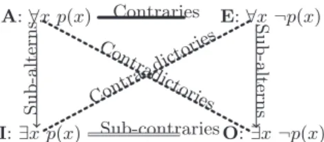
Let us start with a refresher on the Aristotelian square of opposition [30]. The traditional square involves four logically related statements exhibiting universal or existential quantifications: it has been noticed that a statement (A) of the form “every x is p” is negated by the statement (O) “some x is not p”, while a statement like (E) “no x is p” is clearly in even stronger opposition to the first statement (A). These three statements, together with the negation of the last one, namely (I) “some x is p”, give birth to the Aristotelian square of opposition in terms of quantifiers A : ∀x p(x), E : ∀x ¬p(x), I : ∃x p(x), O: ∃x ¬p(x), pictured in Figure 1. Such a square is usually denoted by the letters A, I (affirmative half) and E, O (negative half). The names of the vertices come from a traditional Latin reading: AffIrmo, nEgO). As can be seen, different relations hold between the vertices. Namely,
- (a) A and O are the negation of each other, as well as E and I; - (b) A entails I, and E entails O (we assume that there are some x); - (c) A and E cannot be true together, but may be false together; - (d) I and O cannot be false together, but may be true together.
Contraries A: ∀x p(x) E: ∀x ¬p(x)Sub-alterns Sub-contraries I: ∃x p(x) O: ∃x ¬p(x) Sub-alterns Contradict ories Contra dictories
Fig. 1.Square of opposition
Another well-known instance of this square is in terms of the necessary (✷) and possible (✸) modalities, with the following reading A : ✷p, E : ✷¬p, I : ✸p, O: ✸¬p, where ✸p =def ¬✷¬p (with p 6= ⊥, ⊤).
2.1 The square of relations
Let us now consider a binary relation R on a Cartesian product X × Y (one may have Y = X). We assume R 6= ∅. Let xR denote the set {y ∈ Y |(x, y) ∈ R}, and we write xRy when (x, y) ∈ R holds, and ¬(xRy) when (x, y) 6∈ R. Let Rt
denote the transpose relation, defined by xRty if and only if yRx, and yRtwill
be also denoted as Ry = {x ∈ X|(x, y) ∈ R}.
Moreover, we assume that ∀x, xR 6= ∅, which means that the relation R is serial, namely ∀x, ∃y such that xRy; this is also referred to in the following as the X-normalization condition. In the same way Rtis also supposed to be serial,
i.e., ∀y, Ry 6= ∅. We further assume that the complementary relation R (xRy iff ¬(xRy)), and its transpose are also serial, i.e. ∀x, xR 6= Y and ∀y, Ry 6= X.
Let S be a subset of Y . The relation R and the subset S, also considering its complement S, give birth to the two following subsets of X, namely the (left) images of S and S by R
R(S) = {x ∈ X|∃s ∈ S, xRs} = {x ∈ X| S ∩ xR 6= ∅} (1) R(S) = {x ∈ X|∃s ∈ S, xRs}
and their complements
R(S) = {x ∈ X|∀s ∈ S, ¬(xRs)}
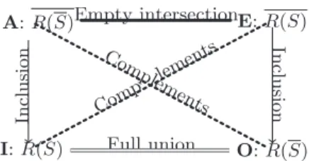
R(S) = {x ∈ X|∀s ∈ S, ¬(xRs)} = {x ∈ X| xR ⊆ S} (2) The four subsets thus defined can be nicely organized into a square of op-position. See Figure 2. Indeed, it can be checked that the set counterparts of the relations existing between the logical statements of the traditional square of oppositions still hold here. Namely,
- (a) R(S) and R(S) are complements of each other, as R(S) and R(S); they correspond to the diagonals of the square;
Empty intersection A: R(S) E: R(S) Inclusion Full union I: R(S) O: R(S) Inclusion Com plements Comp lements
Fig. 2.Square of oppositions induced by a relation R and a subset S
thanks to the X-normalization condition ∀x, xR 6= ∅. These inclusions are re-presented by vertical arrows in Figure 2;
- (c) R(S) ∩ R(S) = ∅ (this empty intersection corresponds to a thick line in Figure 2), and one may have R(S) ∪ R(S) 6= Y ;
- (d) R(S) ∪ R(S) = X (this full union corresponds to a double thin line in Figure 2), and one may have R(S) ∩ R(S) 6= ∅.
Conditions (c)-(d) hold also thanks to the X-normalization of R.
Note that one may still have a modal logic reading of this square where R is viewed as an accessibility relation, and S as the set of models of a proposition. 2.2 The cube of relations
Let us also consider the complementary relation R, namely xRy if and only if ¬(xRy). We further assume that R 6= ∅ (i.e., R 6= X × Y ). Moreover we have also assumed the X-normalization of R, i.e. ∀x, ∃y ¬(xRy). In the same way as previously, we get four other subsets of X from R. Namely,
R(S) = {x ∈ X|∃s ∈ S, ¬(xRs)} = {x ∈ X|S ∪ xR 6= X} (3) R(S) = {x ∈ X|∃s ∈ S, ¬(xRs)}
and their complements
R(S) = {x ∈ X|∀s 6∈ S, xRs}
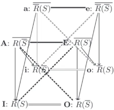
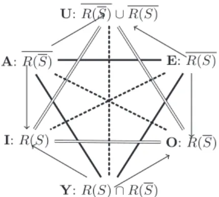
R(S) = {x ∈ X|∀s ∈ S, xRs} = {x ∈ X|S ⊆ xR} (4) The eight subsets involving R and its complement can be organized into a cube of oppositions [7] (see Figure 3). Similar cubes have been recently exhibited as extending the traditional square of oppositions in terms of quantifiers [10], or in the particular setting of abstract argumentation (for the complement of the attack relation) [1]. As can be seen, the front facet of the cube in Figure 3 is nothing but the square in Figure 2, and the back facet is a similar square associ-ated with R. Neither the top and bottom facets, nor the side facets are squares of opposition in the above sense. Indeed, condition (a) is violated: Diagonals do not link complements in these squares. More precisely, in the top and bottom
squares, diagonals change R into R and vice versa; there is no counterpart of condition (b), and either condition (c) holds for the pairs of subsets associated with vertices A-E and with vertices a-e, while condition (d) fails (top square), or conversely in the bottom square, condition (d) holds for the pairs of subsets associated with vertices I-O and with vertices i-o while condition (c) fails. For side facets, condition (b) clearly holds, while both conditions (c)-(d) fail. In side facets, vertices linked by diagonals are exchanged by changing R into R (and vice versa) and by applying the overall complementation. These diagonals express set inclusions: R(S) = {x ∈ X|∀s ∈ S, ¬(xRs)} ⊆ {x ∈ X|∃s ∈ S, ¬(xRs)} = R(S). In the same way, we have R(S) ⊆ R(S), R(S) ⊆ R(S), and R(S) ⊆ R(S), as pictured in Figure 3. i: R(S) I: R(S) O: R(S) o: R(S) a: R(S) A: R(S) E: R(S) e: R(S)
Fig. 3.Cube of oppositions induced by a relation R and a subset S
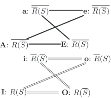
Moreover, the top and bottom facets exhibit other empty intersection re-lationships and full union rere-lationships respectively. Indeed in the top facet, e.g. R(S) ∩ R(S) = ∅, since R(S) = {x ∈ X | S ⊆ xR} and R(S) = {x ∈ X | S ∩ xR = ∅}. Similarly in the bottom facet, e.g. R(S) ∪ R(S) = X, since R(S) = {x ∈ X|∃s ∈ S, ¬(xRs)} and R(S) = {x ∈ X|∃s ∈ S, xRs}. This is pictured in Figure 4 (in order not to overload Figure 3).
Thus, while diagonals in front and back facets express complementations, they express inclusions in side facets, empty intersections in top facet, and full union in bottom facets.
It is important to keep in mind that the 4 subsets R(S), R(S), R(S), and R(S) (or their complements R(S), R(S), R(S), and R(S)) constitute distinct pieces of information in the sense that one cannot be deduced from the others. Indeed the conditions xR ⊆ S, S ∩ xR = ∅, S ⊆ xR, and S ∪ xR = X express the four possible inclusion relations of xR wrt S or S and define distinct subsets of X.
The 8 subsets corresponding to the vertices of the cube of oppositions can receive remarkable interpretations, both in the RST and FCA settings. As we shall see in Sections 3 and 4, the front facet of the cube corresponds to the core of RST, while basic FCA operators are on the left-hand side face. However, before
i: R(S) I: R(S) O: R(S) o: R(S) a: R(S) A: R(S) E: R(S) e: R(S)
Fig. 4.Top and bottom facets of the cube of oppositions
moving to RST and FCA, it is interesting to complete the different squares corresponding to the facets of the cube into hexagons, as we are going to see.
2.3 From squares to hexagons
As proposed and advocated by Blanch´e [4, 5], it is always possible to complete a classical square of opposition into a hexagon by adding the vertices Y =defI∧O,
and U =def A∨ E. It fully exhibits the logical relations inside a structure of
oppositions generated by the three mutually exclusive situations A, E, and Y, where two vertices linked by a diagonal are contradictories, A and E entail U, while Y entails both I and O. Moreover I = A ∨ Y and O = E ∨ Y. Conversely, three mutually exclusive situations playing the roles of A, E, and Y always give birth to a hexagon [10], which is made of three squares of opposition: AEOI, AYOU, and EYIU, as in Figure 5. The interest of this hexagonal construct has been rediscovered and advocated again by B´eziau [3] in the recent years in particular for solving delicate questions in paraconsistent logic modeling.
Applying this idea to the front facet of the cube of oppositions induced by a relation and a subset, we obtain the hexagon of Figure 5, associated with the tri-partition {R(S), R(S), R(S) ∩ R(S)}. Note that indeed R(S) = R(S) ∪ (R(S) ∩ R(S)) (since R(S) ⊇ R(S)). Similarly, R(S) = R(S) ∪ (R(S) ∩ R(S)). In Figure 5, arrows (→) indicate set inclusions (⊆). A similar hexagon is associated with the back facet, changing R into R.
Another type of hexagon can be associated with side facets. The one corre-sponding to the left-hand side facet is pictured in Figure 6. Now, not only the arrows of the sides of the hexagon correspond to set inclusions, but also the diag-onals (oriented downwards). Indeed R(S) ⊆ R(S) and R(S) ⊆ R(S). Moreover, since R(S) ⊆ R(S) and using the inclusions corresponding to the vertical edges of the cube, we get
R(S) ∪ R(S) ⊆ R(S) ∩ R(S),
A: R(S) U: R(S) ∪ R(S) E: R(S) O: R(S) Y: R(S) ∩ R(S) I: R(S)
Fig. 5.Hexagon associated with the front facet of the cube
R(S) ∪ R(S) ⊆ R(S) ∩ R(S). A: R(S) R(S) ∪ R(S) a: R(S) i: R(S) R(S) ∩ R(S) I: R(S)
Fig. 6.Hexagon induced by the left-hand side square
One may wonder if one can build useful hexagons from the bottom and top squares of the cube. It is less clear. Indeed, if we consider the four subsets involved in the bottom square, namely R(S), R(S), R(S) and R(S) (the top square has their complements as vertices), they are weakly related through R(S) ∪ R(S) = X, R(S)∪R(S) = X, R(S)∪R(S) = X and R(S)∪R(S) = X. Still R(S)∪R(S) or R(S)∪R(S) (or their complements in the top square, R(S)∩R(S) or R(S)∩R(S)) are compound subsets that may make sense for some particular understanding of relation R. Note that similar combinations changing ∩ into ∪ and vice versa already appear in the hexagons associated with the side facets of the cube, while
R(S) ∩ R(S) and R(S) ∩ R(S) are the Y-vertices of the hexagons associated with the front and back facets of the cube of oppositions. Besides, it would be also possible to complete the top facet into yet another type of hexagon by taking the complements of R(S) ∪ R(S) or of R(S) ∪ R(S), which clearly have empty intersections with the subsets attached to vertices A and a and to vertices E and e respectively. However, the intersection of the two resulting subsets, namely R(S) ∩ R(S) and R(S) ∩ R(S) is not necessarily empty. A dual construct could be proposed for the bottom facet.
In the cube of oppositions, three negations are at work, the usual outside one, and two inside ones respectively applying to the relation and to the subset - this gives birth to the eight vertices of the cube - while in the front and back squares (but also in the top and bottom squares) only two negations are at work. Besides, it is obvious that a similar cube can be built for the transpose relation Rt and a subset T ⊆ X, then inducing eight other remarkable subsets, now, in
Y. This leads us to assume the X-normalizations of Rtand Rt (= Rt), which is
nothing but the Y-normalizations of R and R (∀y, ∃t, tRy, and ∀y, ∃t′,¬(t′Ry)),
as already announced. We now apply this setting to rough sets.
3
The Cube in the Rough Set Terminology
Firstly defined by Pawlak [32], rough set theory is a set of tools to represent and manage information where the available knowledge cannot accurately describe reality. From an application standpoint it is used mainly in data mining, machine learning and pattern recognition [34].
At the basis of the theory, there is the impossibility to accurately give the intension of a concept knowing its extension. That is, given a set of objects S we cannot characterize it precisely with the available features (attributes) but, on the other hand, we can accurately define a pair of sets, the lower and upper approximations L(S), U (S), which bound our set: L(S) ⊆ S ⊆ U (S). The interpretation attached to the approximations is that the objects in the lower bound surely belong to S and the objects in the boundary region U (S) \ L(S) possibly belong to S. As a consequence we have that the objects in the so-called exterior region U (S) do not belong to S for sure.
The starting point of the theory are information tables (or information sys-tems) [31, 36], which have been defined to represent knowledge about objects in terms of observables (attributes).
Definition 1. An information table is a structure K(X) = hX, A, val, F i where: the universe X is a non empty set of objects; A is a non empty set of condi-tion attributes; val is the set of all possible values that can be observed for all attributes; F (called the information map) is a mapping F : X × A → val which associates to any pair object–attribute, the value F (x, a) ∈ val assumed by a for the object x.
Given an information table, the indiscernibility relation with respect to a set of attributes B ⊆ A is defined as
xIBy iff ∀a ∈ B, F (x, a) = F (y, a)
This relation is an equivalence one, which partitions X in equivalence classes xRB. Due to a lack of knowledge we are not able to distinguish objects inside
the granules, thus, it can happen that not all subsets of X can be precisely characterized in terms of the available attributes B. However, any set S ⊆ X can be approximated by a lower and an upper approximation, respectively defined as:
LB(S) = {x : xRB⊆ S} (5a)
UB(S) = {x : xRB∩ S 6= ∅} (5b)
The pair (LB(S), UB(S)) is called a rough set. Clearly, omitting subscript B, we
have, L(S) ⊆ S ⊆ U (S), which justifies the names lower/upper approximations. Moreover, the boundary is defined as the objects belonging to the upper but not to the lower: Bnd(S) = U (S) \ L(S) and the exterior is the collection of objects not belonging to the upper: E(S) = U (S). The interpretation attached to these regions is that the objects in the lower approximation surely belong to S, the objects in the exterior surely do not belong to S and the objects in the boundary possibly belong to S.
Several generalizations of this standard approach are known, here we are interested in weakening the requirements on the relation. Indeed, in some sit-uations it seems too demanding to ask for a total equality on the attributes and more natural to investigate the similarity of objects, for instance to have only a certain amount of attributes in common or to have equal values up to a fixed tolerance [39, 38]. Thus, we are now considering a general binary relation R ⊆ X × X in place of the indiscernibility (equivalence) one. Instead of the equivalence classes, we have the granules of information xR = {y ∈ X : xRy} and as a consequence, we no longer have a partition of the universe, but, in the general case, a partial covering, that is the granules can have non-empty inter-section and some object can be outside all the granules. The lower and upper approximations are defined exactly as in Equations 5.
The normalization condition about the seriality of the relation R, nicely reflects in this framework. Indeed, we have that if the relation is serial then the covering is total and not partial (all objects belong to at least one granule) and also the following result [45]:
The relation R is serial iff L(S) ⊆ U (S).
Given these definitions, a square of oppositions naturally arises from approx-imations:
– R(S) = UR(S) is the upper approximation of S wrt the relation R;
– R(S) = LR(S) is the lower approximation of S wrt the relation R;
– R(S) = LR(S) = UR(S) = E(S) is the exterior region of S;
With respect to the cube of oppositions, it is the front face with the corners involving R in a positive way. To capture also the corners involving the negation of R, we have to consider other operators we can find in rough set literature. Namely, the sufficiency operator (widely studied by Orlowska and Demri [14, 28, 15]), defined as:
[[S]]R= {x ∈ X|xR ⊆ S};
and the dual operator <<S>>R= {x ∈ X|xR ∩ S 6= ∅} = {x ∈ X|S ∪ xR 6= X}.
So, we have
– R(S) = [[S]] = {x : S ⊆ xR}, that can be interpreted as the set of all x which are in relation to all y ∈ S;
– R(S) =<<S>>, that represents the set of objects which are not in relation to at least one object in S;
– R(S) = [[S]] and R(S) =<<S>>.
Let us notice that in case of an equivalence relation the sufficiency operator [[S]] is trivial, since it gives either the empty set or the set S itself if S is one of the equivalence classes. Dually, <<S>> is either the universe or S.
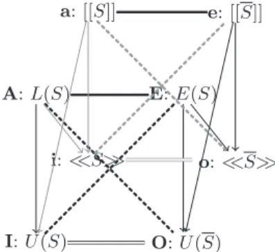
In Figure 7, all these rough set operators are put into the cube. The normal-ization condition on R requires that also R is serial, that is, also in the rough set cube, we have to require that xR is not the entire set of objects X.
i: <<S>> I: U (S) O: U (S) o: <<S>> a: [[S]] A: L(S) E: E(S) e: [[S]]
Fig. 7.Cube of oppositions induced by rough approximations
Remark 1. Often, the operators [[S]] and <<S>> are introduced together with a more general definition of information table. Indeed, it is considered that to each pair attribute-object we can associate more than one value, i.e. we have a many-valued table. For instance, if the attribute a is color with range V ala = {white, green, red, blue, yellow, black}, an object can have both values
{blue, yellow} ⊂ V ala whereas classically each object can assume only a single
value in V ala. In this way, we can define also several forms of generalized
a(x) ∩ a(y) 6= ∅ (in the classical setting, it would be: a(x) = a(y)). Different relations of this kind are considered in [28] both of indistinguishability (based on R) and distinguishability (based on R) type.
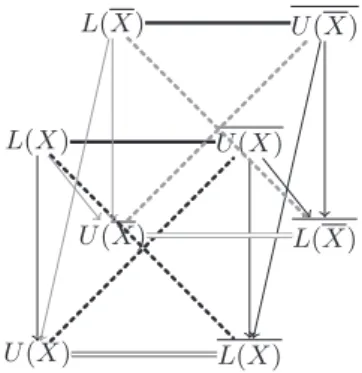
Let us note that the front square of the cube was already defined in [6], but considering only the equivalence relations and all the rest of the cube is a new organization of rough set operators. Indeed, a cube of opposition was also studied in [6] (see Figure 8) but it is of a different kind. In this last case, it is supposed that L and U are not dual, that is L(S) 6= U (S). This is true in some generalized models such as variable precision rough sets (VPRS) [22].VPRS are a generalization of Pawlak rough sets obtained by relaxing the notion of subset.
Indeed, the lower and upper approximations are defined as lα(H) = {y ∈ X :
|H∩[y]|
|[y]| ≥ 1 − α} and uα(H) = {y ∈ X : |H∩[y]|
|[y]| > α}. That is, we admit an error
αin the subsethood relation [y] ⊆ H and if α = 0 we recover classical rough set
approximations. U(X) U(X) L(X) L(X) L(X) L(X) U(X) U(X)
Fig. 8.Cube of opposition induced by generalized approximations
So, an open issue concerns the operators [[]] and <<>> in these generalized contexts. By applying them in variable precision rough sets we can expect to obtain another cube of R approximations and more interesting, it should be investigated if this new setting has some practical application.
3.1 Hexagon
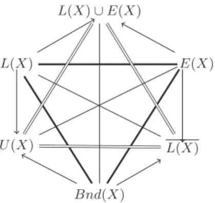
As we have seen, the front face contains the main operators in rough set theory. Also the hexagon, built in the standard way from the front square, is related to rough set operators. This hexagon has been built in [6] and it is reported in Figure 9.
So, on the top we have the set of objects on which we have a clear view: either they belong or not to the set S. On the contrary, on the bottom we have the boundary, that is the collection of unknown objects.
L(X) L(X) ∪ E(X) E(X) L(X) Bnd(X) U(X)
Fig. 9.Hexagon induced by Pawlak approximations
If we consider the back face, then [[S]] ∪ [[S]] is the set of objects which are similar to all objects in the universe, whereas <<S>> ∩ << S >> is the set of objects which are different from at least one object in S and one object in S.
Considering the face AaIi (the face EeOo is handled similarly), which cor-responds to the FCA framework, from the top of the square, one may build
L(S) ∩ [[S]] = {x ∈ X|S ⊆ xR} ∩ {x ∈ X|xR ⊆ S} = {x ∈ X|xR = S} That is, this intersection defines the set of objects which are in relation to all and only the objects in S. So, if R is an equivalence relation, it is either the empty set or the set S. On the contrary, in more general situations (when we have a covering, not a partition), it can be a non-empty subset of S.
With the bottom of the square, we may consider dually
U(S) ∪ <<S>> = {x ∈ X|xR ∩ S 6= ∅} ∪ {x ∈ X|xR ∪ S 6= X}
that corresponds to the set of objects that are in relation with at least one object in S or that are not in relation with at least one object in S.
The counterpart of the hexagon of Fig. 6 makes also sense, and we have L(S) ∪ [[S]] ⊆ U (S) ∩ <<S>>
.
3.2 Other sources of oppositions
Let us notice that up to now we have considered oppositions arising from op-erators L, U, [[]], <<>> definable in rough sets starting from a binary relation R. Other oppositions can be put forward based on other sources. First of all, relations. On the same set of data we can consider several relations besides the standard indiscernibility one, which can be in some kind of opposition among
them. In [6], we have defined a classical square of oppositions based on four rela-tions: equivalence (A), similarity (I), preclusivity (E), discernibility (O). More-over, if we want to aggregate any two of this four relations (for instance, they can represent two agents point of view), we have 16 ways to do it and so we get a tetrahedron of oppositions.
Another source of opposition is given by attributes of an information table. Indeed, they can be characterized as useful or useless with respect to a classifi-cation task. More precisely, Yao in [47], defines a square of opposition classifying attributes as Core (A), Useful (I), NonUseful (E), NonCore (I). The Core con-tains the set of attributes which are in all the reducts3, Useful attributes are those belonging to at least one reduct, NonUseful attributes are in none of the reducts and finally, NonCore attributes are not in at least one reduct.
4
The Cube in Formal Concept Analysis
In formal concept analysis [18], the relation R is defined between a set of objects X and a set of properties Y , and is called a formal context. It represents a data table describing objects in terms of their Boolean properties. In contrast with the data tables mentioned in the previous section on rough sets, we only consider binary attributes here, whose values correspond to the satisfaction or not of properties. As such, no particular constraint is assumed on R, except that it is serial. Indeed, let xR be the set of properties possessed by object x, and Ry is the set of objects having property y. Then, it is generally assumed in practice that xR 6= ∅, i.e. any object x should have at least one property in Y . It is also assumed that xR 6= Y , i.e., no object has all the properties in Y (i.e., xR cannot be empty). This is the bi-normalization of R assumed for avoiding existential import problems in the front and back facets of the cube of oppositions. Similarly, the bi-normalization of Rt means here that no property
holds for all objects, or none object. In other words, the data table has no empty or full line and no empty or full column.
Given a set S ⊆ Y of properties, four remarkable sets of objects can be defined in this setting (corresponding to equations (1)-(4)):
– RΠ(S) = {x ∈ X|xR ∩ S 6= ∅} = ∪
y∈SRy, which is the set of objects having
at least one property in S;
– RN(S) = {x ∈ X|xR ⊆ S} = ∩y6∈SRy, which is the set of objects having no
property outside S;
– R∆(S) = {x ∈ X|xR ⊇ S} = ∩
y∈SRy, which is the set of objects sharing all
properties in S (they may have other ones). – R∇(S) = {x ∈ X|xR ∪ S 6= Y } = ∪
y6∈SRy, which is the set of objects that
are missing at least one property outside S.
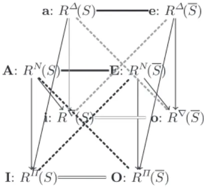
With respect to the notations of the cube of oppositions in Figure 3, we have RΠ(S) = R(S), RN(S) = R(S), R∆(S) = R(S), R∇(S) = R(S). They
3
A reduct is a minimal subset of attributes which generates the same partition as the whole set.
constitute, as already said, four distinct pieces of information. The names given here refer to the four possibility theory set functions Π, N , ∆, and ∇ [9] that are closely related to ideas of non-empty intersection, or of inclusion. The four formal concept analysis operators have been originally introduced in analogy with the four possibility theory set functions [8]. They correspond to the left side facet of the cube of oppositions. The full cube is recovered by introducing the complements, giving birth to the right side facet. Since RΠ(S) = RN(S), and
R∆(S) = R∇(S), the classical square of oppositions AEOI is given by the four
corners RN(S), RN(S), RΠ(S), and RΠ(S), whereas the square of oppositions
aeoion the back of the cube is given by R∆(S), R∆(S), R∇(S), and R∇(S). See
Figure 10. i: R∇ (S) I: RΠ(S) O: RΠ(S) o: R∇ (S) a: R∆(S) A: RN(S) E: RN(S) e: R∆(S)
Fig. 10.Cube of oppositions in formal concept analysis
The counterpart of the hexagon of Figure 6 is given in Figure 11 where all edges are uni-directed, including the diagonal ones, and express inclusions. Indeed, as already directly established [8], under the bi-normalization hypothesis, the following inclusion relation holds: RN(S) ∪ R∆(S) ⊆ RΠ(S) ∩ R∇(S).
In fact, standard formal concept analysis [18] only exploits the third set function R∆. This function is enough for defining a formal concept as a pair made
of its extension T and its intension S such that R∆(S) = T and Rt∆(T ) = S,
where (T, S) ⊆ X × Y . Equivalently, a formal concept is a maximal pair (T, S) in the sense of set inclusion such that T × S ⊆ R. Likewise, it has been recently established [11] that pairs (T, S) such that RN(T ) = S and RtN(T ) = S are
characterizing independent sub-contexts which are such that R ⊆ (T × S) ∪ (T × S). Indeed the two sub-contexts of R contained respectively in T ×S and in T ×S do not share then any object or property. The other connections RΘ(S) = T
and RtΛ(T ) = S where Θ, Λ ∈ {Π, N, ∆, ∇} are worth considering. The cases
Θ = Λ = Π and Θ = Λ = ∇ redefine the formal sub-contexts, and the formal concepts respectively [11], but the other mixed connections with Θ 6= Λ have still to be investigated systematically.
RN(S) RN(S) ∪ R∆(S) R∆(S) R∇ (S) RΠ(S) ∩ R∇ (S) RΠ(S)
Fig. 11.Hexagon induced by the 4 operators underlying formal concept analysis
5
Towards Integrating RST and FCA
In FCA, one starts with an explicit relation between objects and properties, from which one defines formal concepts. This gives birth to a relation between objects (two objects are in relation if they belong together to at least one concept) and similarly to a relation between properties. RST starts with a relation between objects, but with implicitly comes from an information table as in FCA linking objects and attribute values. The classical FCA setting identifies, in the infor-mation table, formal concepts from which association rules can be derived. RST, which is based on the idea of indiscernible sets of objects (note also that in the context of the intent properties, the objects in a formal concept are indiscernible as well), focuses on the ideas of reducts and core for identifying important at-tributes. Besides as we have shown, the structure of the cube of oppositions underlying both RST and FCA provides a richer view of the two frameworks. Thus, for instance, FCA extended with new operators has enabled us to identify independent sub-contexts inside an information table.
In the following, we both provide a synthesis of related works aiming at relating or hybridizing RST and FCA, and indicate various directions for further research taking advantages of the unified view we have introduced in this paper. 5.1 Related Works
Several authors have investigated the possibility of mixing the two theories or finding common points (see [25, 48]), e.g. relating concept lattices and partitions [20], or the place of Galois connections in RST [43], or computing rough concepts [19]. In this section we intend to point out relationships of these works with our approach. Indeed, some of these works are linked to the operators provided by our cubes and to the ideas presented in the previous sections.At first, we consider the works that, more or less explicitly, put forward some of the relations between the two theories that we discussed before. Then, we will give some hint on the
possibility to mix the two theories, this discussion will lead us to the next section about the possibility of integrating RST and FCA.
At first, let us note that Aristotelean oppositions are explicitly mentioned by
Wille in [42]. With the aim of defining a concept logic, he generalizes the idea of formal concept and introduces two kinds of negation, one named weak opposition to model the idea of “contrary”. Given a formal concept (T, S) its opposition is the pair (R∆(S), Rt∆R∆(S)). Clearly, the set R∆(S) is the contrary of the
(standard) extent of R∆(S), as outlined in the FCA cube.
In several studies, it has been pointed out that the basic operators in the two theories are the four modal-like operators of the FCA square of oppositions and that the basic FCA operator is a sufficiency–like operator [12, 13, 48]. This fits well with our setting where it is possible to see that R∆(the sufficiency on FCA)
and [[]] (the sufficiency on RST) are on the same corner of the two cubes. We will better develop this issue in the following section. See also [44] for a modal logic reading of FCA and RST.
Also Pagliani and Chakraborty [29] consider three of the basic operators of the FCA square: RN, RΠ, R∆. Of course, they point out that R∆ is the usual
operator in FCA and moreover they show that in modified versions of FCA, (RΠ(RtN(X)), RtN(X)) is an “object oriented concept” [46] and (RN(RtΠ(X)),
RtΠ(X)) a “property oriented concept” [12]. Further, a generalized upper and
lower approximations are introduced on the set of objects as U (X) = RN(RtΠ(X))
and L(X) = RΠ(RtN(X)). Finally, the special case X = Y is discussed,
provid-ing interpretation of the operators (similarly as we do in Section 3) and showprovid-ing that in case of an equivalence relation, classical rough sets are obtained.
In the attempt at mixing the two theories, several authors considered rough
approximations of concepts in the FCA settings [16, 25, 37, 48]. The basic idea is (see for instance p.205 of [25]) that given any set of objects T , the lower and upper approximations are
LL(T ) = R∆(Rt∆( [ {X|(X, Y ) ∈ L, X ⊆ T )) (6a) UL(T ) = R∆(Rt∆( [ {X|(X, Y ) ∈ L, T ⊆ X)) (6b) where L is the concept lattice of all formal concepts. Clearly, definable sets (i.e., not rough) coincide with the extents of formal concepts.
A different approach to use RST ideas in FCA is given in [27]. Li builds a covering of the universe as the collection R∆({a}) for all attributes a. Then,
he shows that one of the possible upper approximations on coverings (there are more than twenty ones available [49]) is equal to R∆(Rt∆(X)) for all set of objects
X. Once established this equality, rough sets ideas such as reducts are explored in the FCA setting.
In the other direction, that is from FCA to RST, Kang et al. [21] introduce a formal context from the indiscernibility relation of an information table and then re-construct rough sets tools (approximations, reducts, attribute dependencies) using formal concepts.
Finally, the handling of many-valued (or fuzzy) formal contexts has been a motivation for developing rough approximations of concepts [23, 24, 26].
5.2 Some possible directions for the integration of RST and FCA If we try to articulate the FCA cube with the RST one, the necessity of making explicit the role of attributes in the RST case is evident. On its turn this requires to fix a relation. For the moment, let us consider the usual equivalence relation on attributes. As outlined in the previous section, the standard FCA operator R∆ is a sufficiency operator and the corresponding corner of the RST cube is
[[]]. In FCA, R∆(S) is the set of objects sharing all properties in S. In RST, [[]]
is the set of objects which are equivalent to all the objects y ∈ T . Using the attributes point of view: x ∈ [[T ]] iff ∀y ∈ T, ∀a, F (x, a) = F (y, a). So, once fixed a formal concept (T, S) we have that [[T ]]S = R∆(S), where [[]]S means that the
equivalence relation is computed only with respect to attributes in S.
If we do not fix a formal concept then it is not so straightforward to obtain all the formal concepts using rough set constructs. The problem is that the set of attributes used to compute [[T ]]S depends on S which differs from concept
to concept. An idea could be to collect all the equivalence classes generated by all subsets S ⊆ A, as well as all operators [[T ]]S and the ones given by
other corners of the cube. Among all these [[T ]]S (or, it is the same, among all
the equivalence classes) we have all the formal concepts. If among this (huge) collection of operators and equivalence classes, we could pick up exactly the formal concepts then we would have a new common framework for the two theories. In this direction it can be useful to explore the ideas presented in [40], where it is shown that the extents of any formal context are the definable sets on some approximation space.
A different approach in order to obtain formal concepts from rough constructs is to consider the covering made by extents of formal concepts and then consider on it the covering-based rough set lower and upper approximations (as already said more than twenty approximations of this kind are known). Then, we may wonder if any of these rough approximations coincides with the A, I corners of the FCA cube. Let us remark that Li’s approach [27] previously described, is different from this idea, since based on a different covering.
Further, Li’s scope is to use RST constructs such as reducts in FCA. Another issue is to explore the possibility of using the constructs in the FCA cube in order to express the basic notions of RST (besides approximations) such as reducts and cores. We may think that something more is needed, in order to define the notion of “carrying the same information” (at the basis of reducts), where “same information” may mean same equivalence classes, or same covering, or same formal concepts, etc...
The last line of investigation we would like to put forward, is related to ideas directly connected to possibility theory, in particular to a generalization of FCA named approximate formal concept outlined in [11]. Indeed, we may think of such approximate concept as a rough concept, which we want to approximate. Different solutions can be put at work. At first, we can suppose that definable (or exact) concepts coincide with the extent of formal concepts and that any other set of objects should be considered as rough. In this case, we can approximate a rough concept with a pair of formal concepts using equations 6.
On the other hand, given an approximate formal concept (T, S), we may think of it as representing an “approximate set” of objects which share an “ap-proximate set” of properties. So it makes sense to ask which objects in T surely/ possibly have properties in S (and dually, which properties are surely/possibly shared by T ). This means to try to define a pair of lower-upper approximation of the approximate formal concept. For instance, we could consider the pair (R∆(S), R∆,l(S)) where R∆,k(S) is a tolerant version of R∆ admitting up to k
errors. Of course, this framework should be further analyzed and put at work on concrete examples, to understand the potentiality of approximating formal concepts and of their approximations.
6
Conclusion
In this paper, we have shown that both RST and FCA have the same type of underlying structure, namely the one of a cube of oppositions. We have pointed out how having in mind this structure may lead to substantially enlarge the theoretical settings of both RST and FCA. Finally, this has helped us to provide an organized view of the related literature and to suggest new directions worth investigating. In the long range, it is expected, that such a structured view, which also includes possibility theory (and modal logic), may contribute to the foundations of a basic framework for information processing.
References
1. L. Amgoud and H.Prade, A formal concept view of abstract argumentation, Proc. 12th Eur. Conf. Symb. and Quant. Appr. to Reas. with Uncert. (ECSQARU’13), Utrecht, July 8-10 (L. C. van der Gaag, ed.), LNCS 7958, Springer, 2013, pp. 1–12. 2. M. Barbut and B. Montjardet, Ordre et classification: Alg`ebre et combinatoire,
Hachette, 1970, vol. 2, chap.V.
3. J.-Y. B´eziau, New light on the square of oppositions and its nameless corner, Log-ical Investigations 10 (2003), 218–233.
4. R. Blanch´e, Sur l’opposition des concepts, Theoria 19 (1953), 89–130.
5. , Structures intellectuelles. Essai sur l’organisation syst´ematique des con-cepts, Vrin, Paris, 1966.
6. D. Ciucci, D. Dubois, and H. Prade, Oppositions in rough set theory, RSKT Pro-ceedings, Lecture Notes in Computer Science, vol. 7414, 2012, pp. 504–513. 7. , Rough sets, formal concept analysis, and their structures of opposition
(ex-tended abstract), 2013, pp. 4th Rough Set Theory Workshop Dalhousie University, Halifax, Oct. 10 (1 p.).
8. D. Dubois, F. Dupin de Saint-Cyr, and H. Prade, A possibility-theoretic view of formal concept analysis, Fundamenta Informaticae 75 (2007), no. 1-4, 195–213. 9. D. Dubois and H. Prade, Possibility theory: Qualitative and quantitative aspects,
Quantified Representation of Uncertainty and Imprecision (D. M. Gabbay and Ph. Smets, eds.), Handbook of Defeasible Reasoning and Uncertainty Management Systems, vol. 1, Kluwer Acad. Publ., 1998, pp. 169–226.
10. D. Dubois and H. Prade, From Blanch´e’s hexagonal organization of concepts to formal concept analysis and possibility theory, Logica Univers. 6 (2012), 149–169.
11. , Possibility theory and formal concept analysis: Characterizing independent sub-contexts, Fuzzy Sets and Systems 196 (2012), 4–16.
12. I. D¨untsch and G. Gediga, Modal-style operators in qualitative data analysis, Proc. IEEE Int. Conf. on Data Mining, 2002, pp. 155–162.
13. , Approximation operators in qualitative data analysis, Theory and Appli-cations of Relational Structures as Knowledge Instruments, LNCS, vol. 2929, 2003, pp. 214–230.
14. I. D¨untsch and E. Orlowska, Complementary relations: Reduction of decision rules and informational representability, Rough Sets in Knowledge Discovery 1 (L. Polkowski and A. Skowron, eds.), Physica–Verlag, 1998, pp. 99–106.
15. , Beyond modalities: Sufficiency and mixed algebras, Relational Methods for Computer Science Applications (E. Orlowska and A. Szalas, eds.), Physica–Verlag, Springer, 2001, pp. 277–299.
16. B. Ganter and S. O. Kuznetsov, Scale coarsening as feature selection, Formal Con-cept Analysis, Proc. 6th Int. Conf., ICFCA’08, Montreal, Feb. 25-28 (R. Medina and S. A. Obiedkov, eds.), LNCS, vol. 4933, Springer, 2008, pp. 217–228.
17. B. Ganter, G. Stumme, and R. Wille (eds.), Formal Concept Analysis: Foundations and Applications, LNAI, vol. 3626, Springer, 2005.
18. B. Ganter and R. Wille.
19. T. B. Ho, Acquiring concept approximations in the framework of rough concept analysis, Preprint Proc. 7th Eur.-Jap. Conf. Informat. Modelling and Knowledge Bases, Toulouse, May 27-30 (H. Kangassalo and P.-J. Charrel, eds.), 1997, pp. 186– 195.
20. Z.-Z. Li J.-J. Qi, L. Wei, A partitional view of concept lattice, Rough Sets, Fuzzy Sets, Data Mining, and Granular Computing (W. P. Ziarko, ed.), LNCS, vol. 3641, Springer, 2005, pp. 74–83.
21. X. Kang, D. Li, S. Wang, and K. Qu, Rough set model based on formal concept analysis, Information Sciences 222 (2013), 611–625.
22. J.D. Katzberg and W. Ziarko, Variable precision extension of rough sets, Funda-menta Informaticae 27 (1996), no. 2,3, 155–168.
23. R. E. Kent, Rough concept analysis, Rough Sets, Fuzzy Sets and Knowledge Dis-covery (RSKD) (W. P. Ziarko, ed.), Springer, 1994, pp. 248–255.
24. , Rough concept analysis, Fundamenta Informaticae 27 (1996), 169–181. 25. S. O. Kuznetsov and J. Poelmans, Knowledge representation and processing with
formal concept analysis, WIREs Data Mining Knowl Discov, 3 (2013), 200–215. 26. H. Lai and D. Zhang, Concept lattices of fuzzy contexts: Formal concept analysis
vs. rough set theory, Int. J. Approx. Reasoning 50 (2009), no. 5, 695–707. 27. Tong-Jun Li, Knowledge reduction in formal contexts based on covering rough sets,
Proc. Rough Sets and Knowledge Technology, LNCS, 5589, 2009, pp. 128–135. 28. E. Orlowska, Introduction: What you always wanted to know about rough sets,
Incomplete Information: Rough Set Analysis (E. Orlowska, ed.), Physica–Verlag, Springer, Heidelberg, New York, 1998, pp. 1–20.
29. P. Pagliani and M. K. Chakraborty, Formal topology and information systems, Trans. on Rough Sets 6 (2007), 253–297.
30. T. Parsons, The traditional square of opposition, The Stanford Encyclopedia of Philosophy (Fall 2008 Edition) (E. N. Zalta, ed.).
31. Z. Pawlak, Information systems - Theoretical foundations, Information Systems 6 (1981), 205–218.
32. , Rough sets, Int. J. of Computer and Infor. Sci. 11 (1982), 341–356. 33. , Rough Sets. Theoretical Aspects of Reasoning about Data, Kluwer, 1991.
34. Z. Pawlak and A. Skowron, Rough sets and Boolean reasoning, Information Sciences 177(2007), 41–73.
35. , Rough sets: Some extensions, Information Sciences 177 (2007), 28–40. 36. , Rudiments of rough sets, Information Sciences 177 (2007), 3–27. 37. Jamil Saquer and Jitender S. Deogun, Formal rough concept analysis, RSFDGrC,
LNCS, vol. 1711, 1999, pp. 91–99.
38. A. Skowron, J. Komorowski, Z. Pawlak, and L. Polkowski, Rough sets perspective on data and knowledge, Handbook of Data Mining and Knowledge Discovery, Oxford University Press, Inc., 2002, pp. 134–149.
39. R. Slowinski and D. Vanderpooten, A generalized definition of rough approxima-tions based on similarity, IEEE Trans. Knowl. Data Eng. 12 (2000), no. 2, 331–336. 40. P. Wasilewski, Concept lattices vs. approximation spaces, Proc. RSFDGrC, Lecture
Notes in Computer Science, vol. 3641, 2005, pp. 114–123.
41. R. Wille, Restructuring lattice theory: an approach based on hierarchies of concepts, Ordered Sets (I. Rival, ed.), D. Reidel, Dordrecht-Boston, 1982, pp. 445–470. 42. , Boolean concept logic, Conceptual Structures: Logical, Linguistic, and
Computational Issues, Proc. 8th Int. Conf. on Conceptual Structures, ICCS 2000, Darmstadt, Aug. 14-18 (B. Ganter and G. W. Mineau, eds.), LNCS, vol. 1867, Springer, 2000, pp. 317–331.
43. M. Wolski, Galois connections and data analysis, Fund. Infor. 60 (2004), 401–415. 44. , Formal concept analysis and rough set theory from the perspective of finite topological approximations, Trans. Rough Sets III LNCS 3400 (2005), 230–243. 45. Y. Y. Yao, Constructive and algebraic methods of the theory of rough sets, J. of
Information Sciences 109 (1998), 21–47.
46. , A comparative study of formal concept analysis and rough set theory in data analysis, Int. Conf. Rough Sets and Current Trends in Computing, Lecture Notes in Computer Science, vol. 3066, 2004, pp. 59–68.
47. Y. Y. Yao, Duality in rough set theory based on the square of opposition, Funda-menta Informaticae 127 (2013), 49–64.
48. Y. Y. Yao and Y. H. Chen, Rough set approximations in formal concept analysis, T. Rough Sets 4100 (2006), 285–305.
49. Y.y. Yao and B.x. Yao, Covering based rough set approximations, Information Sci-ences 200 (2012), 91–107.