Pépite | Utilisation de la technologie intelligente pour l’optimisation de l’énergie du chauffage dans les bâtiments : développement expérimental et numérique pour la prévision de la température interne

Texte intégral

(1)Thèse de Nivine Attoue, Université de Lille, 2019. PHD Thesis Submitted for the degree of. Doctor of Philosophy Lille University Lebanese University Specialty: Civil Engineering Presented by. ATTOUE Nivine The 13th of May 2019. Use of Smart Technology for heating energy optimization in buildings: Experimental and numerical developments for indoor temperature forecasting. Members of Jury Mr. Hussein Mroueh, Prof., Lille University, France. Director. Mr. Rafic Younes, Prof., Lebanese University, Lebanon. Co-director. Mr. Yacin Fahjan, Prof., Gebze Institute of Technologie, Turkey. Reporter – President. Mrs. Nesserine Ghaddar, Prof., American University of Beirut, Lebanon. Reporter. Mr. Isam Shahrour, Prof., Lille University, France. Member. Mrs. Ariane Abou Chakra, MCF, Insa Toulouse University, France. Member. Mr. Oussama Ibrahim, Prof., Lebanese University, Lebanon. Member. Mrs. Chantale Maatouk, MCF, Saint Joseph University, Lebanon. Member. © 2019 Tous droits réservés.. lilliad.univ-lille.fr.

(2) Thèse de Nivine Attoue, Université de Lille, 2019. Acknowledgement Undertaking this PhD has been a truly life-changing experience, and it would not have been possible to do without the support and guidance that I received from many people.. I would like to express my sincere gratitude to Prof. Isam Shahrour for the continuous support of my PhD study and research, for his patience, motivation, enthusiasm, and immense knowledge.. I would like to acknowledge my supervisors Prof. Hussein Mroueh and Prof. Rafic Younes for their support and encouragement during this thesis.. A very special thanks goes to all jury members: Prof. Yacin Fahjan, Prof. Nesrin Ghaddar, Prof. Oussama Ibrahim, Dr. Ariane Abou Chakra, Dr. Chantale Maatouk and Prof. Fadi Hage Chehadeh for their insightful comments and remarks.. I would like to thank my lab mates and friends for their continued support. Moreover, I am thankful to Dr. Ammar Aljer and Marine Loriot for their collaboration and contribution in the experimental study of this thesis. I am also grateful to Dr. Shaker Zabada and Dr. Ola Hajj Hassan for their valuable guidance. Thanks, are also due to the AUF (Agence universitaire de la francophonie), CNRS – L. (National council for scientific research in Lebanon) and Lille University for their financial support.. I would like to thank my parents Abed El Hadi and Ghada, my sister Lamise and my brothers Ahmad, Bassem and Ali for their endless support and warm love.. Finally, last but no means least, I would like to express my deepest gratitude to my husband Ali and my baby Mohamad. This dissertation would not have been possible without their warm love, continued patience and endless emotional support.. i © 2019 Tous droits réservés.. lilliad.univ-lille.fr.

(3) Thèse de Nivine Attoue, Université de Lille, 2019. Abstract With the highly developing concerns about the future of energy resources, the optimization of energy consumption becomes a must in all sectors. A lot of research was dedicated to buildings regarding that they constitute the highest energy consuming sector mainly because of their heating needs. Technologies have been improved and several methods are proposed for energy consumption optimization. Energy saving procedures can be applied through innovative control and management strategies. The objective of this thesis is to introduce the smart concept in the building system to reduce the energy consumption, as well as to improve comfort conditions and users’ satisfaction. The study aims to develop a model that makes it possible to predict thermal behavior of buildings. The thesis proposes a methodology based on the selection of pertinent input parameters, after a relevance analysis of a large set of input parameters, for the development of a simplified artificial neural network (ANN) model, used for indoor temperature forecasting. This model can be easily used in the optimal regulation of buildings’ energy devices. Results shows that indoor temperature can be well predicted considering only the indoor façade temperature. The smart domain needs an automated process to understand the buildings’ dynamics and to describe its characteristics. Such strategies are well described using reduced thermal models. Thus, the thesis presents a preliminary study for the generation of an automated process to determine short term indoor temperature prediction, heating control and buildings characteristics based on grey-box modeling. This study is based on a methodology capable of finding the most reliable set of data that describes the best the building’s dynamics. The study shows that the most performant order for reduced models is governed by the dynamics of the collected data used. By applying a control approach based on grey box modeling important energy savings were performed. Keywords: Smart technology; artificial neural network (ANN); indoor temperature; façade temperature; forecasting; sensors; grey-box models; performance; input parameters; control.. ii © 2019 Tous droits réservés.. lilliad.univ-lille.fr.

(4) Thèse de Nivine Attoue, Université de Lille, 2019. Résumé L’inquiétude croissante concernant le futur des ressources énergétiques a fait de l’optimisation énergétique une priorité dans tous les secteurs. De nombreux sujets de recherche se sont focalisés sur celui du bâtiment étant le principal consommateur d’énergie, en particulier à cause de ses besoins en chauffage. Les technologies se sont évoluées et plusieurs méthodes sont proposées pour l'optimisation de la consommation d'énergie. L’application des stratégies de contrôle et de gestion innovantes peuvent contribuer à des économies d'énergie. L'objectif de cette thèse est d'introduire le concept intelligent dans les bâtiments pour réduire la consommation d'énergie, ainsi que pour améliorer les conditions de confort et assurer la satisfaction des utilisateurs. L'étude vise à développer un modèle permettant de prédire le comportement thermique des bâtiments. La thèse propose une méthodologie basée sur la sélection des paramètres d'entrée pertinents, après une analyse de pertinence d'un grand nombre de paramètres d'entrée, pour développer un modèle simplifié de réseau de neurones artificiel (ANN), utilisé pour la prévision de température intérieure. Ce modèle peut être facilement utilisé dans la régulation optimale des dispositifs énergétiques des bâtiments. Les résultats indiquent que la température interne peut être prédite en considérant seulement la température interne de la façade. Le domaine intelligent nécessite un processus automatisé pour comprendre la dynamique des bâtiments et décrire ses caractéristiques. L’utilisation des modèles thermiques réduits convient pour de telles stratégies. Ainsi, la thèse présente une étude préliminaire pour la génération d'un processus automatisé pour déterminer la prévision de température intérieure à court terme, le contrôle du chauffage et les caractéristiques des bâtiments basées sur la modélisation en boîte grise. Cette étude est basée sur une méthodologie capable de trouver l'ensemble de données le plus fiable qui décrit le mieux la dynamique du bâtiment. L'étude montre que l'ordre le plus performant pour les modèles réduits est régi par la dynamique des données collectées utilisées. En appliquant une méthode de contrôle basée sur la modélisation en boîte grise, une amélioration de la consommation énergétique a été déduite. Mots-clés : technologie intelligente ; réseau de neurones artificiels (ANN); température intérieure température de façade; prévision; capteurs; modèles en boîte grise; performance; paramètres d'entrée ; contrôle.. iii © 2019 Tous droits réservés.. lilliad.univ-lille.fr.

(5) Thèse de Nivine Attoue, Université de Lille, 2019. Table of contents Acknowledgement .......................................................................................................................... i Abstract .......................................................................................................................................... ii Résumé .......................................................................................................................................... iii Table of contents .......................................................................................................................... iv List of figures ................................................................................................................................ vi List of tables................................................................................................................................... x List of flow charts......................................................................................................................... xi Chapter 0: General introduction ................................................................................................. 1 Chapter 1: State of the Art ........................................................................................................... 3 1.1. Introduction ...................................................................................................................... 3. 1.2. Challenges and motivation ............................................................................................... 3. 1.3. Buildings’ models ............................................................................................................ 7. 1.3.1 Static models................................................................................................................... 8 1.3.2 Dynamic models ........................................................................................................... 10 1.4. Smart technologies ......................................................................................................... 15. 1.4.1 HVAC systems ............................................................................................................. 15 1.5. Conclusion...................................................................................................................... 17. Chapter 2: Experimental developments ................................................................................... 18 2.1. Instrumentation system .................................................................................................. 18. 2.1.1 Design ........................................................................................................................... 18 2.1.2 Sensors .......................................................................................................................... 20 2.1.3 Communication protocol .............................................................................................. 21 2.1.4 Visualization ................................................................................................................. 21 2.2. Study of the occupied office........................................................................................... 22. 2.2.1 Experimental Setup....................................................................................................... 22 2.2.2 Homogeneity of indoor parameters .............................................................................. 23 2.2.3 Usage conditions analysis ............................................................................................. 33 2.3. Study of the four unoccupied class rooms ..................................................................... 35. 2.3.1 Experimental Setup....................................................................................................... 35 2.3.2 Data analysis ................................................................................................................. 36 2.4. Building A4 .................................................................................................................... 39 iv. © 2019 Tous droits réservés.. lilliad.univ-lille.fr.

(6) Thèse de Nivine Attoue, Université de Lille, 2019. 2.4.1 Experimental Setup....................................................................................................... 39 2.4.2 Data analysis ................................................................................................................. 41 2.5. Conclusion...................................................................................................................... 50. Chapter 3: Artificial neural network model ............................................................................. 51 3.1. Bibliographic analysis .................................................................................................... 51. 3.2. Artificial Neural Network approach ............................................................................... 53. 3.3. Prediction time ............................................................................................................... 55. 3.4. ANN models ................................................................................................................... 56. 3.4.1 Facade Indoor Temperature Forecasting – Occupied office ........................................ 56 3.4.2 Facade Indoor Temperature Forecasting – Four unoccupied classrooms .................... 64 3.5. Conclusion...................................................................................................................... 70. Chapter 4: Grey box model ........................................................................................................ 72 4.1. Bibliographic analysis .................................................................................................... 72. 4.2. Grey Box approach......................................................................................................... 74. 4.3. Parameters’ estimation ................................................................................................... 77. 4.3.1 Initialization of parameters ........................................................................................... 78 4.4. Prediction time ............................................................................................................... 80. 4.5. Grey box models ............................................................................................................ 82. 4.5.1 Free Floating data set .................................................................................................... 82 4.5.2 Dynamic data ................................................................................................................ 84 4.6. Sensibility analysis ......................................................................................................... 88. 4.7. Conclusion...................................................................................................................... 91. Chapter 5: Control model .......................................................................................................... 92 5.1. Bibliographic study ........................................................................................................ 92. 5.2. Proposed control methodology....................................................................................... 93. 5.3. Response time determination ......................................................................................... 94. 5.4. Results of the applied control ......................................................................................... 95. 5.5. Other applications ........................................................................................................ 100. 5.6. Conclusion.................................................................................................................... 108. Conclusion and perspective ...................................................................................................... 109 References .................................................................................................................................. 111 Appendix A Publication ........................................................................................................... 119 v © 2019 Tous droits réservés.. lilliad.univ-lille.fr.

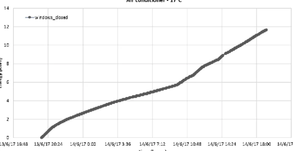
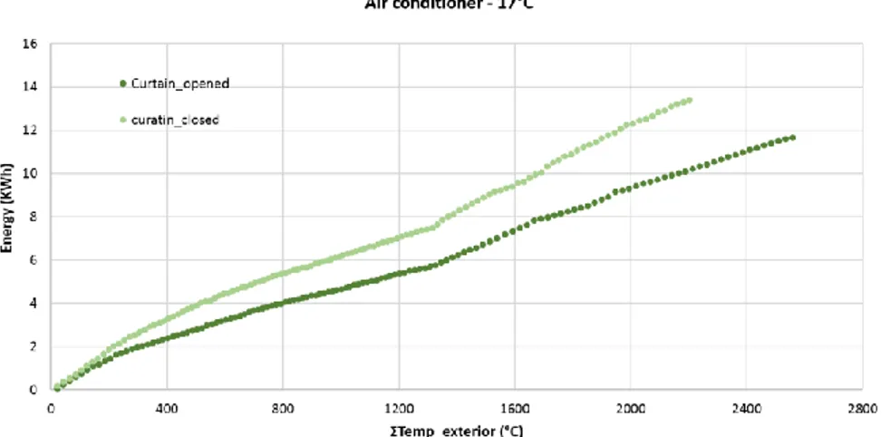
(7) Thèse de Nivine Attoue, Université de Lille, 2019. List of figures Figure 1.1: CO2 emission in France per sector. ............................................................................. 4 Figure 1.2: Final energy consumption per sector. .......................................................................... 4 Figure 1.3: Evolution of energy consumption according to several French regulations. ............... 5 Figure 1.4: Distribution of building energy consumption in France. ............................................. 6 Figure 1.5: Dynamic interaction of building's components. ........................................................... 7 Figure 1.6: Example of building energy signature.......................................................................... 9 Figure 1.7: Different methodologies for dynamic modeling. ....................................................... 10 Figure 1.8: Representation of the black-Box modeling. ............................................................... 12 Figure 1.9: Overview of smart building technologies. ................................................................. 16 Figure 2.1: Architecture of the monitoring system. ...................................................................... 20 Figure 2.2: Central unit. ................................................................................................................ 20 Figure 2.3: Inodesign sensor. ........................................................................................................ 21 Figure 2.4: Example of user’s interface. ....................................................................................... 22 Figure 2.5: Experimented office – First floor. .............................................................................. 22 Figure 2.6: Monitoring plan for the left wall. ............................................................................... 23 Figure 2.7: Recorded data by the sensors located at the same position on the left wall. .............. 25 Figure 2.8: Temperature and relative humidity difference for the sensors located at the same positions. ....................................................................................................................................... 26 Figure 2.9: Temperature variation for wall, facade and air. ......................................................... 26 Figure 2.10: Relative humidity variation for wall, facade and air. ............................................... 27 Figure 2.11: Relative humidity and internal temperature variation. ............................................. 27 Figure 2.12: Temperature variations along the height of the left wall and the center of the room. ....................................................................................................................................................... 29 Figure 2.13: Relative humidity variations along the height of the left wall and the center of the room. ............................................................................................................................................. 30 Figure 2.14: Temperature variations for different distances from the facade............................... 32 Figure 2.15: Relative humidity variations for different distances from the facade. ..................... 33 Figure 2.16: Energy consumption in cases of opened and closed windows with time. ............... 33 Figure 2.17: Energy consumption in cases of opened and closed windows with exterior temperature. .................................................................................................................................. 34 Figure 2.18: Energy consumption in cases of opened and closed curtains with exterior temperature. .................................................................................................................................. 35 Figure 2.19: Experimented rooms – fourth floor. ......................................................................... 36 Figure 2.20: Temperature distribution for different orientation - closed windows. ..................... 36 Figure 2.21: Temperature distribution for different orientation - opened windows. .................... 37 vi © 2019 Tous droits réservés.. lilliad.univ-lille.fr.

(8) Thèse de Nivine Attoue, Université de Lille, 2019. Figure 2.22: Temperature difference for south and north orientation – closed windows. ............ 37 Figure 2.23: Temperature distribution south orientation - closed and opened windows. ............. 38 Figure 2.24: Temperature distribution north orientation - closed and opened windows. ............. 38 Figure 2.25: Temperature difference opened and closed windows – South orientation. .............. 39 Figure 2.26: Temperature difference opened and closed windows – North orientation. .............. 39 Figure 2.27: Instrumentation scheme for building A4. ................................................................. 40 Figure 2.28: Instrumentation plan for the unoccupied room in A4. ............................................. 41 Figure 2.29: Comparison of the temperature at both side of the façade. ...................................... 41 Figure 2.30: Comparison of external façade and window temperatures. ..................................... 42 Figure 2.31: Comparison of internal façade and air temperatures. ............................................... 42 Figure 2.32: Comparison of internal façade and windows temperatures...................................... 43 Figure 2.33: Plan of the sensors installed at the position of the vents. ......................................... 44 Figure 2.34: Daily week variation of temperature for sensors of lines 2 and 5. ........................... 44 Figure 2.35: Daily variation of temperature during the weekend for sensors of lines 2 and 5. .... 45 Figure 2.36: Parameters distribution – day. .................................................................................. 46 Figure 2.37: Parameters distribution – night................................................................................. 47 Figure 2.38: Plan for temperatures’ average distribution: (a) day, (b) night. ............................... 48 Figure 2.39: Plan for temperatures’ minimum distribution: (a) day, (b) night. ............................ 48 Figure 2.40: Plan for temperatures’ maximum distribution: (a) day, (b) night. ........................... 49 Figure 2.41: Air and wall temperatures variation in the open space. ........................................... 49 Figure 2.42: Variation of the temperature inside the open space and the expelled air temperature. ....................................................................................................................................................... 50 Figure 3.1: Schematic diagram of a fully connected multilayer feed-forward neural network. ... 53 Figure 3.2: Façade temperature variation and the air conditioner power. .................................... 55 Figure 3.3: ANN optimal architecture. ......................................................................................... 56 Figure 3.4: Predicted and recorded façade temperatures: (a) Variation of both temperatures in time domain; (b) Predicted façade temperature with the recorded façade temperature. .............. 57 Figure 3.5: R results for different models: (a) Model 1; (b) Model 5; (c) Model 6. ..................... 58 Figures 3.6: Recorded and predicted façade temperature variation in the time domain prediction for 0.5h; (b) prediction for 1h. ...................................................................................................... 60 Figures 3.7: Predicted façade temperature with the recorded façade temperature (Input parameter = Outdoor temperature): (a) prediction for 0.5h; (b) prediction for 1h. ....................................... 60 Figures 3.8: Distribution of the error forecasting (Input parameter = Outdoor temperature): (a) prediction for 0.5h; (b) prediction for 1h. ..................................................................................... 60 Figures 3.9: Recorded and predicted façade temperature variation in the time domain: (a) prediction for 2h; (b) prediction for 4h. ........................................................................................ 61 Figures 3.10: Predicted façade temperature with the recorded façade temperature (Input parameter = Outdoor temperature): (a) prediction for 2h; (b) prediction for 4h. ......................... 62. vii © 2019 Tous droits réservés.. lilliad.univ-lille.fr.

(9) Thèse de Nivine Attoue, Université de Lille, 2019. Figures 3.11: Distribution of error forecasting (Input parameter = Outdoor temperature): (a) prediction for 2h; (b) prediction for 4h. ........................................................................................ 62 Figures 3.12: Distribution of error forecasting (Input parameter = Outdoor temperature and 3h façade temperature): (a) prediction for 2h; (b) prediction for 4h.................................................. 63 Figures 3.13: Predicted and recorded indoor temperatures: (a) Variation of both temperatures in time domain; (b) Predicted indoor temperature with the recorded indoor temperature. .............. 64 Figure 3.14: Distribution of error forecasting for indoor temperature (input parameters = façade temperature). ................................................................................................................................. 64 Figure 3.15: Results of the optimal model for the unoccupied rooms. ......................................... 67 Figure 3.16: R results for different models: (a) Model 4; (b) Model 5. ........................................ 68 Figures 3.17: Distribution of error forecasting (Input parameter = Outdoor temperature and 3h façade temperature): (a) prediction for 0.5h; (b) prediction for 1h. .............................................. 69 Figures 3.18: Distribution of error forecasting (Input parameter = Outdoor temperature and 3h façade temperature): (a) prediction for 2h; (b) prediction for 4h.................................................. 70 Figure 4.1: Thermal model of a building. ..................................................................................... 74 Figure 4.2: RC networks for the four models. .............................................................................. 76 Figure 4.3: Variation of indoor and outdoor temperature while heating. ..................................... 81 Figures 4.4: Error distribution for 15,30 and 60min prediction - Free floating data – order 1. .... 83 Figures 4.5: Error distribution for 15,30 and 60min prediction – Heating 900W- order. ............ 85 Figure 4.6: Residual autocorrelation – heating 900W – order 3. .................................................. 86 Figures 4.7: Error distribution for 15,30 and 60min prediction – Heating 1500W- order 2. ....... 87 Figure 4.8: Residual autocorrelation – heating 1500W – order 2. ................................................ 88 Figure 4.9: Results of sensibility analysis..................................................................................... 90 Figures 5.1: Indoor temperature variation with on/off 1500W heating for order 2 and 3 respectively.. ................................................................................................................................. 74 Figures 5.2: Error temperature variation with on/off 1500W heating for order 2 and 3 respectively ................................................................................................................................... 95 Figure 5.3: Occupation schedule for the studied room for one week of February 2018.. ............ 96 Figure 5.4: Outdoor and comfort temperatures............................................................................. 96 Figures 5.5: Empirical on/off control heating 150W – Model of order2. ..................................... 97 Figures 5.6: Empirical on/off control heating 150W – Model of order3.. .................................... 98 Figures 5.7: Comparison of energy consumption and cost for 24h for different control methods – Model of order 2.. ......................................................................................................................... 99 Figure 5.8: Comparison of energy consumption and cost for 24h for different control methods – Model of order 3.. ....................................................................................................................... 100 Figure 5.9: Modeled offices in building A4................................................................................ 101 Figures 5.10: Indoor temperature variation with on/off 1000W heating for offices 1 and 2.. .... 102 viii © 2019 Tous droits réservés.. lilliad.univ-lille.fr.

(10) Thèse de Nivine Attoue, Université de Lille, 2019. Figures 5.11: Empirical on/off control heating 150W – Model of order3 – Office 1 and 2... .... 103 Figures 5.12: Empirical on/off control heating 150W – Model of order 2 – Office 1 and 2... ... 103 Figures 5.13: Error variation for orders 2 and 3 – Offices 1 and 2.. ........................................... 105 Figures 5.14: Comparison of energy consumption and cost for 24h for different control methods – Model of order 2 – Office 1.. ................................................................................................... 106 Figures 5.15: Comparison of energy consumption and cost for 24h for different control methods – Model of order 3 – Office 1.. ................................................................................................... 106 Figures 5.16: Comparison of energy consumption and cost for 24h for different control methods – Model of order 2 – Office 2.. ................................................................................................... 107 Figures 5.17: Comparison of energy consumption and cost for 24h for different control methods – Model of order 3 – Office 2... .................................................................................................. 108. ix © 2019 Tous droits réservés.. lilliad.univ-lille.fr.

(11) Thèse de Nivine Attoue, Université de Lille, 2019. List of tables Table 1.1: Representation of building thermal factors in an electrical circuit. ............................. 15 Table 3.1: Input parameters for the façade temperature forecasting. ........................................... 56 Table 3.2: Weight of neurons’ connections. ................................................................................. 57 Table 3.3:Analysis of the relevance of input parameters . ............................................................ 58 Table 3.4: Degraded models result. .............................................................................................. 59 Table 3.5: Performances of the forecasting models (Input parameter = Outdoor temperature). .. 61 Table 3.6: Performances of the forecasting models (Input parameters = Outdoor temperature and 3 hours façade temperature). ......................................................................................................... 63 Table 3.7: Input parameters for the façade temperature forecasting. ........................................... 65 Table 3.8: Analysis of the relevance of input parameters. ............................................................ 65 Table 3.9: Performance of different Models for the unoccupied rooms. ...................................... 66 Table 3.10: Degraded models result. ............................................................................................ 68 Table 3.11: Performances of the forecasting models (Input parameters = Outdoor temperature and 3 hours façade temperature). .................................................................................................. 70 Table 4.1: Initial values for the estimated parameters. ................................................................. 77 Table 4.2: Inertia classes for building. .......................................................................................... 79 Table 4.3: Daily capacity. ............................................................................................................. 79 Table 4.4: Conductivity values. .................................................................................................... 79 Table 4.5: Coefficient of internal and external convection........................................................... 80 Table 4.6: 15 min prediction results for the free-floating data. .................................................... 82 Table 4.7: 30 min prediction results for the free-floating data. .................................................... 82 Table 4.8: 60 min prediction results for the free-floating data. .................................................... 83 Table 4.9: 15 min prediction results - heating at 900W................................................................ 84 Table 4.10: 30 min prediction results - heating at 900W.............................................................. 84 Table 4.11: 60 min prediction results - heating at 900W.............................................................. 84 Table 4.12: 15 min prediction results - heating at 1500W............................................................ 86 Table 4.13: 30min prediction results - heating at 1500W............................................................. 86 Table 4.14: 60 min prediction results - heating at 1500W............................................................ 86 Table 4.15: Calculated total Sobol index. ..................................................................................... 89 Table 5.1: Hours classification according to the price of KWh in France 2018. .......................... 93. x © 2019 Tous droits réservés.. lilliad.univ-lille.fr.

(12) Thèse de Nivine Attoue, Université de Lille, 2019. List of flow charts Flow chart 2.1: Different monitored spces and its objective. ....................................................... 15 Flow chart 3.1: Different applied ANN models............................................................................ 56 Flow chart 4.1:Grey box modeling summary. .............................................................................. 77. xi © 2019 Tous droits réservés.. lilliad.univ-lille.fr.

(13) Thèse de Nivine Attoue, Université de Lille, 2019. Chapter 0: General introduction In recent years, energy consumption has been receiving huge public and political attention due to a mix of increasing energy prices, the wish of independence from some energy supplying countries, and last but not least alarming reports about the impacts of CO2 emissions on the global climate. This is while the global energy demand is still increasing - a development expected to continue for years to come due to rapidly growing economies. In industrialized countries, the building sector is one of the biggest consumers of energy whose needs are constantly increasing due to demographic change and the improvement of living’s standards. At present, since the Rio Summit (1992) and the Kyoto Protocol (2005) more attention is being paid to reduce and control energy consumption, which is an economic and environmental necessity. European and particularly French efforts are reflected in the application of various thermal regulations and quality labels. The objective being to play on the building's construction features to reduce energy requirements. The consumed energy in buildings is affected by several factors such as the insulation, the environment and the heating regulation etc.… In order to reduce this consumption, a better understanding of the building performance as well as regulation methods is needed. Static and dynamical relationships are needed for many important purposes such as control of heating and ventilation with respect to indoor comfort. If reliable models of the heat dynamics of buildings can be obtained, the thermal mass in buildings provides an energy storage that may be used to shift some of the energy demand away from demand at peak hours. The design of an environmentally friendly building requires mastery and knowledge of energy and bioclimatic aspects. This implies taking into consideration of all the elements that make up the building and the way in which the energy exchange occurs between these elements. These couplings involve a fundamental reflection to allow an optimal functioning of the building, both in winter and in summer. The study of these energy interactions requires the most often welladapted models. Hence, the Laboratory of Civil Engineering and Geo-Environment (LGCgE) at Lille 1 University and his partners have undertaken a project of great magnitude, that of to build on the campus of Lille 1 university a demonstrator of the smart and durable city (project SunRise). The work of this thesis constitutes a part of this project. The aim of this study is to introduce the smart concept in the building system in order to reduce the energy consumption, as well as to improve comfort conditions and users’ satisfaction. Using smart technologies (sensors) allows following the indoor and outdoor conditions of the building to understand its thermal behavior. The study is applied on tertiary buildings at the school of 1 © 2019 Tous droits réservés.. lilliad.univ-lille.fr.

(14) Thèse de Nivine Attoue, Université de Lille, 2019. engineering ‘Polytech’Lille’ and at the research building “A4” in France. An advanced monitoring system was installed in many buildings for modeling purpose in order to study buildings’ thermal behavior. The objective of the thesis is therefore to develop a model that makes it possible to predict thermal behavior of buildings. The model must be generalizable, and a minimum information should be necessary for its implementation. In addition, it must allow the establishment of energy optimization strategies. In chapter one, we will present increasing energy consumption of buildings and their environmental impact. We focused on the solutions to achieve low energy buildings concerning building regulations and codes. However, this is not enough to achieve the expected goal in 2020. We noted that, improving building performance required a total understanding of their thermal behavior and thus modeling the thermal dynamic system is needed. Different prevision models are identified within a bibliographic analysis.. Chapter two presents a detailed description of the monitoring system installed in Lille 1 university with a deep analysis of the distribution of the measured indoor and outdoor parameters and general conclusions. A set of experimentation with its analysis is described too. This investigation allows the determination of the major factors influencing the indoor temperature for better forecasting and optimization of the heating energy. The next chapter introduces a black box methodology ‘Artificial Neural Network’ and presents a data-based model for indoor and façade temperature forecasting, which could be used for the optimization of energy device use. This study proposed a methodology for the development of a simplified ANN-based model for forecasting indoor temperature. Chapter four describes another grey box methodology to predict the indoor temperature and building characteristics. It presents a study of the influence of the data’s dynamics on the prediction of the indoor temperature. The impact of building’s parameters is determined through a sensitivity analysis. The last chapter presents an empirical on/off control method to minimize the energy consumption. It completes the work of the previous chapter. This study describes the proposed control methodology and analyzes several applications to confirm the effectivity of the control method.. 2 © 2019 Tous droits réservés.. lilliad.univ-lille.fr.

(15) Thèse de Nivine Attoue, Université de Lille, 2019. Chapter 1: State of the Art 1.1 Introduction Energy is the most precious resource among all resources and its demand is rapidly growing. There could be two possible ways to tackle this problem: (1) production of additional energy and exploration of alternate resources and (2) more efficient utilization of existing resources. The first approach is highly expensive, time consuming, and costly, and the second one is inexpensive, more proficient and highly recommended as the efficient utilization of energy avoids the need to produce new energy. Technologies have been improved and several methods are proposed for energy consumption optimization. Energy saving procedures can be applied through innovative control and management strategies. The research issue around the necessity to integrate supply and demand sides has produced important developments, leading to new research purposes based on the system thinking in design and management of buildings. Hence, this thesis concerns the use of the Smart Technology for the optimization of the heating/cooling consumption in buildings. The use of this technology requires forecasting of the indoor temperature for the regulation of energy devices to ensure occupant comfort, as well as for energy optimization. Thus, the use of models for sustainability assessment of intelligent buildings was a key strategy to quantify the improvement of energy efficiency and occupants’ satisfaction. Several models were proposed in this work. In this chapter we will present the challenges of buildings heating/cooling with some data, proposed models for the optimization of the heating consumption, and smart technology for heating optimization.. 1.2 Challenges and motivation In Europe, the energy consumption increases on average by 1.5% per year, due to the economic development, the expansion of the construction sector and energy services used. With a consumption greater than 40% and more than 20% of CO2 emissions (figure 1.1), the building sector is in first position before those of industry and transport [1]. Because of this observation and pushed by its membership, the Kyoto Protocol and by the public will, Europe is now moving towards buildings with very low energy consumption. In France, the French Environment and Energy Management Agency (ADEME) estimated that the building was also the largest consumer of energy in 2015 with 45% of total energy consumed and 25% of Greenhouse Gas emissions (GHG) [2]. In 2015, the Observation and Statistics Service (SOeS), which is part of the General Commission for Sustainable Development always attributed more than 45% energy consumption in the building sector (Figure 1.2) and in contrast to other industrial sectors, emissions from the residential /tertiary sectors and transport continues to grow.. 3 © 2019 Tous droits réservés.. lilliad.univ-lille.fr.

(16) Thèse de Nivine Attoue, Université de Lille, 2019. During the last thirty years, despite the drop of more than a third of the consumption per square meter, consumption increased by almost a quarter [3]. This consumption is based essentially on fossil fuels. Existing buildings account for half of the energy consumption of this sector. Following the Rio Earth Summit in 1992 and the Kyoto Protocol in 1997, France became committed in 2002 to respect the directives of the European Union "Energy Efficiency" with the goal of reducing greenhouse gas emissions. The Climate Plan was launched in 2004, which consists of setting short- and medium-term goals: . Divide by four greenhouse gas emissions by 2050;. . Increase the production of thermal renewable energy by 50% by 2015;. . Increase the production of renewable electricity by 25% by 2015.. Figure 1.1: CO2 emission in France per sector. [2]. Figure 1.2: Final energy consumption per sector. [2]. 4 © 2019 Tous droits réservés.. lilliad.univ-lille.fr.

(17) Thèse de Nivine Attoue, Université de Lille, 2019. Faced with this challenge, the Grenelle Environment Forum set objectives to create favorable conditions to the emergence of a new French deal in favor of the ecology and sustainable development [4]. The High Environmental Quality (HQE) approach was created to meet these objectives and to respect the regulations in the building sector. Following the perspective of 2004 Climate Plan, a passage from the regulation thermal 2000 to 2005 was carried out. RT2005 is applied to all building permits since September 1, 2006 in the residential and tertiary sectors. It strengthens 15% the energy performance requirements of new buildings compared to the RT2000 [4]. To ensure this continuity in improving energy performance, RT2012 has seen then the day. This regulation must be applied to the new residential buildings from the end of 2012 and tertiary buildings from the end of 2010. It increases the level of regulatory requirements to consume less than 50 kWh / m² / year in primary energy (figure 3).. Figure 1.3: Evolution of energy consumption according to several French regulations. [http://www.cfbp.fr/gpl-maitrise-de-lenergie/reglementation-thermique-n261]. Building conception is a principal factor that affects the energy consumption and the comfort in the building. In the European context, this is one of the most important challenges to be worked out. Many facilities were put in action with tools to ameliorate the building energy behavior from the conception phase as mentioned before. However, this is not enough since the rehabilitation of the existing mass of buildings can be very expensive with a very long investment cycle. Moreover, there are other factors that can affect this behavior such as the technical as well as economical and regulatory issues to be integrated.. 5 © 2019 Tous droits réservés.. lilliad.univ-lille.fr.

(18) Thèse de Nivine Attoue, Université de Lille, 2019. Heating and cooling loads represent the largest consumption (more than 60% of total consumption) (figure 1.4) [5] for the building sector. Better management of climatization (heating and cooling) consumption becomes an emergency, especially in a rapidly evolving economy and increased awareness of environmental constraints. Understanding the building heating/ cooling system is challenging as well. The type of the heating/cooling system and its design affects enormously the energy consumption. Buildings with central systems consume totally differently from those with individual systems. The same thing applies for the nature of the heating/cooling system (gas, electricity....). Furthermore, the regulation and planning of the climatization system is highly important and can affect the energy consumption (use of building inertia, occupation planning, sun, energy pricing…).. Figure 1.4: Distribution of building energy consumption in France.. Concretely, it would be a question of choosing a facility well adapted to the needs (management demand for energy) and to ensure that the building is properly insulated, whether existing or under construction. A good knowledge of the thermal behavior of the building (residential, tertiary, industrial) helps to improve the management of the energy demand of heating/cooling system. The marketer uses this information to propose energy service offers such as building diagnosis and recommendations for improving the structure of the building, or replacement of the electric heating system. For the customer, a better knowledge of the behavior of his building is necessary to modify his energetic behavior, to reduce its bill or to improve its comfort. Achieving the energy performance levels already mentioned requires a special attention to the "elements" constituting the building: reducing thermal losses through the envelope, minimizing thermal bridges, choosing a system of ventilation that limits heat loss through air exchange, using phase change, etc. Achieving energy savings is also substituting conventional energy equipment system and strategies with smart ones. Therefore, promoting low-energy buildings requires integration of smart technologies to improve their performance.. 6 © 2019 Tous droits réservés.. lilliad.univ-lille.fr.

(19) Thèse de Nivine Attoue, Université de Lille, 2019. 1.3 Buildings’ models As one of the ways to enhance building energy performance, thermal analyses of building systems should be carried out. The building system includes envelopes of a building and its inner subsystems, such as HVAC and electrical equipment. For obtaining a complete understanding of thermal behavior of a building system, the characteristics of the following components must be known: . Outdoor conditions : orientation, location, climate, etc.. . Physical properties: structure, materials, thermal capacitance, thermal resistance, etc.. . Energy efficiency of inner sub-systems: HVAC, lighting, electrical appliances, renewable energy source installation, etc.. . Occupancy. . Geometry of building. . Window to wall ratio. Figure 1.5: Dynamic interaction of building's components.. These characteristics are dynamically interacting with each other (Figure 1.5). It requires a more detailed study of the above characteristics of the building system to assess its energy performance [6]. In order to obtain a more accurate data, each component of the building system has to be rigorously studied. Furthermore, since the thermal characteristics of the building system are closely related to the energy consumption, thermal modeling of each component of the building system is the most important task to do for analyzing the building energy performance. 7 © 2019 Tous droits réservés.. lilliad.univ-lille.fr.

(20) Thèse de Nivine Attoue, Université de Lille, 2019. Interest in the building as a system that interacts dynamically with a set of climatic data and conditioned by the behavior of the occupant (heat input due to the presence of people, domestic appliances, heating management, etc.) is relatively new. Indeed, the first studies go back to the end of the years 70 and faced three major difficulties: . Lack of detailed information on the constitution of the building.. . Uncertainty about occupant use and behavior.. . Limited capacities of the means of calculation and experimentation of the building.. Two approaches were adopted to model the building. The first was about a simplified modeling to overcome the limitations of the calculation. The proposed models are of a reduced order and the parameters are derived from on-site surveys (electrical power, indoor temperature, etc.). The second was interested in understanding the heat exchange phenomena in the building for simulation purposes. Existing models can be classified into two families according to the adopted approach, a static approach and a dynamic approach. The choice of the method is essentially related to the simplicity of the adopted model and the time interval chosen.. 1.3.1 Static models Static models are dedicated to the modeling of the steady state of the building (the interior temperature is equal to the set point at every moment and the demands are constant in time). This regime results in a thermal balance, ensured at every moment, between foreign exchange (mainly weather) and domestic (heating input parameters) of the envelope of the building. As a result, the static models are designed to express the heating load as a function of the external stresses (for example outside temperature, sunshine, etc.) according to the heat balance equation [7]: 𝑄 = 𝑈 (𝑇𝑖𝑛𝑑 − 𝑇𝑜𝑢𝑡 ) − 𝑆𝐼 + 𝜀. (1.1). where:       . Q is the energy needed to maintain the set temperature; Tind is the average indoor temperature in the building (◦C); Tout is the average outdoor temperature (◦C); U is the coefficient of the global static losses (W/◦C); S is the equivalent south surface (m2); I is the global south vertical radiation (W/m2); ε is a factor that depending on the start and end time of the observation period and it is weighted by the inverse of the measurement time step (W).. 8 © 2019 Tous droits réservés.. lilliad.univ-lille.fr.

(21) Thèse de Nivine Attoue, Université de Lille, 2019. The difference between the proposed models is related to the choice of the number and the assumptions made on the excitations of the studied system. Equation 1.1 can be adapted according to the precision needed and the data available. The term ε can be further developed by taking into consideration more gains to have better precision of calculations. It can be as well further simplified by ignoring ε and even the sun radiation and calculating the heat load as a function of the temperature difference between indoor and outdoor. The most famous application of this concept is the energetic signature (figure 1.6). This method has been designed to analyze heating consumption in the absence of detailed measurements of thermal magnitudes of the building. Here, the goal is to express the heating/cooling load according to the outside temperature. Equation 1.1 can then be simplified in equation 1.2 called building signature. 𝑄 = 𝛼 + 𝛽 𝑇𝑜𝑢𝑡. (1.2). The coefficients α and β can be calculated by linear regression using some registered measures of the studied building.. Figure 1.6: Example of building energy signature.. It can also be interesting to compare buildings in different climatic zones or to evaluate their heating/cooling needs not for a given outside temperature but according to the severity of the climate using the Degree Day concept (DJ). For a given location, the Degree Day is a value representative of the gap between the temperature of a given day and a pre-established temperature threshold (18 or 19°C per example). It is typically used to estimate energy consumption for heating or cooling [9]. 9 © 2019 Tous droits réservés.. lilliad.univ-lille.fr.

(22) Thèse de Nivine Attoue, Université de Lille, 2019. These static models are simple. They offer the possibility of having a first characterization of the building (for the diagnosis for example) through the estimation of its static gain. But they present the three following limitations: . they require a relatively long observation period. . they do not consider the transient behavior of the building. . These models do not make it possible to account for the regulation of heating/cooling.. From where appeared the necessity of dynamic thermal models.. 1.3.2 Dynamic models The transient-state method, called “dynamic” analysis, requires various information and computational calculations in order to provide more detailed and accurate results. This method treats dynamic thermal behavior of building systems, including steady and transient-states. It allows the analysis of temporal and spatial performances within building systems. For example, the gradient of temperature and the diffusion of heat flux inside the building can be described by this method. Furthermore, it is possible to analyze the whole building system that contains the building envelopes and its sub-systems. Given the multitude of methodologies, it is interesting to perform a classification to determine the degree of precision and adaptation of each method. This classification will not be perfect, as the boundary between two levels of modeling is usually not well marked. We will group them into three approaches white box, black box and grey box (figure 1.7).. Figure 2.7: Different methodologies for dynamic modeling.. 10 © 2019 Tous droits réservés.. lilliad.univ-lille.fr.

(23) Thèse de Nivine Attoue, Université de Lille, 2019. 1.3.2.1 White box approach The complete modeling of a building ("white box") allows to predict its thermal needs. This requires a precise knowledge of the composition of walls and measurements [10], which is not always easily accessible. In addition, it is often necessary to group the parts in homogeneous thermal zones, which makes it necessary to take strong assumptions and to have good knowledge of the thermal behavior of the building. Even with such a precise model of the building, the simulated thermal requirements are distance from reality, which makes it necessary to calibrate certain buildings’ parameters to better represent the reality [11]. Once the "white box" model of the building is completed, it is possible to predict the thermal needs of the building by simulation. Moreover, the model will have the possibility to predict the input parameters such as climate data (temperature, sunshine) and occupation profiles. Three main thermal building models are currently used [12]: . CFD ‘Computational fluid dynamics’: Microscopic approach of the thermal transfer model detailing the flow field. It is based on the decomposition of buildings’ zone in many control volumes with global mesh.. . Zonal approach: First degree of simplification of the CFD technique. It consists in dividing each building zone into several cells. One cell corresponds to a small part of a room.. . Multizone or nodal approach: Considers each building zone as a homogeneous volume characterized by uniform state variables approximated to a node that is described by a unique temperature, pressure, concentration, etc.. Even in the most complete models, some phenomena are neglected (for example, the variation in air infiltration rate as a function of external and internal pressures) which can create a bias in load forecasts. Another negative point of the "white box" models is the calculation time. We know that it will be necessary to execute several hundred simulations for the implementation of optimization strategies and this represents an important calculation cost. Physical modeling of the "white box" type is not retained as a solution adapted to the issue of load forecasting and optimization of air conditioning, because it is not generalizable (deployment to many buildings in a short time) and has too important cost of calculation [13, 14]. This method has been applied to several building energy simulation tools, such as DOE-2 [15], HVACSIM+ [16], TRNSYS [17], BLAST [18], and EnergyPlus [19].. 1.3.2.2 Black Box approach Internal operation of the building is not described. This type of model simply allows a numerical resolution of the problem without providing a physical interpretation. The method of resolution is 11 © 2019 Tous droits réservés.. lilliad.univ-lille.fr.

(24) Thèse de Nivine Attoue, Université de Lille, 2019. based on empirical relationships that link the input and output parameters (figure 1.8). These relationships are the result of a regression analysis that requires experimental measurements. In addition, this approach procures a very simple model and accurate results in a reduced calculation time. From existing literature on prediction model where data-driven modelling techniques have been used, it is evident that nonlinear models are more effective than linear models for prediction [2022].. Figure 3.8: Representation of the black-Box modeling.. The simplest building model is linear regression as a function of the outdoor temperature. This static modeling works mainly in heating and on old buildings (few windows, poorly insulated and without temperature reduction). Since the first thermal regulation (RT 88 for non-residential) and following numerous energy savings (Grenelle I & II, Law n ° 2010-788), this case tends to disappear. Rabl [23] shows, on a case study (air-conditioned shopping center), that adding a variable occupancy (in addition to the outside temperature) significantly increases the accuracy of the model. He is one of the first authors to use multiple linear regression to predict the consumption of a building. MISO linear regression models (Multi Input Single Output) are available in several formulations [24]: . ARX model ‘Autoregressive with exogenous input’ where noise is directly coupled to the dynamics of the model. It is efficient if the noise ratio on signal is weak. 𝐴𝑦 = 𝐵𝑢 + 𝑒. . OE ‘Output error’ allows an independent modeling of the dynamic and noise. 𝐵. 𝐴𝑦 = 𝐹 𝑢 + 𝑒 . (1.3). (1.4). ARMAX ‘Autoregressive moving average with exogenous input’, where the dynamics of the model and the noise are coupled, but they may be different for each entry. 𝐴𝑦 = 𝐵𝑢 + 𝐶𝑒. (1.5) 12. © 2019 Tous droits réservés.. lilliad.univ-lille.fr.

(25) Thèse de Nivine Attoue, Université de Lille, 2019. . BJ or ARIMA ‘Box-Jenkins’ or ‘Autoregressive integrated moving average’. Very flexible model, it allows to set independently the dynamics and the noise, whether at input or output. 𝐵. 𝐶. 𝐴𝑦 = 𝐹 𝑢 + 𝐷 𝑒. (1.6). Where y and u are respectively the model output and input, e represents the white noise that consider the unmeasured disturbances in the studied system and A, B, C, D and F are matrices to identify in the learning phase.. Different data-driven non-linear modelling techniques were used by many authors [25-28]. We can mention: . ANN ‘Artificial Neural Network’: Learning technique inspired by the biological neurons used as an approximation tool of the complex relationships between models’ input and output.. . SVM ‘Support Vector Machines’ techniques developed on the concept of decision hyperplanes (nonlinear function). The derived concept is based on finding the largest deviation from the obtained target.. . RF ‘Random Forest’: An ensemble learning methodology where the performance of several weak learners is boosted via a voting scheme.. . GA ‘Genetic algorithm’: Optimization technique deduced from an analogy with the evolution theory of Darwin. It is based on the faculty of a given species to adapt itself to a natural environment and to survive extreme conditions.. Each of these statistical techniques has his own advantages and drawbacks and the choice of the method depends mainly on the user and on what he expects at the end of the study. Black box models ‘data-driven approach’ have shown their limitations as to the need for measurements which require significant resources. Moreover, the optimization study is not based on a physical understanding of the phenomena.. 13 © 2019 Tous droits réservés.. lilliad.univ-lille.fr.

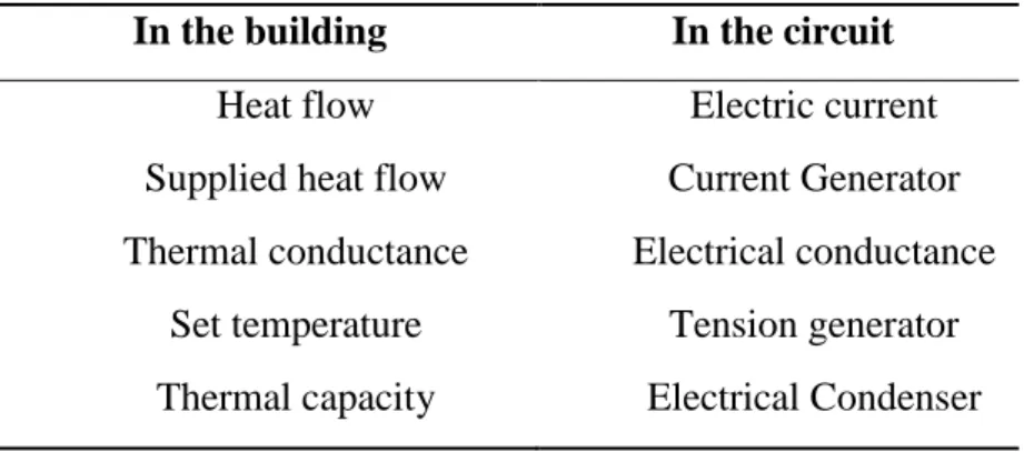
(26) Thèse de Nivine Attoue, Université de Lille, 2019. 1.3.2.3 Grey Box approach Located midway between the black box models and the white box models, the grey box models combine the physical sense and the spirit of simple patterns. The principle of "grey box" modeling is to use a simplified physical representation of the studied system and identify models’ parameters to minimize errors of forecast. Buildings can be modeled by simple dynamic differential equations representing the phenomena of conduction, convection and capacitive phenomena. These equations have been widely studied in the literature, notably by Laret and Roux [29-30]. Indeed, this approach requires computing resources less heavy than those required by white box models and have better flexibility. Its main advantages revolve around the following points:    . Compactness and simplicity of construction of the model given the reduced number of settings; More practical sensitivity analysis; Better flexibility that makes it easy to manipulate the model; Minimization of parameters’ number while keeping an important level of precision.. Several applications are available for this hybrid approach. A first strategy consists in using machine learning techniques (black box) as physical parameters estimator. A second application is to implement a learning model using statistics to describe the building behavior. This learning model is built from a physical approach. A third strategy consists in using statistical method in fields where physical models are not effective and accurate enough. (end uses consideration, heat behavior in multiple zones...) From the mid-1980s, the thermal network method, based on the grey box approach, using the thermal-electrical analogy has been used in order to simplify the building modeling. The thermal network method is based on the energy balance equation. The heat transfer phenomena of building systems are described by their corresponding electrical components. The supplementary heat gain/loss due to solar radiation, metabolic heat of occupants, infiltration/ventilation, and electrical equipment and appliances can be expressed by current sources. It permits the analysis of thermal behavior of building systems during steady and transient-states. Briefly, the thermal models of building systems are represented by electrical circuits, including electrical components and electrical sources. The thermal dynamics of the building systems are analyzed in accordance with the electrical dynamics of the corresponding electric circuits (table 1.1). The choice of the number of resistances and capacities depends on the available data and priorities of modeling process. There are several possible choices according to the use. In the bibliography, models with the forms (RC, R2C2, R3C2, R4C2, ...etc.) were found [31-32]. Some drawbacks own to each technique (white and black box) remain in the hybrid method as the free parameters for statistical tool or the computation time needing for both physical or statistical codes.. 14 © 2019 Tous droits réservés.. lilliad.univ-lille.fr.

(27) Thèse de Nivine Attoue, Université de Lille, 2019. Table 1.1: Representation of building thermal factors in an electrical circuit.. In the building. In the circuit. Heat flow. Electric current. Supplied heat flow. Current Generator. Thermal conductance. Electrical conductance. Set temperature. Tension generator. Thermal capacity. Electrical Condenser. 1.4 Smart technologies Buildings can save energy by using advanced sensors and automated controls in HVAC, plug loads, lighting, and window shading technologies, as well as advanced building automation and data analytics. Buildings that have advanced controls and sensors along with automation, communication, and analytic capabilities are known as smart buildings. In a fully-fledged smart building, the building systems are interconnected using information communications technologies (ICT) to communicate and share information about their operations. Smart building technologies can provide facilities operators with the tools to anticipate and proactively respond to maintenance, comfort, and energy performance issues, resulting in better equipment maintenance, higher occupant satisfaction, and reduced energy consumption and costs. Smart buildings include efficient technologies with automated controls, networked sensors and meters, advanced building automation, data analytics software, energy management and information systems. In the following, we will mention these key building systems and technologies and we will discuss the smart technologies of HVAC systems. Systems that can use smart technologies in buildings are: HVAC systems, plug loads, Lighting, Window shading, Automated system optimization, Human operation and Connected distributed generation and power. Figure 1.9 gives an overview of these interconnected systems. 1.4.1 HVAC systems It takes an enormous amount of energy to condition air and then distribute it throughout a building. Using controls to properly manage HVAC operation is an essential part of saving energy in a building. However, building operators frequently manage HVAC operations through trial-anderror adjustments in reaction to occupant comfort feedback—sometimes relegating energy savings to a much lower priority. Smart HVAC systems have the potential to greatly reduce energy consumption while maintaining or even improving occupant comfort. Smart building software interprets information from a variety of HVAC sensor points and maintains that information in real time, in a cloud-based system that 15 © 2019 Tous droits réservés.. lilliad.univ-lille.fr.

(28) Thèse de Nivine Attoue, Université de Lille, 2019. is remotely accessible. Engineers develop algorithms within the smart building software that use the database information to optimize the monitoring and control of HVAC systems. These advanced controls can limit HVAC consumption in unoccupied building zones, detect and diagnose faults, and reduce HVAC usage during times of peak energy demand. One of the largest energy efficiency benefits of smart building HVAC controls is found through optimizing the amount of conditioned (i.e., heated or cooled) air supplied throughout a building. Although it may seem like a simple concept, this goal can be achieved in several ways. Smart controls can optimize airflow using data provided by occupancy, temperature, humidity, duct static pressure, and air quality sensors. Smart HVAC systems can also support sophisticated data analysis. Armed with smart building data analytics, building operators can review historical building occupancy and usage on a granular level, receive performance data in real time and fine-tune the HVAC controls, accordingly, thereby avoiding wasted HVAC usage.. Figure 4.9: Overview of smart building technologies.. 16 © 2019 Tous droits réservés.. lilliad.univ-lille.fr.

(29) Thèse de Nivine Attoue, Université de Lille, 2019. 1.5 Conclusion This chapter included a state-of-the-art synthesis on the problematic related to buildings energy consumption reduction with a particular focus on models used for the building thermal modelling. Analysis showed that this issue is very complex and still requires effort to build models which could be easily used by professional. The recent development in smart technology offers new opportunity to collect comprehensive data about the building environment and use. These data could be used to build data-based models, which could be easily calibrated and used in indoor temperature forecasting, which constitutes a major step in the optimal thermal management of buildings. In the following chapters we will present the use of this method for the development of two classes of models: Artificial Neural Network model and Grey models.. 17 © 2019 Tous droits réservés.. lilliad.univ-lille.fr.

(30) Thèse de Nivine Attoue, Université de Lille, 2019. Chapter 2: Experimental developments Introduction In this chapter, an intensive and advanced monitoring system will be presented. It was designed to follow the indoor and outdoor conditions of a building. Experimentation were executed at Lille 1 university in the North of France. Monitoring system was installed in three locations at the university campus: an occupied office at the first floor of the school of engineering ‘Polytech’Lille’, four unoccupied classrooms at the fourth floor of the same building and a research building ‘A4’. Furthermore, the chapter presents a preliminary study for each experimentation. It includes a homogeneity investigation of the indoor parameters in order to understand their distribution. Several experimental scenarios were performed to explore the importance of some parameters on the energy consumption. This preliminary analysis is indispensable for the numerical modeling presented in the next chapters. It indicates major parameters that should be considered for heating energy optimization. Flow chart 2.1 presents the planned monitoring of different spaces and its objective. 2.1 Instrumentation system 2.1.1 Design A new monitoring system was designed to study the temperature and relative humidity distributions. Before the design and construction of the system, the determination of its specification was established. This study is a part of the ‘sunrise project’ whose goal was to transform Lille1 university campus into a demonstrator of a smart and durable city. The building monitoring required the design of an innovative monitoring system to follow fluids consumption (water and energy), comfort conditions (temperature, humidity, air quality, lightening, noise) and state of windows and doors (open/closed). The system stores data and allow analysis of historical data. It includes a friendly graphic interface and guarantee tenants’ or researchers’ privacy. The system should also be robust, based on wireless low energy consumption technology and low-cost. The new system is composed of a central unit, wireless sensors and friendly users’ interface (figure 2.1). The central unit with a free and open software communicates with sensors using radio frequency (RF) protocol ensuring the management of the monitoring system. It is formed of a small computer without screen or keyboard, a ‘Raspberry Pi’, which hosts the free and open source Linux operating system for data storage, analysis and display (figure 2.2). A local Wi-Fi network is created by this unit enabling access to stored data and information.. 18 © 2019 Tous droits réservés.. lilliad.univ-lille.fr.

(31) Thèse de Nivine Attoue, Université de Lille, 2019. Monitoring system. Ocuupied office. Applied Study. Applied Study. - Non uniformity distribution of indor parameters. - Most influencing parameters on indoor conditions. - Predicting thermal behavior - Black Box modeling.. Applied Study. -. - Application of different scenarios using air conditioner. Objectives. A4 building. Four unoccupied rooms and classrooms. - Study of th orientation and state of windows parameters.. Objectives. - Most influencing parameters on indoor conditions.. - Predicting thermal behavior Black Box modeling.. Quantitative analysis of indoor parameters. - Qualitative of spacial visualization stdy - GIS.. Objectives. - Indoor parameters disribution. - Predicting thermal behavior - Grey Box modeling.. Flow chart 2.1: Different monitored spaces and its objectives.. 19 © 2019 Tous droits réservés.. lilliad.univ-lille.fr.