Energy-efficient GPS synchronization for wireless nodes

(1)

HAL Id: hal-02968155

https://hal.archives-ouvertes.fr/hal-02968155

Submitted on 16 Oct 2020

HAL is a multi-disciplinary open access

archive for the deposit and dissemination of

sci-entific research documents, whether they are

pub-lished or not. The documents may come from

teaching and research institutions in France or

abroad, or from public or private research centers.

L’archive ouverte pluridisciplinaire HAL, est

destinée au dépôt et à la diffusion de documents

scientifiques de niveau recherche, publiés ou non,

émanant des établissements d’enseignement et de

recherche français ou étrangers, des laboratoires

publics ou privés.

Energy-eﬀicient GPS synchronization for wireless nodes

David Pallier, Vincent Le Cam, Sébastien Pillement

To cite this version:

David Pallier, Vincent Le Cam, Sébastien Pillement. Energy-eﬀicient GPS synchronization for wireless

nodes. IEEE Sensors Journal, Institute of Electrical and Electronics Engineers, 2021, 21 (4), pp.5221

- 5229. �10.1109/JSEN.2020.3031350�. �hal-02968155�

(2)

Energy-efficient GPS synchronization for

wireless nodes

David Pallier, Vincent Le Cam, Sébastien Pillement

Abstract—Synchronization is a challenging problem for wireless nodes, especially for applications demanding good synchronization accuracy over wide areas. In that case, the GPS is a valuable solution as the nodes can independently synchronize to UTC. However, the energy consumption of a GPS receiver (over 100 mW when switched on) is not sustainable on a wireless node. Therefore, in this work, we developed a synchronization scheme based on periodic extinctions of the GPS receiver. The goal is to study the GPS power switching effect on the synchronization accuracy. To do so, a node with dedicated timestamping hardware was designed. Two clock models were compared to predict the node time when the GPS is off and the impact of a Kalman filter, to remove the GPS noise, was evaluated. From experimental data, we show that the choice of the clock model depends on the accuracy needed and that the Kalman filter improves the estimation of the clock frequency for both models. In our design, the GPS can be off from 60% up to 95% of the time for mean synchronization errors of 20 ns to 420 ns, respectively. This work demonstrates that GPS power switching is an efficient solution to reduce energy costs while maintaining a high synchronization accuracy.

Index Terms—Clock synchronization, WSN, Energy efficiency, FPGA, GPS, Kalman filter, Structural Health Monitoring

I. INTRODUCTION

M

ONITORING the health of structures often implies the deployment of many sensor nodes to sample physical parameters such as ambient temperature, constraints, vibra-tions, acoustic waves, electrical fields, etc. Posted to a central supervisor, in delayed or in real-time, those samples are fed to Structural Health Monitoring (SHM) algorithms to assess the infrastructure health. As most of these parameters are time-dependent and sampled from different nodes, the system needs to have a common time reference. The following examples un-derline the need for synchronization and the accuracy needed for SHM applications:

1) The natural frequency range of vibrations for structural diagnostics (modal analysis) is typically comprised be-tween 0 and 100 Hz. Thus, accelerations are usually sampled at 1000 Hz. To ensure good modal reconstruc-tion, the synchronization error between nodes must be lower than 1 ms.

2) Acoustic wave propagation is often used to localize the crack origin in a steel bar or a wire break in bridge cables. The method based on Time Difference Of Arrival (TDOA) is very dependent on the sensor’s ability to timestamp acoustic wavefronts. With a typical velocity of 5000 m/s and a localization accuracy expected to +/-15 cm, synchronization error between two nodes must be lower than 30 microseconds.

3) The TDOA method is also used to monitor the localiza-tion of lightning on high electrical voltage lines. With

This work was supported by the WISE program of Pays-de-la-Loire region

D. Pallier and V. Le Cam, Univ. Gustave Eiffel, Inria, COSYS-SII, I4S, F-44344 Bouguenais, France

S. Pillement, Univ Nantes, CNRS, IETR UMR 6164, F-44000 Nantes, France

a speed of 200 000 km/s and an expected localization of +/- 50 m, synchronization error between two nodes must be under 250 nanoseconds.

Time-counting on an electronic device, such as a wireless node, is mainly based on the use of an oscillator. Unfortu-nately, oscillators are highly sensitive to environmental condi-tions such as temperature, acceleration, or voltage supply sta-bility [1]. Consequently, the frequency of the oscillator drifts from its theoretical value over time. Without a synchronization protocol, each node will have its own local time and the offset between the clocks of the nodes increases over time. In most of the cases, this synchronization protocol relies on timestamps exchange between the nodes. The synchronization accuracy that can be obtained in the network depends on the accuracy of the timestamps exchange, the synchronization update rate, and the stability of local oscillators.

A wireless sensor network (WSN) is a cost-effective way to deploy sensing nodes onto already existing large structures (bridges, wind power plants, railway lines, etc). This is why WSNs are more and more used for SHM applications. How-ever, synchronization between nodes is harder in wireless net-works due to non-deterministic propagation delays. Classical wireless synchronization protocols such as [2], [3] and [4] cannot achieve sub-microsecond accuracy, especially in multi-hop scenarios. In this context the Precision Time Protocol (PTP) has been extended over 802.11 communications with hardware timestamping [5] or synchronization over UWB communications [6] and can achieve sub nanosecond accuracy. While these protocols can offer good synchronization accuracy for the monitoring of small structures, they cannot be used for large structures like bridges, railways or power-lines, as they need close and iterative synchronization process. For large outdoor systems (which are most of SHM applications) a

satel-2 3 4 5 6 7 8 9 10 11 12 13 14 15 16 17 18 19 20 21 22 23 24 25 26 27 28 29 30 31 32 33 34 35 36 37 38 39 40 41 42 43 44 45 46 47 48 49 50 51 52 53 54 55 56 57 58 59

(3)

2 IEEE SENSORS JOURNAL, VOL. XX, NO. XX, XXXX 2017

lite navigation system, like GPS, can be used to synchronize each node to UTC as in [7]. This method is suitable for large infrastructures and allows timestamping accuracy up to tens of nanoseconds. The main limitation of this technique is the energy cost of a GPS receiver. Since energy consumption needs to be minimized in wireless systems, GPS solution needs to be optimized according to the required timestamping accuracy.

In this context, we developed a new synchronization scheme based on GPS holdover. Namely, GPS is used for precision purpose but it will be turned off to save power. During the off-state, the local time of the node is estimated using a clock model. The synchronization accuracy obtained with this scheme depends on the chosen holdover parameters: from tens of ns to 1 ms. To further improve the estimation of the clock model parameters, the GPS signal can be filtered when in on-state. The contributions of this work are: (1) the design of a node with dedicated hardware for timestamping, (2) the accuracy and energy efficiency evaluations of our synchronization scheme for different clock models, and (3) the study of the impact of frequency filtering using a Kalman filter.

The paper is organized as follows. The related works are summarized in Section II. Node architecture, timestamps computation, the use of GPS for periodic re-synchronization and the experimental setup are described in Section III. Section IV introduces the clock models, and the Kalman filter. The results are discussed in Section V, while Section VI resumes our contributions and outlines future perspectives.

II. RELATED WORKS

Since synchronization in distributed systems was first for-malized in [8] and later extended in [9], numerous solutions have been developed to tackle the problem of synchroniza-tion in networks. The Network Time Protocol [10] and the Precision Time Protocol [11] are the most used network syn-chronization protocols over the wired Ethernet. It is possible to obtain microsecond synchronization accuracy with these protocols, and an extension of the PTP [12] aims to achieve sub-nanosecond accuracy.

Classical synchronization protocols for WSNs are based on the exchange of dedicated timestamped RF beacons. These protocols can be divided into two categories: the sender to receiver and the receiver to receiver protocols. In the sender to receiver scheme, a node sends its time to a receiver that timestamp the arrival of the packet using its local time. Then, the receiver synchronizes itself by estimating the offset between its local time and the time of the sender. To estimate the propagation delay a two-way exchange has been developed in [3]. The same principle is used in [4] but on a mesh topology instead of a tree and with the estimation of the packet processing overhead. Other works [13] [14] [15] also rely on the same principle but are optimized for specific nodes with constrained resources like PicoRadios [16]. In the receiver to receiver scheme [2] [17] a third party node broadcast a beacon that doesn’t contain a timestamp. All the receivers timestamp the arrival of the beacon with their local clock

and then exchange their observations pairwise to calculate their offsets. The performances of all these protocols are limited by the propagation delays and the packet processing overhead. The interested reader can refer to [18] that outlines the existing implementations of these techniques and their limitations. While some implementations of these protocols can achieve microsecond accuracy most of them are in the tens of microsecond range. Moreover, the accuracy decreases with the number of hops which can be problematic on large structures such as bridges, railways, or power-lines. Signal processing techniques have been described in [19] to deal with non-deterministic propagation delays but, to the best of our knowledge, these techniques have not been implemented on real wireless nodes.

Other works focus on the implementation of clock syn-chronization in wireless communication norms. ZigBee is the most used protocol in the Low Rate Wireless Area Personal Network (LR WPAN), which adds network and application layers on top of the 802.15.4 protocol. In [20] the Flooding Time Synchronization Protocol (FTSP) is used to synchronize nodes over ZigBee to obtain a timestamping accuracy of 61 µs. The use of UWB for the physical layer was added to IEEE 802.15.4 as an amendment in 2007 and merged in IEEE 802.15.4-2011. In [6] UWB is used to synchronize the clocks of a pair of chips on the same PCB with an accuracy of 374 ps (standard error of 677 ps). Several im-plementations of synchronization protocols over IEEE 802.11 are compared in [21]. IEEE 802.11 compliant synchronization solutions can achieve µs clock synchronization accuracy [22] and non compliant solutions using PTP (IEEE 1588) can achieve nanosecond accuracy [5] or sub-nanosecond accu-racy with a hardware timestamping mechanism. While these synchronization schemes can offer a good synchronization accuracy on small structures, they are not suited for large structures, where the nodes can be distant of a few hundred meters to several kilometers. More recently, Low-Power Wide-Area Network (LPWAN) communications have gained interest for industrial applications. Based on LoRa, Sigfox, or NB-IoT, these protocols allow for communications over a few kilometers in urban areas. In [23] LoRa and NB-Iot are used for node communications in the context of machine vibrations monitoring. Nodes are synchronized every 10 s using LoRa with an accuracy of 5 µs.

Another approach to wireless node synchronization is to use a satellite navigation system, like the GPS, to make each node synchronized to UTC. This solution has been implemented in [7] and [24]. The clock of the node is steered by the PPS signal coming out of its GPS receiver. To achieve an accuracy of tens of nanosecond, dedicated hardware is used with high-speed counters. The use of hardware induces deterministic timestamping which removes software overhead and thus improves the timing accuracy. While this approach is suitable for accurate synchronization, a GPS receiver requires a lot of energy (up to 100 mW). This cost can be affordable for applications requiring a high synchronization accuracy, but for less critical applications that require less accuracy, the energy consumption needs to be optimized. In this work, we propose an adaptive synchronization protocol based on

1 2 3 4 5 6 7 8 9 10 11 12 13 14 15 16 17 18 19 20 21 22 23 24 25 26 27 28 29 30 31 32 33 34 35 36 37 38 39 40 41 42 43 44 45 46 47 48 49 50 51 52 53 54 55 56 57 58 59

(4)

automatic on/off switching of the GPS receiver to minimize the energy consumption under a defined accuracy constraint.

Adaptable synchronization accuracy has already been de-scribed in [17] as an extension of RBS [2]. In [25] a Kalman filter is used to track the offset of a local clock from timestamped message exchange and an algorithm is developed to find the optimal message exchange rate for a parametric accuracy. Our work differs from these solutions as it is designed on top of GPS synchronization (although any GNSS receiver can be used) instead of beacons exchange and relies on dedicated timestamping hardware to achieve up to tens of nanoseconds synchronization accuracy.

III. WIRELESS NODE

A. Node Architecture

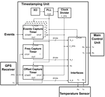
The node design presented in this paper is similar to the one presented in [7]. It includes a dedicated hardware timestamping unit. The timestamping unit is connected to a GPS receiver and has inputs connected to digital signals that have to be timestamped (see Figure 1). The node is synchronized with the PPS signal and the epoch transmitted on a serial link from the GPS receiver. A rising edge on the PPS signal corresponds to the beginning of a UTC second. The epoch corresponds to the number of seconds elapsed since January 6th, 1980. It is used to compute the UTC date at the next rising edge of the PPS signal. The detection of a rising or a falling edge on a digital input of the node is called an event. The events are timestamped with high-speed counters in the timestamping unit and are stored until they are read by the main control unit of the node. This node architecture has several advantages:

• No processing overhead: The use of dedicated hardware on FPGA suppress processing overhead at event detec-tion. Since the delay between the rising edge on the input and the timestamping is deterministic and not affected by software overhead due to process scheduling and interrupt latency, the timestamping accuracy is improved.

• Parallel high granularity timestamping: On most micro-controller units, the number of parallel counters able to timestamp independent events is limited. Another limiting factor is the time granularity fixed by the quartz oscillator frequency. With a custom design, the number of parallel counters is only limited by the FPGA size. The frequency is fixed by the PLL included in the FPGA and can be higher than the quartz oscillator frequency, allowing a higher granularity.

• Asynchronous data fetching and main control unit inde-pendence: Since timestamping and data processing are separated, the main control unit can fetch data (on digital inputs) asynchronously on the timestamping unit. Thus any operating system and any microcontroller can be used as long as the microcontroller is equipped with a serial link.

In this work, we focus on the timestamp unit design. For the main control of the node, without loss of generality and for quick prototyping purposes, we used a Raspberry Pi.

Fig. 1: Timestamp unit

B. Timestamp computation

We define the local estimation of the PPS signal (according to the local quartz oscillator) as the fake PPS signal. The offset θ is then the time between a rising edge of the true PPS signal and the next rising edge of the fake PPS signal (issued by the GPS). It corresponds to the time difference between the local clock and the GPS time. ∆ is the time between a rising edge of the fake PPS signal and a rising edge on a digital input (i.e. an event). θ and ∆ are represented in the timing diagram in Figure 2.

Fig. 2: Timing diagram

The date t[n] of a recorded event occurring during the nth local second is computed based on the date of the true PPS rising edge tpps[n], that occurred during the fake PPS period

and the elapsed time between the event and this rising edge. The elapsed time corresponds to the measured offset θ[n] minus the measured ∆[n] for this particular event. This time is positive when the event is detected after the true PPS edge and negative when detected before. Hence:

t[n] = tpps[n] + θ[n] − ∆[n] (1) 2 3 4 5 6 7 8 9 10 11 12 13 14 15 16 17 18 19 20 21 22 23 24 25 26 27 28 29 30 31 32 33 34 35 36 37 38 39 40 41 42 43 44 45 46 47 48 49 50 51 52 53 54 55 56 57 58 59

(5)

C. Timestamping unit Architecture

The above timlestamp computation is implemented on a Spartan 6 FPGA and is shown in Fig. 1. Since this design aims at turning off the GPS, the clock synchronization is different from the one used in [7]. In this design, the clock counter is not reset by the PPS but instead is bounded by N0. This integer corresponds to the number of clock beats

counted over one second at the nominal frequency f0 of the

quartz oscillator. In the meantime, the local time offset θ is recorded to convert the local timestamp to UTC. The fake PPS signal is generated inside the FPGA, by dividing the local clock frequency to obtain a 1Hz square signal. The offset corresponds to the differential between this signal and the true PPS signal from the GPS receiver. Tracking the local time offset has been chosen over the control of the clock as it allows for both offline and online synchronization. This enables us to perform the timestamp conversion, from local time to UTC, on the fly or post facto if the offset is recorded alongside the events. This post facto synchronization allows us to test different synchronization schemes from the same events dataset for evaluation purposes.

The values θ and ∆ are not directly measured inside the timestamp unit as they are integers corresponding to counter values and not timing values. Let Nθ and N∆be the counter

values corresponding to the offset counter and the event counter, respectively. These integers are converted into time values using the true frequency of the oscillator. Equation 1 becomes:

t[n] = tpps[n] +

1

f [n](Nθ[n] − N∆[n]) (2) With Nf, Nθ and N∆the counter values from the timestamp

unit, while tpps is obtained from the GPS receiver.

The number of local clock beats counted during a full period of the true PPS signal is Nf. Let TGP S be the time elapsed

between two rising edges of the true PPS signal. If the true PPS signal is perfect then TGP S is one second. The true frequency

of the local oscillator can be computed as follows:

f [n] = Nf[n] TGP S[n] (3) giving: t[n] = tpps[n] + TGP S Nf[n] (Nθ[n] − N∆[n]) (4)

If the true PPS signal is perfect, the only residual error is due to the granularity resolution as Nf, Nθand N∆are integer

values. The frequency output of the PLL inside the FPGA was set to 240MHz giving a counter resolution of 4.17 ns.

D. Periodic re-synchronization from GPS

As described in [26], GPS synchronization allows for a timing accuracy under 60ns. However, it entails a substantial energy cost as the GPS receiver is constantly on. When a lower accuracy is needed, GPS can be used periodically to re-synchronize the node. Between two synchronizations, the GPS receiver is off to save energy. The accuracy that can be obtained depends on the re-synchronization period. To be able

to deliver the PPS and the epoch, the GPS receiver needs to decode parts of the navigation message broadcasted by the GPS satellites. In normal conditions the GPS receiver has to: • Generate PPS: In order to generate the PPS signal, the GPS receiver needs to track the "in-view" satellites, compute its time and position (called fix) and then lock its clock. According to [26] the time to first fix is under 1 second when the ephemeris are still valid. From experimentations, we observed less than 1 second to get a fix and less than 4 seconds to lock the clock.

• Refresh ephemeris: In order to track the in-view satellites the receiver needs to compute its position, therefore the ephemeris needs to be updated. In this work, we update them at their typical update rate of two hours.

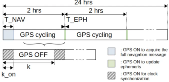
• Acquire a complete navigation message: Since the ephemeris are already acquired every two hours the complete navigation message is acquired once a day. In between the above phases, we propose to turn on and off the GPS to save energy. The off phase is called holdover and correspond to the time between two consecutive GPS time synchronizations. Figure 3 shows the on and off phases of the GPS receiver for a 24 hours period. The T_NAV is 25 minutes long every 24 hours. The T_EPH is 1 minute long every 2 hours. The GPS is on during kon seconds and in holdover

during k − kon seconds. In this mode, the GPS receiver

is switched off (except its memory to keep the ephemeris). Equation 5 gives r, which represents the on/off ratio of the GPS receiver over 24 hours as a function of the parameters k, kon, TN AV and TEHP. r = TN AV + 1 86400.(kon. 7200 − TN AV k + 11.kon. 7200 − TEP H k ) (5)

The minimum konis 5 seconds to get at least one locked pulse

on the PPS signal, after this first delay the receiver delivers one pulse per second. Two pulses are required to get Nθ, N∆

and Nf. The main difficulty is then to track the offset of the

fake PPS, while the GPS is in holdover mode.

Fig. 3: Synchronization process from GPS

IV. OFFSET TRACKING

A. Clock model

The offset needs to be predicted during the holdover to have accurate timestamping. To do so a clock model is used. Let

1 2 3 4 5 6 7 8 9 10 11 12 13 14 15 16 17 18 19 20 21 22 23 24 25 26 27 28 29 30 31 32 33 34 35 36 37 38 39 40 41 42 43 44 45 46 47 48 49 50 51 52 53 54 55 56 57 58 59

(6)

C(t) be the node local time as a function of the real time. C(t) =

Z t

0

ω(τ )dτ + θ0 (6)

With ω the clock rate and θ0the offset at the origin. A perfect

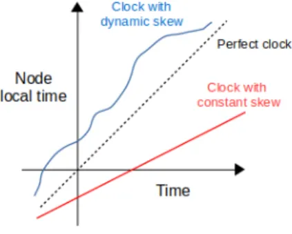
clock would yield C(t) = t. The C(t) = ω.t + θ model is often used [2] [4]. In this model, the clock rate is constant but not equal to one. This is due to the fact that most of the oscillators are not functioning at their nominal frequency, but at a frequency supposed to be constant. While the latter is known to be false for crystal quartz oscillator, the variations of the frequency over a short time can be small enough to be considered constant since ambient temperature moves slowly. Fig. 4 represents the local time as a function of the real time for a perfect clock, a clock with a constant rate and a clock with a varying rate. The oscillator used in this design is an SPXO with an overall frequency stability of +/-20 ppm. Typically, the frequency stability of these oscillators is in the ppb range for sampling intervals of one second [21].

Fig. 4: Constant and dynamic skew of the local time over UTC The offset of a clock at time t is the difference between its local time C(t) and the real time t. Thus the local time offset θ(t) can be expressed as:

θ(t) = C(t) − t (7)

= Z t

0

ω(τ )dτ + θ0− t (8)

Since the offset is sampled every second in the node, a discrete time model is needed. Equation 8 becomes:

θ[n] = n X i=1 ω[i].τ [i] − n X i=1 τ [i] + θ0 (9)

With τ representing the duration of a supposed second for the node. This duration depends on the frequency of the node’s oscillator and can be expressed as:

τ [n] = N0 f [n] =

N0

Nf[n]

.TGP S[n] (10)

The clock rate ω[n] can be computed from the number of local clock beats counted during TGP S[n]:

ω[n] = Nf[n] N0 (11) Therefore: θ[n] = n X i=1 TGP S[i] − n X i=1 τ [i] + θ0 (12)

If the PPS is considered perfectly synchronized to UTC, TGP S= 1s and thus: θ[n] = n − n X i=1 N0 Nf[i] + θ0 (13)

In holdover mode, τ is not known since the GPS receiver is off. The simplest method to estimate it is to use its last value that was observed when the GPS was on. Since the error on the offset is the sum of the error on τ , this error will grow as τ drift away from its last observed value. In that case, the synchronization accuracy will depend on the holdover time and the drift rate of τ . This model will now be referred to as the Constant Skew Clock Model (CSCM).

Another model, that will be referred to as the Linear Skew Clock Model (LSCM), is to consider that τ is evolving linearly during the holdover mainly due to slow variations of the ambient temperature. In this model, the clock skew is considered as dynamic (see Fig. 4) and approximated by a piecewise linear function. The clock skew can be computed as:

τ [n + 1] = τ [n] + u (14) with u the common difference that can be evaluated for every holdover as:

u = τ [n] − τ [n − k]

k (15)

Under the hypothesis that u changes slowly, the last seen u can be used to predict τ during the holdover.

B. Kalman filter

In the previous section, the PPS signal was considered as perfect. In reality, this signal from the GPS receiver is subject to jitter, which creates noise in the frequency and offset measurement. According to [26], the RMS of the timing accuracy is 30ns. While this noise can be neglected when the GPS receiver is always on, it is not the case in the holdover mode. Indeed, the absolute offset error is the sum of the offset errors over time. The offset error growth, during holdover, depends on the accuracy of the measured frequency of the local oscillator at the beginning of the holdover.

To filter the noise on the PPS signal when the GPS is on, a Kalman filter was implemented. This filter uses the good short term accuracy of the local clock to filter the noisy PPS observations. The behavior of the fake PPS period τ during the short GPS on-time period is modeled by a random walk process:

τ [n + 1] = τ [n] + v[n] with v[n] ∼ N (0, σv2) (16)

Let z be the observations of τ from the noisy PPS signal: z[n] = τ [n] + w[n] with w[n] ∼ N (0, σ2_w) (17) The Kalman filtering process is based on the classical follow-ing equations [27]: 2 3 4 5 6 7 8 9 10 11 12 13 14 15 16 17 18 19 20 21 22 23 24 25 26 27 28 29 30 31 32 33 34 35 36 37 38 39 40 41 42 43 44 45 46 47 48 49 50 51 52 53 54 55 56 57 58 59

(7)

With q = σv2 and r = σw2. This filter is stable [28]. The state

variable is initialized with the observation. The variables r, q and p0 are chosen empirically.

V. RESULTS AND DISCUSSION

To evaluate the synchronization algorithms detailed in the previous section, an experimental setup has been developed. Two wireless nodes based on the architecture detailed in section III were implemented on raspberry pis and spartan 6 development boards with their digital inputs connected to the same output of a low-frequency signal generator. This generator generates rising edges (i.e. events) every 2.34 sec that are timestamped by the nodes.

The nodes were placed indoor and the GPS antennas on the roof of the building. The fixed mode was used on the GPS receivers [26]. This GPS configuration is available on certain timing receivers from Ublox. It allows the user to define the GPS antenna location in the receiver to enhance the local time estimation and thus deliver a better PPS signal. The nodes recorded events during more than 2 days. Over 2 × 105_{frequency and offset samples were recorded for each}

node as well as up to 8.5 × 104 _{event samples.}

A. Clock models comparison

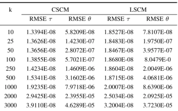
First, we compared the clock models. In Fig. 5 the estimated τ with the CSCM and the LSCM are plotted against the observed τ on a part of the dataset and for k = 1000s. The LSCM seems to be closer to the observations than the CSCM. However, Figure 6, which shows the same variables on another part of the dataset, the CSCM seems closer to the observations. The RMSE of the LSCM and the CSCM for the estimation of τ and θ on the full dataset and for k ranging from 10 to 3000, are summarized in Table I. The RMSE for τ and θ were computed on the difference between the predicted τ and θ and the GPS observations.

We can see from this Table that the LSCM outperforms the CSCM for both τ and θ, when k > 1000. The PPS noise explained in Subsection IV-B can be seen in the observations in both figures. The fact that the LSCM yields poorer results than the CSCM for k _{6 1000 is most probably due to this} PPS noise.

Fig. 5: Observed and predicted τ on the first part of dataset

Fig. 6: Observed and predicted τ on the second part of dataset

B. Impact of the Kalman filter

The impact of the Kalman filter on the offset tracking performance was evaluated. As seen in Section IV-B the Kalman filter is only used when the GPS is "on" to filter the PPS noise. Since the performance of the filter depends on the "on" mode duration, the effect of this duration was studied. To do so we ran the Kalman filter for different kon

and for different k. Then the on/off ratio r was calculated according to Eq. 5. Figure 7 shows the r against the RMSE of the offset for different values of kon. The RMSE increases

as the ratio decrease since a longer holdover yields a poorer synchronization accuracy but a better ratio. From these results

TABLE I: RMSE of the CSCM and LSCM

k CSCM LSCM

RMSE τ RMSE θ RMSE τ RMSE θ

10 1.3394E-08 5.8209E-08 1.8527E-08 7.8107E-08 25 1.3626E-08 1.4230E-07 1.8483E-08 1.9750E-07 50 1.3656E-08 2.8072E-07 1.8467E-08 3.9577E-07 100 1.3855E-08 5.7021E-07 1.8680E-08 8.0479E-0 250 1.4234E-08 1.4609E-06 1.8604E-08 2.0049E-06 500 1.5341E-08 3.1602E-06 1.8715E-08 4.0681E-06 1000 1.9235E-08 7.9718E-06 2.0007E-08 8.6390E-06 2000 2.9425E-08 2.3955E-05 2.5034E-08 2.0925E-05 3000 3.9110E-08 4.6289E-05 3.2004E-08 3.7230E-05

1 2 3 4 5 6 7 8 9 10 11 12 13 14 15 16 17 18 19 20 21 22 23 24 25 26 27 28 29 30 31 32 33 34 35 36 37 38 39 40 41 42 43 44 45 46 47 48 49 50 51 52 53 54 55 56 57 58 59

(8)

we chose kon = 5 seconds since it seems to be the optimal

duration for a RMSE ranging from 10ns to 50 µs. A lower kon slightly improves the ratio for longer holdover but worsen

it for shorter ones.

Fig. 7: Optimal kon depending on the ratio r

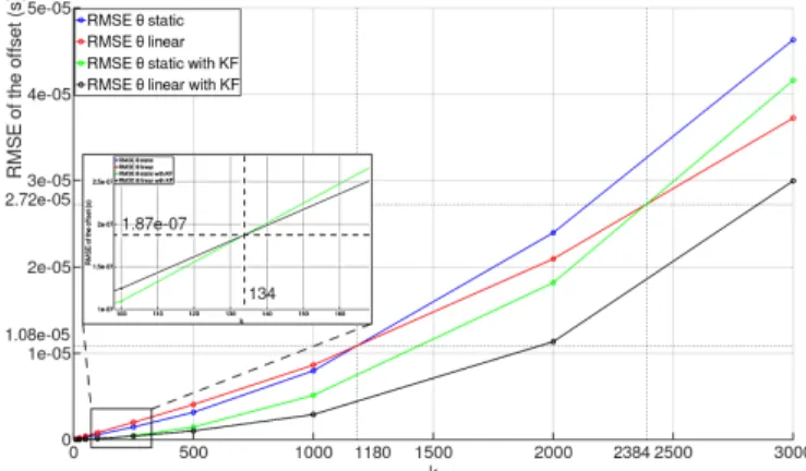
Figure 8 shows τ for k = 1000s and for the same part of the dataset than in Fig. 6. As can be seen the filtered LSCM seems to fit the observations better than the CSCM. Fig. 9 shows a comparison of the filtered and non-filtered models. The RMSE of the offset is plotted against k. It can be seen that both models can be used for the filtered and non-filtered cases depending on the holdover duration. It can also be seen that the Kalman Filter models yield better results than the non-filtered models. For a holdover duration of less than 134s, the filtered CSCM produces better results, for a holdover duration over 134s the hypothesis of a slowing changing u seems valid and the filtered LSCM yields better results.

Fig. 8: Observed and predicted τ using a Kalman filter

C. Timestamps

Then we compared the timestamping errors between the different models. The timestamps are computed according to Eq. 2. The timestamp errors are the differences between the timestamps computed with the GPS always "on" and the timestamps computed with the periodic GPS extinctions. Fig. 10 shows the RMSE of the timestamps errors as a function of k for both nodes. As expected the filtered CSCM yields

Fig. 9: Offset RMSE for the different models

the best results for holdover up to around k = 200s while the filtered LSCM produces best results above. The evolution of the RMSE as a function of the holdover is approximately the same for both nodes.

Finally, we computed the GPS "on"/"off" ratio for all the models. These ratios are plotted against the RMSE on a semi-log scale, in Fig. 11. It can be seen that for all models the ratio decreases exponentially as the RMSE increases and that they all converge to the limit of 2.5%. This limit corresponds to the minimal GPS ratio according to Eq. 5. The Kalman filter improves the ratio by a factor 3 under the microsecond accuracy despite a longer "on" state. The filtered CSCM yields a maximum improvement of 7% on the ratio over the filtered LSCM under 200s and the gain of the filtered LSCM above is marginal (0.5% max) as it happens for a RMSE greater than 300 ns. The results are similar for both nodes.

Fig. 10: Timestamps RMSE on both nodes

D. Discussion

Our synchronization solution allows for a RMSE under 10 ns with the GPS always "on". The RMSE stays under 20 ns on both nodes with a GPS "off" 60% of the time. For a GPS "off" 80% of the time and 95% of the time, the RMSEs are under 50 ns and 420 ns, respectively. As the computations were conducted offline (i.e a posteriori) to test different models, the GPS receiver was only virtually off but our study showed that the GPS receiver energy consumption could be divided

2 3 4 5 6 7 8 9 10 11 12 13 14 15 16 17 18 19 20 21 22 23 24 25 26 27 28 29 30 31 32 33 34 35 36 37 38 39 40 41 42 43 44 45 46 47 48 49 50 51 52 53 54 55 56 57 58 59

(9)

Fig. 11: GPS ratio as a function of timestamps RMSE

by a factor 20 with a mean synchronization error of half a microsecond when implemented with real-time GPS cycling.

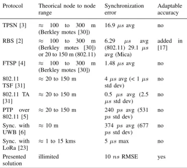
However, the data showed that the distribution of the times-tamps errors is not exactly normal as it has heavy tails. It was observed that the absolute maximum error is approximately ten times bigger than the RMSE for all our experiments. But even with an accuracy limit ten times bigger than the RMSE, the GPS can be switched off 60% of the time for a maximum error under 200 ns or 95% of the time for a maximum error under 4.2 µs. Table II summarizes the node to node theoretical range and the accuracy of existing synchronization protocols. TPSN, RBS, or FTSP with Berkley motes can offer µs synchronization accuracy on small networks with low complexity hardware. Standard IEEE 802.11 synchronization protocols offer the same synchronization accuracy, but sub-nanosecond accuracy can be obtained with the use of PTP. However, the range is still limited to local networks. Sub-nanosecond accuracy can also be obtained with UWB for an even smaller range. For long-range and wide networks, LoRa has been used to obtain 5 µs accuracy with synchronization updates every 10s. In comparison, the presented GPS based solution has a maximum accuracy of 10 ns (RMSE) and an accuracy of 4.2 µs for synchronization updates every 100 s.

While dedicated hardware is important for multiple channel high accuracy timestamping, the spartan 6 development board used in this work is not the best target to implement the design as it draws almost as much current as the GPS receiver. But it is only a proof of concept and the timestamp unit can be implemented on a dedicated ASIC or a smaller FPGA or a CPLD. We already implemented this unit on a smaller FPGA (lattice ICE40 [29]) with a slightly lower resolution for a power consumption of 35 mW. For comparison, the ublox receiver needs 150mW when fully ON and the active GPS antenna draws another 10 to 60 mW (depending on the antenna used).

VI. CONCLUDING REMARKS

Synchronization is a challenging problem for wireless nodes, especially for applications requiring good timestamping accuracy across wide areas. Taking into consideration these applications we designed a node with a simple timestamping

Protocol Theorical node to node range Synchronization error Adaptable accuracy TPSN [3] ≈ 100 to 300 m (Berkley motes [30]) 16.9 µs avg no RBS [2] ≈ 100 to 300 m (Berkley motes [30]) or 20 to 150 m (802.11) 6.29 µs avg (802.11) 29.1 µs avg (Mica) added in [17] FTSP [4] ≈ 100 to 300 m (Berkley motes [30]) 1.48 µs avg no 802.11 TSF [31] ≈ 20 to 150 m 4 µs avg (< 1 µs std dev) no 802.11 TA [31] ≈ 20 to 150 m 0.5 µs avg (2.5 µs std dev) no PTP over 802.11 [5] ≈ 20 to 150 m 240 ps avg (531 ps std dev) no Sync. with UWB [6] ≈ 10 m 374 ps avg (677 ps std dev) no Sync. with LoRa [23] ≈ 1 to 15 kms 5 µs max no Presented solution

illimited 10 ns RMSE yes

TABLE II: Range and accuracy of synchronization protocols

dedicated hardware that uses GPS for synchronization. In order to adapt the energy cost of the GPS receiver to the times-tamping accuracy needed by the applications, we developed a synchronization scheme based on periodic GPS extinction.

We found that both proposed models can be used depend-ing on the timestampdepend-ing accuracy needed. For a timestamp RMSE shorter than 300 ns, the constant skew model shows longer holdovers and for a RMSE above the 300ns, the linear model shows longer holdovers. However, it was shown that since most of the GPS ratio gains occur before 300 ns, the linear model yields minor improvements in terms of energy consumption. As expected the use of a Kalman filter to reduce the GPS noise improves the estimation of the local oscillator frequency and thus allows for longer holdover. But we also showed that this holdover length gain compensates for the longer required "on" state duration and overall the filtered models yield better GPS "on"/"off" ratios. We demonstrated that our solution can significantly reduce the energy cost of the GPS receiver depending on the required synchronization accuracy.

In future works, "online" implementations of our solution will be studied to evaluate the gains in energy consumption. Another interesting direction will be the automatic interrup-tion of the holdover according to ambient temperature mea-surements. This could improve our synchronization scheme, especially for long holdovers, since it was observed that quick temperatures changes can lower the prediction accuracy. Fi-nally, the use of time to digital converters will be investigated as it could allow us to lower the clock frequency inside the FPGA while maintaining, or even improving, the granularity.

REFERENCES

[1] J. R. Vig, “Introduction to quartz frequency standards,” U.S. Army Electronics Technology and Devices Lab., NJ, USA, SLCET-TR-92-1, Tech. Rep., 1992.

1 2 3 4 5 6 7 8 9 10 11 12 13 14 15 16 17 18 19 20 21 22 23 24 25 26 27 28 29 30 31 32 33 34 35 36 37 38 39 40 41 42 43 44 45 46 47 48 49 50 51 52 53 54 55 56 57 58 59

(10)

[2] J. Elson, L. Girod, and D. Estrin, “Fine-grained network time synchronization using reference broadcasts,” ACM SIGOPS Operating Systems Review, vol. 36, pp. 147– 163, Dec. 2002, 10.1145/844128.844143.

[3] S. Ganeriwal, R. Kumar, and M. B. Srivastava, “Timing-sync protocol for sensor networks,” in Proc. SenSys, Los Angeles, CA, USA, Nov. 2003, pp. 138–149.

[4] M. Maróti, B. Kusy, G. Simon, and A. Lédeczi, “The flooding time synchronization protocol,” in Proc. SenSys, New York, NY, USA, Nov. 2004, pp. 39–49.

[5] R. Exel, “Clock synchronization in ieee 802.11 wireless lans using physical layer timestamps,” in IEEE Int. Symp. on Precision Clock Synchronization, San Francisco, CA, USA, Sep. 2012, pp. 1–6.

[6] T. Beluch, D. Dragomirescu, and R. Plana, “A sub-nanosecond synchronized mac–phy cross-layer design for wireless sensor networks,” Elsevier Ad hoc net-works, vol. 11, no. 3, pp. 833–845, Oct. 2012, https://doi.org/10.1016/j.adhoc.2012.09.010.

[7] V. Le Cam, M. Döhler, M. Le Pen, I. Guéguen, and L. Mevel, “Embedded subspace-based modal analysis and uncertainty quantification on wireless sensor plat-form pegase,” in EWSHM, Spain, Jul. 2016, pp. 1705– 1715.

[8] L. Lamport, “Time, clocks, and the ordering of events in a distributed system,” Commun. ACM, vol. 21, no. 7, pp. 558–565, Jul. 1978, 10.1145/359545.359563.

[9] T. Srikanth and S. Toueg, “Optimal clock synchroniza-tion,” J. ACM, vol. 34, no. 3, pp. 626–645, Jul. 1987, 10.1145/28869.28876.

[10] D. L. Mills, “Internet time synchronization: the network time protocol,” IEEE Trans. Commun., vol. 39, no. 10, pp. 1482–1493, Oct. 1991, 10.1109/26.103043.

[11] K. B. Lee and J. Eldson, “Standard for a precision clock synchronization protocol for networked measurement and control systems,” in 2004 Conf. IEEE 1588, Standard for a Precision Clock Synchronization Protocol for Net-worked Measurement and Control Systems, 2004. [12] J. Serrano, M. Lipinski, T. Wlostowski, E. Gousiou,

E. van der Bij, M. Cattin, and G. Daniluk, “The white rabbit project,” 2013.

[13] J. Van Greunen and J. Rabaey, “Lightweight time syn-chronization for sensor networks,” in Proc. ACM WSNA, San Diego, CA, USA, Sep. 2003, pp. 11–19.

[14] K. Römer, “Time synchronization in ad hoc networks,” in MobiHoc, CA, USA, Oct. 2001, pp. 173–182. [15] M. L. Sichitiu and C. Veerarittiphan, “Simple, accurate

time synchronization for wireless sensor networks,” in IEEE WCNC, vol. 2, New Orleans, LA, USA, Mar. 2003, pp. 1266–1273.

[16] J. M. Rabaey, J. Ammer, T. Karalar, Suetfei Li, B. Otis, M. Sheets, and T. Tuan, “Picoradios for wireless sensor networks: the next challenge in ultra-low power design,” in IEEE Int. Solid-State Circuits Conf., San Francisco, CA, USA, Feb. 2002, pp. 200–201.

[17] S. PalChaudhuri, A. K. Saha, and D. B. Johnson, “Adap-tive clock synchronization in sensor networks,” in Proc. IPSN, Berkeley, CA, USA, Apr. 2004, pp. 340–348.

[18] D. Djenouri and M. Bagaa, “Synchronization protocols and implementation issues in wireless sensor networks: A review,” IEEE Syst. J., vol. 10, no. 2, pp. 617–627, Jun. 2016, 10.1109/JSYST.2014.2360460.

[19] Y.-C. Wu, Q. Chaudhari, and E. Serpedin, “Clock syn-chronization of wireless sensor networks,” IEEE Signal Process. Mag., vol. 28, no. 1, pp. 124–138, Jan. 2011, 10.1109/MSP.2010.938757.

[20] D. Cox, E. Jovanov, and A. Milenkovic, “Time syn-chronization for zigbee networks,” in South. Symp. Sys. Theory, Tuskegee, AL, USA, Mar. 2005, pp. 135–138. [21] A. Mahmood, R. Exel, H. Trsek, and T. Sauter,

“Clock synchronization over ieee 802.11—a survey of methodologies and protocols,” IEEE Trans. Ind. Informat., vol. 13, no. 2, pp. 907–922, Apr. 2017, 10.1109/TII.2016.2629669.

[22] A. Mahmood, R. Exel, and T. Sauter, “Performance of ieee 802.11’s timing advertisement against synctsf for wireless clock synchronization,” IEEE Trans. Ind. Informat., vol. 13, no. 1, pp. 370–379, Feb. 2017, 10.1109/TII.2016.2521619.

[23] S. Gao, X. Zhang, C. Du, and Q. Ji, “A multichannel low-power wide-area network with high-accuracy syn-chronization ability for machine vibration monitoring,” IEEE Internet Things J., vol. 6, no. 3, pp. 5040–5047, Jun. 2019.

[24] V. Le Cam, A. Bouche, and D. Pallier, “Wireless sensors synchronization: an accurate and deterministic gps-based algorithm,” in IWSHM, , USA, Sep. 2017.

[25] B. R. Hamilton, X. Ma, Q. Zhao, and J. Xu, “Aces: adap-tive clock estimation and synchronization using kalman filtering,” in Proc. ACM MobiCom, San Fransisco, CA, USA, Sep. 2008, pp. 152–162.

[26] NEO6T, ublox. [Online]. Available: https://www.u- blox.com/sites/default/files/products/documents/LEA-NEO-6T_ProductSummary_(UBX-13003351).pdf [27] I. Reid. (2001) Estimation ii. [Online]. Available:

http://www.robots.ox.ac.uk/ ian/Teaching/Estimation/Lec tureNotes2.pdf

[28] C. De Souza, M. Gevers, and G. Goodwin, “Riccati equations in optimal filtering of nonstabilizable systems having singular state transition matrices,” IEEE Trans. Autom. Control, vol. AC-31, no. 9, pp. 831–838, Sep. 1986, 10.1109/TAC.1986.1104415.

[29] Lattice ice40 datasheet. [Online]. Available: http://www.latticesemi.com/Products/FPGAandCPLD/iC E40?ActiveTab=Data+Sheet#_21E33C7EC0BD48AA80 FE384ED73CC895

[30] M. Ruiz-Sandoval, T. Nagayama, and B. Spencer Jr, “Sensor development using berkeley mote platform,” J. Earthquake Engineering, vol. 10, no. 02, pp. 289–309, Mar. 2006, 10.1142/S136324690600261X.

[31] IEEE, IEEE Standard for Information Technology-Telecommunications and Information Exchange Between Systems Local and Metropolitan Area Networks-Specific Requirements - Part 11: Wireless LAN Medium Access Control (MAC) and Physical Layer (PHY) Specifications, IEEE Std. 2012. 2 3 4 5 6 7 8 9 10 11 12 13 14 15 16 17 18 19 20 21 22 23 24 25 26 27 28 29 30 31 32 33 34 35 36 37 38 39 40 41 42 43 44 45 46 47 48 49 50 51 52 53 54 55 56 57 58 59