Beyond Panel Unit Root Tests: Using Multiple Testing to Determine the Non Stationarity Properties of Individual Series in a Panel

Texte intégral

(1)2011s-17. Beyond Panel Unit Root Tests: Using Multiple Testing to Determine the Non Stationarity Properties of Individual Series in a Panel Hyungsik Roger Moon, Benoit Perron. Série Scientifique Scientific Series. Montréal Février 2011. © 2011 Hyungsik Roger Moon, Benoit Perron. Tous droits réservés. All rights reserved. Reproduction partielle permise avec citation du document source, incluant la notice ©. Short sections may be quoted without explicit permission, if full credit, including © notice, is given to the source..

(2) CIRANO Le CIRANO est un organisme sans but lucratif constitué en vertu de la Loi des compagnies du Québec. Le financement de son infrastructure et de ses activités de recherche provient des cotisations de ses organisations-membres, d’une subvention d’infrastructure du Ministère du Développement économique et régional et de la Recherche, de même que des subventions et mandats obtenus par ses équipes de recherche. CIRANO is a private non-profit organization incorporated under the Québec Companies Act. Its infrastructure and research activities are funded through fees paid by member organizations, an infrastructure grant from the Ministère du Développement économique et régional et de la Recherche, and grants and research mandates obtained by its research teams. Les partenaires du CIRANO Partenaire majeur Ministère du Développement économique, de l’Innovation et de l’Exportation Partenaires corporatifs Banque de développement du Canada Banque du Canada Banque Laurentienne du Canada Banque Nationale du Canada Banque Royale du Canada Banque Scotia Bell Canada BMO Groupe financier Caisse de dépôt et placement du Québec Fédération des caisses Desjardins du Québec Financière Sun Life, Québec Gaz Métro Hydro-Québec Industrie Canada Investissements PSP Ministère des Finances du Québec Power Corporation du Canada Raymond Chabot Grant Thornton Rio Tinto State Street Global Advisors Transat A.T. Ville de Montréal Partenaires universitaires École Polytechnique de Montréal HEC Montréal McGill University Université Concordia Université de Montréal Université de Sherbrooke Université du Québec Université du Québec à Montréal Université Laval Le CIRANO collabore avec de nombreux centres et chaires de recherche universitaires dont on peut consulter la liste sur son site web. Les cahiers de la série scientifique (CS) visent à rendre accessibles des résultats de recherche effectuée au CIRANO afin de susciter échanges et commentaires. Ces cahiers sont écrits dans le style des publications scientifiques. Les idées et les opinions émises sont sous l’unique responsabilité des auteurs et ne représentent pas nécessairement les positions du CIRANO ou de ses partenaires. This paper presents research carried out at CIRANO and aims at encouraging discussion and comment. The observations and viewpoints expressed are the sole responsibility of the authors. They do not necessarily represent positions of CIRANO or its partners.. ISSN 1198-8177. Partenaire financier.

(3) Beyond Panel Unit Root Tests: Using Multiple Testing to Determine the Non Stationarity Properties of Individual Series in a Panel * Hyungsik Roger Moon†, Benoit Perron ‡. Abstract Most panel unit root tests are designed to test the joint null hypothesis of a unit root for each individual series in a panel. After a rejection, it will often be of interest to identify which series can be deemed to be stationary and which series can be deemed nonstationary. Researchers will sometimes carry out this classi.cation on the basis of n individual (univariate) unit root tests based on some ad hoc significance level. In this paper, we suggest and demonstrate how to use the false discovery rate (FDR) in evaluating I (1) = I (0) classifications. Keywords: False discovery rate, multiple testing, unit root tests, panel data. JEL Codes: C32, C33, C44. *. We have benefited from comments from the guest editors, three referees, and the participants at the conference in honor of Peter Phillips held at Singapore Management University in July 2008 and the CIREQ-CIRANO conference "The Econometrics of Interactions" on Oct. 23-24, 2009. † Department of Economics, University of Southern California, Los Angeles, CA 90089, U.S.A. (213) 740-2108. E-mail: moonr@usc.edu. Financial support from the faculty development award of USC and the National Science Foundation is gratefully acknowledged. ‡ Dépt. de sciences économiques, Université de Montréal, CIREQ and CIRANO, C.P. 6128, Succ. centre-ville, Montréal, Québec, H3C 3J7, Canada. Tel. (514) 343-2126. Email: benoit.perron@umontreal.ca. Financial support from FQRSC, SSHRC, and MITACS is gratefully acknowledged..

(4) 1. Introduction. Most panel unit root tests are designed to test the joint null hypothesis of a unit root for each individual series in a panel (see, for example, Breitung and Pesaran (2008) for a recent survey). This raises the issue of how to interpret a rejection of this joint null hypothesis. This paper suggests how a researcher could proceed in classifying the individual series into stationary and nonstationary sets. Often, researchers will carry out this classi…cation in empirical work on the basis of n individual (univariate) unit root tests based on some ad hoc signi…cance level. To discipline and evaluate the aggregation of individual tests, this paper suggests the use of some concepts from the statistical literature on multiple testing. In particular, we will argue that the use of the false discovery rate (F DR) proposed by Benjamini and Hochberg (1995) provides a useful diagnostic on the aggregate decision. The F DR is the expectation of the proportion of rejected hypotheses that are true, or, in other words, the expected fraction of series classi…ed as I (0) that are in fact I (1) : We suggest two approaches: the …rst one adjusts the critical value of the individual unit root tests to achieve a targeted F DR level, while the second approach estimates the F DR based on a …xed choice of level for the individual tests (for example, 5%). Application of F DR as a controlling mechanism for our classi…cation is faced with two di¢ culties. The …rst one is that F DR depends on the. 2.

(5) (obviously unknown) number of true null hypotheses. Thus F DR is not by itself an identi…ed concept. We solve this problem in our context by the use of the Ng (2008) estimator of the fraction of nonstationary series. The second problem is the presence of cross-sectional dependence among the units in the panel. We solve this problem by applying a bootstrap procedure to estimate the distribution of p-values in the panel and thus control the F DR as in Romano, Shaikh, and Wolf (2008) : Alternative approaches to classifying the series among I (0) and I (1) components have been proposed. Chortareas and Kapetanios (2008) proposed the Sequential Panel Selection Method (SPSM) which consists of carrying out a sequence of panel unit root tests on panels of decreasing size. After a rejection, a researcher removes from the panel the series with the most evidence in favor of stationarity. One then continues until the joint test of a unit root for the remaining series in the panel is no longer rejected. A di¤erent approach was suggested by Ng (2008) who estimates the fraction of nonstationary series. She conjectures that one can then identify the I (1) and I (0) series by ordering them according to the magnitude of their autoregressive parameter. In independent work, Hanck (2009) uses multiple testing in classifying a mixed panel, but he focuses on the family-wise error rate (F W E), a concept that is less desirable when the number of tests performed (equal to the crosssectional dimension in this case) is large. Other economic applications of the F DR concept include Barras, Scaillet, and Wermers (2010) to mutual fund 3.

(6) performance, Bajgrowicz and Scaillet (2009) to technical trading rules, and Deckers and Hanck (2009) to growth econometrics. The reminder of this paper is organized as follows: the next section describes the standard panel unit root testing problem, while section 3 presents the multiple testing methodology. Section 4 describes how one can control or estimate the false discovery rate. Section 5 presents simulation evidence that our proposal gives useful information. Finally, section 6 concludes.. 2. Panel unit root testing problem. This section introduces brie‡y the panel unit root testing problem. A more exhaustive review can be found in Breitung and Pesaran (2008). We suppose that we have panel data zit of individual i that is observed at time t for i = 1; :::; n and t = 1; :::; T: Hence, n and T denote the size of the cross section and time series dimensions, respectively. We model our panel using a decomposition among deterministic and stochastic components as:. zit = dit + zit0 ; zit0 =. 0 i zit 1. (1). + yit ;. where dit is the deterministic component, and zit0 the stochastic component. The component yit is assumed stationary so that non stationarity of the stochastic component follows if. i. = 1: Three basic models of the determin-. 4.

(7) istic components are typically of interest: dit = 0 8i; t; dit = intercepts only), and dit =. i. +. it. i. (individual. (individual trends).. The null hypothesis of interest is that all stochastic components are nonstationary: H0 :. i. = 1 for all i = 1; : : : ; n;. whereas the alternative hypothesis takes the form:. HA :. where. i. i. < 1 for some i;. is the largest autoregressive root in the time series of individual i:. Since a panel unit root test is a joint test, one cannot readily interpret a rejection. In particular, it does not provide any information on the properties of individual time series in the panel. Our goal is to identify the stationary series in the panel and provide a certain statistical evaluation of the identi…cation based on the individual unit root tests in the panel.. 3. Multiple testing: False discovery rate. In this section, we present brie‡y the multiple testing methodology; one can see Lehmann and Romano (2005) for further details. We have n separate testing problems (one for each series in the panel) that are either true null or true alternative hypotheses. The number of true null hypotheses will be denoted by n0 and the number of false null hypotheses 5.

(8) will be denoted by n1 . The outcome of each test is either to reject or not to reject the null hypotheses. The testing result can be summarized by the 2. 2 table: # non rejections # rejections total the null is true. M0j0. M1j0. n0. the null is false. M0j1. M1j1. n1. R. n. total. n. R. Thus, R out of n nulls are rejected, and among these R rejections, there are M1j0 false rejections and M1j1 correct rejections. The F DR is the expected value of the false discovery proportion. To be more precise, suppose that we denote by F DP to be the false discovery proportion, or the proportion of rejections that are incorrect:. F DP =. M1j0 if R > 0 R. = 0 if R = 0:. The FDR originally proposed by Benjamini and Hochberg (1995) is the expectation of the F DP :. F DRP = EP. M1j0 1 fR > 0g : R. It is possible to use F DP as a large n (the number of tests) approximation 6.

(9) to F DRP and establish that. plim F DP = lim F DRP = n. n. where. 0. =. n0 ; n. 0. Pr (reject the null at level ). ;. (2). the fraction of true null hypotheses. In the context of a. mixture model where the number of tests n gets large, Storey (2003) provides an interesting Bayesian interpretation of the F DR; that is the F DR is the posterior probability of the null being true given that we have rejected a particular null hypothesis:. 4. Control and estimation of the F DR. There are two approaches to using F DR in practice. The …rst one is to adjust the level of individual tests so as to control the resulting F DR: The second approach …xes a level for individual tests and estimates the resulting F DR of this procedure. We discuss each in turn.. 4.1. Approaches to control F DR. Benjamini and Hochberg (1995) (BH hereafter) have suggested to adjust the level of individual tests in the multiple testing procedure to keep the F DR below a level pre-speci…ed by the researcher, say . Suppose that the p-values of the n tests have been ordered in ascending order without loss of generality: p^1 < p^2 < ::: < p^n : They recommend the sequential Hohm (1979). 7.

(10) method which compares increasing p-values to an increasing critical value sequentially. We start with the hypothesis with the smallest p-value. We reject it if p^1 <. 1 n. and move on to the second hypothesis. We compare the. second p-value with. 2 . n. If we reject, we move to the third hypothesis and. so on. We proceed in this way until the …rst hypothesis j such that p^j. j : n. BH prove that this method controls the F DR in the sense that F DR < : The BH method of controlling F DR is conservative. It uses the total number of tests in the denominator of the critical values. One can show (Storey et al., 2004) that replacing n by n0 , the number of true null hypotheses, would also control F DR. Since n0 < n; the critical value will be higher for any i; and more hypotheses will be rejected. We will call the F DR-controlling method which rejects null hypotheses when p^i. i n0. the. modi…ed BH procedure and denote it BH :We will consider estimation of n0 in the next subsection. A di¢ culty with the application of F DR in a panel context is the fact that cross-sectional units display cross-sectional dependence. The above rules have been shown to be valid under independence, although some form of dependence can be allowed, see for example. Benjamini and Yuketeli (2001). As shown by Romano, Shaikh, and Wolf (2008), the bootstrap or subsampling can be used to control for general dependence structures. The bootstrap is used to approximate the joint distribution of the individual test statistics and calculate an appropriate set of critical values. This requires n computations (from least signi…cant to most signi…cant) using up to n 8.

(11) dimensional integrals and is subject to curse of dimensionality. We need a bootstrap method that allows for serial dependence, crosssectional dependence and non-stationarity. To accomplish this. we bootstrap vectors of …rst di¤erences of the data using the moving block bootstrap. Similar methods have been used by Palm, Smeekes, and Urbain (2008) for panel unit root tests and Gonçalves (2010) for a panel regression model. However, Palm et al. (2008) bootstrap residuals from a sequence of individual autoregressions. Hanck (2009) uses a sieve bootstrap on the residuals. One could also use the double resampling of Hounkannounon (2009) which is robust to general forms of cross-sectional and serial correlation. Our algorithm is as follows: 1. Calculate the …rst di¤erence. zit = zit. zi;t. 1. and collect these as. Zt = ( z1;t ; :::; zn;t )0 :. n-vectors for each time period. 2. For a given block size b; draw [T =b] blocks of b consecutive observations of. Zt with replacement. Then draw a last block of length T. Call this bootstrap sample. [T =b] b:. Z :. 3. Generate the bootstrap sample of level variables by cumulating:. Zt =. t X. Zj :. j=1. 4. Compute an ADF test for each of the n series in the bootstrap sample.. 9.

(12) 5. Repeat steps 2-4 B times. 6. Compute the n critical values recursively by solving equation (7) in Romano et al. (2008) for n0 = 1; :::; n: 7. Having determined the set of critical values, f^ c1 ; :::; c^n g ; test null hypotheses sequentially. Reject the most signi…cant null hypothesis (the one with the smallest statistic) if the ADF statistic for that series is less than c1 : If it is, reject the second null hypothesis if T2 < c^2 and so on until a null hypothesis is no longer rejected, call it j . The resulting set of I(1) series are those from j to n; and the I (0) series are 1; :::; j. 1:. There are three practical di¢ culties with this approach: …rstly, it requires the choice of block size b: As in Gonçalves (2010) ; we set it equal to choice of bandwidth for long-variance estimation in Andrews (1991) in our simulation below Secondly, as opposed to the other methods described here which are based on individual p-values, the bootstrap method can only be applied to balanced panels. If the number of cross-sectional units varies over time, the above algorithm would create "holes" in our bootstrap sample. Finally, the method requires the computation of the joint distribution of the n ADF statistics. It is therefore subject to the curse of dimensionality in two ways. Firstly, the accuracy of any estimate of a high-dimensional distribution is likely dubious, even with a large number of bootstrap replications. Second, because we have to compute n critical values, the di¢ culty of computations increases with n: In the simulation experiments below, we only 10.

(13) consider choices of n. 4.2. 30:. Approaches to estimate F DR. Remember F DR in the limit (as the number of tests gets large) is given by (2) : F DR = where. 0. Pr (reject H0i ). :. is the …xed, user-speci…ed level of the individual tests. We esti-. mate this quantity by replacing. 0. and the denominator by estimators. The. denominator is easy to estimate by looking at the fraction of rejections: X \ H0i ) = 1 Pr (reject 1 (^ pi;T n i=1 n. Finding an estimator of. 0. )=. R : n. is more problematic. The fraction of true null. hypotheses is partly the problem we are trying to solve. In the existing literature, Storey et al. (2004) have proposed the following general estimator:. ^0 ( ) = for some. 1. 1 n. Pn. i=1. (1. 1 (^ pi ). ). (3). 2 (0; 1) : This comes from the fact that large p-values are likely to. come from true null hypotheses. Thus, we should expect. 0. (1. ) p-values. above . Storey et al. (2004) provide a data-dependent choice of the tuning parameter. that minimize mean square error (MSE).. 11.

(14) Instead of relying on the above generic estimator, one can, in the context of panel unit root tests, estimate the proportion of true null hypotheses by using the results in Ng (2008). She estimates the fraction of units in a panel that have a unit root by looking at the behavior of the cross-sectional variance as a function of time: Her key insight is that the cross-sectional variance grows linearly over time with a slope equal to the fraction of the units that are non-stationary. Ng showed that the cross-sectional variance Vt = approximately linear in t with coe¢ cient. 0. Vt t c +. 0t. :. 1 n. Pn. i=1. (zit. zt )2 is. for some constant c, which suggests the estimator:. ^0 =. T X. (4). Vt :. t=1. With an estimator of. 0. we can get an estimate of F DR as:. ^0 \ F DR = = ^ R=n p. which is consistent if ^ 0 !. 1 n. ^0 pi i=1 1 (^. Pn. 0:. 12. ). ;.

(15) 5. Simulation. In this section, we report results from a small simulation experiment. We want to analyze the e¤ects on the F DR and its estimators of the fraction of series with a unit root, the size of n and T; and the extent of cross-sectional dependence. We consider the basic dynamic panel data model (1) with heterogenous intercepts:. + zit0 ;. zit =. i. zit0 =. 0 i zit 1. + yit ;. where yit exhibits cross-sectional dependence through a factor model introduced in the residuals as in Moon and Perron (2004) and Pesaran (2007) :. yit =. i ft. + uit. where the factor loadings are U [0; 1] and the factor is an AR(1):. ft = :5ft. 1. + vt. where vt s i:i:d:N (0; 1) .The autoregressive parameter fraction of the series and for the remaining (1 We consider 3 values for. 0. 0). i. is 1 for the …rst. fraction,. i. is U [0; :9] :. : .1, .5 and .9. The individual e¤ects. 13. 0. i. are.

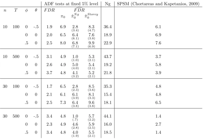
(16) N (0; 1) : Finally, the idiosyncratic component uit is ARMA(1,1):. (1. L) uit = (1 + L) "it. and "it s i:i:d:N (0; 1) : We consider three values for each of. and ; -.5,. 0, and .5 but do not consider cases where the roots cancel each other out. This means that we have a total of 7 pairs of. and : To preserve space,. and as the results change in an obvious way with for. 0. 0,. we report results only. = :5: We also report results only for three pairs of. uit is i.i.d. ( =. and. : when. = 0), when it has a negative MA root ( = 0; =. and when it has a positive AR root ( = :5;. :5);. = 0). We have also looked. at the case where the units are cross-sectionally independent (which we can interpret as. i. = 0 for all i): Results for other ( ; ) pairs and for independent. cross-sections are very similar to those reported here. All other results are available upon request. We consider the n null hypotheses that each series has a unit root. We use an ADF test for this purpose. We choose the degree of augmentation in the regression with the MAIC or Ng and Perron (2001) with a maximum of 4 lags. We consider two choices of n and T; n = 10; 30 and T = 100; 500: We do not consider larger choices of n because of the heavy computational burden imposed by the bootstrap procedure of Romano et al. (2008) : We run each experiment 1000 times. In Table 1, we report the average F DP over the replications (which ap-. 14.

(17) proaches F DR as the number of replications increases) for a …xed test size of 5% and three (conservative) estimates that di¤er according to the choice of ^ 0 : The …rst one uses the true. 0. (and is therefore infeasible), the second. uses Ng’s estimator (4), and the last one uses Storey’s estimator (3) : We report both the mean and standard deviation of the last two estimators. From this table, we …rst notice that F DR estimators can be quite conservative. Secondly, there is not much e¤ect of either n or T on the estimators. Finally, the relative performance of these estimators follows that of the estimators of. 0:. Because Ng’s estimator of. 0. is less biased but more volatile,. the estimator of F DR based on it is less biased but more variable in general. However, it behaves quite poorly in the large MA cases because the estimator inherits the large size distortions of univariate unit root tests see Schwert, 1989). The negative MA root makes the observed series look like a stationary series, thus biasing the estimator of. 0. downward.. In the last two columns of table 1, we compare with two other methods of classifying series into I (0) and I (1) units. The …rst method was proposed by Ng (2008) : After having estimated the fraction of nonstationary series, one can order the series according to the estimated largest autoregressive root and treat the ^ 0 n series with the highest roots as non stationary and the rest as stationary. The second method we consider is the Sequential Panel Selection Method (SPSM) of Chortareas and Kapetanios (2009) which is based on a series of unit root tests on panels of decreasing dimensions. Because our DGP includes cross-sectional dependence, we use the CIP S test of Pesaran (2007) 15.

(18) as the panel unit root test in the procedure (Chortareas and Kapetanios used the Im et al. (2003) test which assumes cross-sectional independence). In the last two columns of table 1, we report the F DR of these two methods. Note that these quantities cannot be estimated in practice and that one cannot use some estimated F DR as the basis for comparing classi…cation methods. Since neither method is geared towards control of the F DR; it is not surprising that both methods have a higher F DR than the method based on individual tests. Secondly, one can note that Ng’s method has much higher F DR than other methods. Finally, the SPSM does well in terms of F DR and is competitive with a sequence of individual tests. In table 2, we change our approach and report results when we try to control the F DR at 5%. We consider three methods described above. The …rst one is the original Benjamini and Hochberg (BH) method that compares the p-values to an increasing sequence of critical values. This method implicitly assumes that all null hypotheses are correct (. 0. = 1). The second method. is the modi…ed BH method (denoted BH ) which uses the Ng estimator of 0. when calculating the increasing critical values. Finally, we report the. bootstrap-based method of Romano et al. (2008) implemented as described above. If the methods controlled the F DR perfectly, we would expect 5% in all cells in the table. Numbers below 5% indicate that the method controls the F DR since the proportion of false rejections is less than the desired level of 5%. However, it lacks power since we could have rejected other null hypotheses without violating the F DR constraint. 16.

(19) The …rst thing to note from the table is that the original BH method is very conservative. Despite a desired level of 5%, we reject much less often than that. This is due to the fact that BH assumes that. 0. = 1 when. constructing the critical values. On the other hand, using the Ng estimator of. 0. alleviates these problems as expected. However, in the cases with large. MA components, the F DR is not controlled at all and the method performs quite poorly. Finally, the bootstrap method of Romano et al. performs really well in obtaining an F DR of approximately 5% even in the large MA cases were the modi…ed BH procedure performs poorly.. 6. Conclusion. In this paper, we demonstrate how to use the F DR in evaluating I(1)=I(0) classi…cations based on individual unit root tests. In the literature, most of the analysis of the F DR have been done under independence. Yet, in many interesting applications, cross-sectional data are not independent, and sometimes this dependence is quite strong. As developed here, the methods used to control or dependence require the use of the joint distribution of the test statistics. To obtain an estimate of this distribution, we rely on the bootstrap, and this method is subject to the curse of dimensionality. Application to panels with a large number of cross-sections would probably require the use of a parametric model of dependence such as a factor or spatial model.. 17.

(20) References [1] Andrews, D. (1991): Heteroskedasticity and Autocorrelation Consistent Covariance Matrix Estimation, Econometrica, 59, 817–858. [2] Bajgrowicz, P. and O. Scaillet (2009): Technical Trading Revisited: False Discoveries, Persistence Tests, and Transaction Costs, Mimeo. [3] Barras, L., O. Scaillet, and R. Wermers (2010): False Discoveries in Mutual Fund Performance: Measuring Luck in Estimated Alphas, Journal of Finance, LXV, 179-216. [4] Benjamini, Y. and Hochberg, Y. (1995):. Controlling the false discovery rate: a practical and powerful approach to multiple testing, Journal of the Royal Statistical Society, Series B, 57, 289-300. [5] Benjamini, Y. and Yekutieli, (2001): The Control of the False Discovery Rate in Multiple Testing under Dependency, The Annals of Statistics, 29, 1165-1188. [6] Breitung, J. and M. H, Pesaran (2008): Unit Roots and Cointegration in Panels, in Matyas, L. and P. Sevestre (eds.), The Econometrics of Panel Data (Third Edition), Kluwer Academic Publishers, 279-322. [7] Chortareas, G., and G. Kapetanios (2008): Getting PPP Right: Identifying Mean-reverting Real Exchange Rates in Panels, Journal of Banking and Finance, 33, 390-404. [8] Deckers, T. and C. Hanck (2009): Multiple Testing Techniques in Growth Econometrics. Mimeo. [9] Gonçalves, S. (2010): The Moving Blocks Bootstrap for Panel Linear Regression Models with Individual Fixed E¤ects, Econometric Theory, forthcoming. [10] Hanck, C. (2009): For Which Countries did PPP hold? A Multiple Testing Approach, Empirical Economics 37, 93-103. [11] Holm, S. (1979): A Simple Sequentially Rejective Multiple Test Procedure, Scandianavian Journal of Statistics, 6, 65-70.. 18.

(21) [12] Hounkannounon, B. (2009): Bootstrap for Panel Regression Models with Random E¤ects, Mimeo, Université de Montréal. [13] Im, K.S., M.H. Pesaran, and Y. Shin (2003): Testing for Unit Roots in Heterogeneous Panels, Journal of Econometrics, 115, 53-74. [14] Lehmann, E.L. and J.P. Romano (2005): Testing Statistical Hypotheses, 3rd Ed. Springer. [15] Moon, H.R. and B. Perron (2004): Testing for a Unit Root in Panels with Dynamic Factors, Journal of Econometrics; 122, 81-126. [16] Ng, S. (2008): A Simple Test for Non-Stationarity in Mixed Panels, Journal of Business and Economic Statistics , 26, 113-127 [17] Ng, S. and P. Perron (2001): Lag Length Selection and the Construction of Unit Root Tests with Good Size and Power, Econometrica, 69, 15191554. [18] Palm, F.C., S. Smeekes, and J.-P. Urbain (2008): Cross-Sectional Dependence Robust Block Bootstrap Panel Unit Root Tests, METEOR Research Memorandum 0RM/08/048, Mimeo. [19] Pesaran, M. H. (2007): A Simple Panel Unit Root Test in the Presence of Cross Section Dependence, Journal of Applied Econometrics, 22, 265312. [20] Romano, J. P., A.M. Shaikh, and M. Wolf (2008): Control of the False Discovery Rate under Dependence using the Bootstrap and Subsampling, Test, 17, 417-442. [21] Schwert, G. W. (1989): Tests for Unit Roots: A Monte Carlo Investigation, Journal of Business and Economic Statistics, 7, 147-159. [22] Storey, J.D. (2003): "The Positive False Discovery Rate: A Bayesian Interpretation and the q-value", Annals of Statistics, 31, 2013-2035 [23] Storey, J. D., J. Taylor, and D. Siegmund (2004), “Strong control, conservative point estimation and simultaneous conservative consistency of false discovery rates: a uni…ed approach, Journal of the Royal Statistical Society B, 66, 187-205.. 19.

(22) Table 1. F DR and estimates of F DR (%) for di¤erent classi…cation schemes. n. T. 10. 100. 10. 30. 30. 500. 100. 500. ADF tests at …xed 5% level F DR Fd DR Ng ^ ^ Storey 0 0 0 0. -.5. 1.9. 6.9. 0. 0. 2.0. 6.5. .5. 0. 2.5. 8.0. 0. -.5. 3.1. 4.9. 0. 0. 2.6. 4.9. .5. 0. 3.7. 4.8. 0. -.5. 1.7. 6.5. 0. 0. 2.1. 6.1. .5. 0. 2.5. 7.3. 0. -.5. 3.4. 4.8. 0. 0. 2.3. 4.9. .5. 0. 3.4. 4.8. 2:8. (3:4). Ng. SPSM (Chortareas and Kapetanios, 2009). 8:3. 36.4. 6.1. 7:6. 18.9. 6.9. 9:9. 22.9. 7.6. 5:3. 43.7. 3.7. 5:4. 19.2. 5.8. 5:2. 21.8. 3.9. 8:5. 35.3. 4.8. 8:1. 15.4. 4.8. 9:6. 18.1. 6.5. 5:7. 44.1. 1.4. 5:9. 16.0. 2.7. 5:5. 18.5. 1.4. (4:7). 6:4. (6:1). (3:8). 6:8. (7:1). (6:9). 1:0. (1:0). (2:1). 5:0. (4:0). (2:1). 4:1. (3:2). (2:1). 2:8. (2:3). (3:6). 6:1. (3:9). (3:3). 6:4. (3:8). (3:8). 1:0 (:7). (2:2). 4:6. (2:8). (2:5). 4:0. (1:9). (2:1). Note: The …rst column reports the proportion of false rejections. The next three columns report estimates of the false discovery rate using 0 ; Ng’s estimator of 0 , and Storey’s estimator of 0 with data-dependent choice of : Finally, the last two columns report the false discovery rate associated with di¤erent classi…cation schemes, one based on Ng’s ordering autoregressive roots and Chortareas amd Kapetanios’s scheme based on a sequence of panel unit root tests.. Table 2. F DR control (%) n. T. BH. BH. RSW. 10. 100. 0 0 .5. -.5 0 0. 1.0 .9 .6. 14.3 6.5 8.5. 4.0 3.2 4.8. 10. 500. 0 0 .5. -.5 0 0. 1.8 1.5 2.1. 21.4 9.5 12.1. 6.8 5.6 6.2. 30. 100. 0 0 .5. -.5 0 0. .6 .9 .8. 16.2 3.5 4.4. 3.8 3.5 4.0. 30. 500. 0 0 .5. -.5 0 0. 1.8 1.1 1.9. 34.0 5.0 7.4. 7.0 5.2 8.4. Note: The table reports the proportion of false rejections using the Benjamini-Hochberg method and the bootstrap method of Romano et al. (2008) with a desired FDR level of 5%..

(23)