Shape analysis for assessment of progression in spinal
deformities
by
Edgar Eduardo GARCÍA CANO CASTILLO
MANUSCRIPT-BASED THESIS PRESENTED TO ÉCOLE DE
TECHNOLOGIE SUPÉRIEURE IN PARTIAL FULFILLMENT OF THE
REQUIREMENTS FOR THE DEGREE OF DOCTOR OF PHILOSOPHY
Ph.D.
MONTREAL, JANUARY 24, 2019
ÉCOLE DE TECHNOLOGIE SUPÉRIEURE UNIVERSITÉ DU QUÉBEC
This Creative Commons license allows readers to download this work and share it with others as long as the author is credited. The content of this work can’t be modified in any way or used commercially.
BOARD OF EXAMINERS
THIS THESIS HAS BEEN EVALUATED BY THE FOLLOWING BOARD OF EXAMINERS
Mr. Luc Duong, Thesis Supervisor
Department of Software and IT Engineering, École de technologie supérieure
Mr. Fernando Arámbula Cosío, Thesis Co-supervisor
Instituto de Investigaciones en Matemáticas Aplicadas y en Sistemas, National University of Mexico
Mr. Mohamed Cheriet, President of the Board of Examiners
Automated Production Engineering Department, École de technologie supérieure
Mrs. Sylvie Ratté, Member of the jury
Department of Software and IT Engineering, École de technologie supérieure
Mr. Jonathan Boisvert, External Evaluator National Research Council Canada
THIS THESIS WAS PRENSENTED AND DEFENDED
IN THE PRESENCE OF A BOARD OF EXAMINERS AND PUBLIC ON JANUARY 17, 2019
ACKNOWLEDGMENT
First, I would like to thank my supervisor, Prof. Luc Duong, who gave me the opportunity to work on this fascinating research topic. Thank you for your guidance, advice and support outside and inside the research world. Thank you for sharing your expertise and the “step by
step” philosophy.
I want to thank my co-supervisor Prof. Fernando Arámbula Cosío for his counsel and assistance during this adventure. I will always be thankful for the trust you put in me since my Master’s degree in Mexico. That trust changed my life.
I thank the board of examiners, Sylvie Ratté, Mohamed Cheriet and Jonathan Boisvert, for accepting to review my thesis and providing me with valuable insights about my research project.
I thank our collaborators in the Laboratoire Informatique de la Scoliose 3D (LIS3D) at Sainte-Justine Hospital, Christian Bellefleur, Marjolaine Roy-Beaudry, Julie Joncas, Dr. Stefan Parent and Dr. Hubert Labelle who contribute with priceless knowledge and efforts to improve the health of many patients.
I also express my gratitude to Fabian Torres and Zian Fanti who were always available to share their expertise about ultrasound. I would like to thank the technical staff at ETS: Patrice Dion, Samuel Docquier, and Olivier Rufiange, who were always available to help me with technical issues/problems during my research.
I also want to express my gratitude to all LINCS and LIVE members. Thank you for your invaluable help and support, especially in the last sprint.
To my mother, Hortencia and my brother, Eric, thank you a lot for all you blind support and to be there unconditionally, in every up and down of this roller coaster called life. For supporting me no matter what in every step, in each adventure that has led me to this moment.
So many centuries, so many worlds, so much space, and we coincided. Thank you, Laura, for having stepped on the gas pedal, for your company, friendship and support, but specially, for being my partner in crime.
Lorena and Alejandro, thank you for friendship, for all the gatherings, but particularly, for your support during difficult moments.
A very special thanks to my friends Ricardo, Marc, Foti, the MFO team, the volleyball team, and the broadcasters of Frikipodcast and Palomazo podcast, whom directly or indirectly were companions in this trip.
Finally, this research was conducted thanks to the financial support of the Consejo Nacional
de Ciencia y Tecnología, Mexico (CONACYT; 323619) and the Fonds de recherche du
Québec – Nature et technologies (FRQNT; 194703), and the Ministère des Relations internationales et de la Francophonie.
Analyse de formes pour le suivi de la progression en Scoliose Idiopathique Adolescente
Edgar Eduardo GARCIA CANO CASTILLO
RÉSUMÉ
La scoliose idiopathique adolescente (SIA) est une déformation tridimensionnelle de la colonne vertébrale. Elle se manifeste généralement par une déviation latérale du rachis dans le plan postéro-antérieur. La SIA peut se manifester dès le début de la puberté, touchant entre 1 et 4 % de la population adolescente âgée de 10 à 18 ans, les jeunes femmes étant les plus touchées. Certains cas graves (0,1% de la population avec AIS) nécessiteront un traitement chirurgical visant à corriger la courbure scoliotique.
A ce jour, le diagnostic de la SIA repose sur l’analyse des radiographies postéro-antérieures et latérale et la sévérité de la courbure est déterminée par la méthode de l'angle de Cobb. Cet angle est calculé en traçant deux lignes parallèles. Une ligne parallèle à la plaque d'extrémité supérieure de la vertèbre la plus inclinée en haut de la courbe et une ligne parallèle à la plaque d'extrémité inférieure de la vertèbre la plus inclinée en bas de la même courbe. Les patients qui présentent un angle de Cobb supérieur à 10° sont diagnostiqués avec la SIA.
La mesure étalon pour classer les déformations des courbures scoliotiques est la méthode de Lenke. Cette classification est largement acceptée dans la communauté clinique divise les patients atteints de scoliose en six types et fournit des recommandations de traitement selon le type. Cette méthode se limite à l'analyse de la colonne vertébrale dans l'espace 2x2D, puisqu'elle repose sur l'observation de radiographies et de mesures de l'angle de Cobb.
D'un côté, lorsque les cliniciens traitent des patients atteints de SIA, l'une des principales préoccupations est de déterminer si la déformation évoluera avec le temps. Le fait de connaître à l'avance l'évolution de la forme de la colonne vertébrale aiderait à orienter les stratégies de traitement. D’un autre côté, les patients à plus haut risque d'évolution doivent être suivis plus fréquemment, ce qui entraîne une exposition accrue aux rayons-X. Par conséquent, il est nécessaire de mettre au point une autre technologie sans radiations pour réduire l'utilisation des radiographies et atténuer les dangers d'autres problèmes de santé découlant des modalités actuelles d'imagerie.
Cette thèse présente une méthode pour l’évaluation de la forme de la colonne vertébrale de patients atteints de SIA. Elle comprend trois contributions : 1) une nouvelle approche pour calculer les descripteurs 3D de la colonne vertébrale, et une méthode de classification pour catégoriser les déformations de la colonne vertébrale selon la classification de Lenke, 2) une méthode pour analyser la progression dans le temps de la colonne vertébrale et 3) un protocole d’acquisition pour générer un modèle 3D de la colonne à partir d'une reconstruction de volume produite par des images échographiques.
Dans notre première contribution, nous avons présenté deux techniques de mesure pour caractériser la forme de la colonne vertébrale dans l'espace 3D. De plus, une méthode d'ensemble dynamique a été présentée comme une alternative automatisée pour classer les déformations de la colonne vertébrale. Ces techniques de mesure pour calculer les descripteurs 3D sont faciles à appliquer dans les installations cliniques. En outre, la méthode de classification contribue en aidant les cliniciens à identifier les descripteurs propres à chaque patient, ce qui pourrait aider à améliorer la catégorisation des déformations à la limite et, par conséquent, les traitements.
Afin d'observer la progression du rachis dans le temps, nous avons conçu une méthode pour simuler la variation de la forme depuis la première visite jusqu'à 18 mois. Cette simulation montre les changements de forme tous les trois mois. Notre méthode est entraînée avec des modes de variation, calculés à l'aide d'une analyse par composantes indépendantes à partir de reconstructions de modèles 3D de la colonne vertébrale de patients atteints de SIA. Chacun des modes de variation peut être visualisé pour interprétation. Cette contribution pourrait aider les cliniciens à identifier les déformations de la colonne vertébrale qui pourraient progresser. Le traitement peut donc être adapté en fonction des besoins de chaque patient.
Finalement, notre troisième contribution porte sur la nécessité d'une modalité d'imagerie sans radiations pour l'évaluation et la surveillance des patients atteints de SIA. Nous avons proposé un protocole pour modéliser la colonne vertébrale d'un sujet en marquant la position des apophyses sur une reconstruction volumique. Cette reconstruction a été calculée à partir d’images échographique acquises sur la surface externe du patient. Notre protocole fournit un guide étape par étape pour établir un dispositif d'acquisition d'images, ainsi que des recommandations à prendre en compte en fonction de la composition corporelle des sujets à reconstruire. Nous croyons que ce protocole pourrait contribuer à réduire l'utilisation des radiographies lors de l'évaluation et du suivi des patients atteints de SIA.
Mots clés : Scoliose idiopathique adolescente ; classification de la colonne vertébrale ;
sélection dynamique d'ensemble ; descripteurs de la colonne vertébrale ; prédiction de la progression du rachis ; analyse par composantes indépendantes ; apprentissage machine ; échographie 3D à main levée ; échographie ; reconstruction de la colonne.
Shape analysis for assessment of progression in spinal deformities
Edgar Eduardo GARCIA CANO CASTILLO
ABSTRACT
Adolescent idiopathic scoliosis (AIS) is a three-dimensional structural spinal deformation. It is the most common type of scoliosis. It can be visually detected as a lateral curvature in the postero-anterior plane. This condition starts in early puberty, affecting between 1-4% of the adolescent population between 10-18 years old, affecting in majority female. In severe cases ( 0.1% of population with AIS) the patient will require a surgical treatment. To date, the diagnosis of AIS relies on the quantification of the major curvature observed on posteroanterior and sagittal radiographs.
Radiographs in standing position are the common imaging modality used in clinical settings to diagnose AIS. The assessment of the deformation is carried out using the Cobb angle method. This angle is calculated in the postero-anterior plane, and it is formed between a line drawn parallel to the superior endplate of the upper vertebra included in the scoliotic curve and a line drawn parallel to the inferior endplate of the lower vertebra of the same curve. Patients that present a Cobb angle of more than 10°, are diagnosed with AIS.
The gold standard to classify curve deformations is the Lenke classification method. This paradigm is widely accepted in the clinical community. It divides spines with scoliosis into six types and provides treatment recommendations depending on the type. This method is limited to the analysis of the spine in the 2D space, since it relies on the observation of radiographs and Cobb angle measurements.
On the one hand, when clinicians are treating patients with AIS, one of the main concerns is to determine whether the deformation will progress through time. Knowing beforehand of how the shape of the spine is going to evolve would aid to guide treatments strategies. On the other hand, however, patients at higher risks of progression require to be monitored more frequently, which results in constant exposure to radiation. Therefore, there is a need for an alternative radiation-free technology to reduce the use of radiographs and alleviate the perils of other health issues derived from current imaging modalities.
This thesis presents a framework designed to characterize and model the variation of the shape of the spine throughout AIS. This framework includes three contributions: 1) two measurement techniques for computing 3D descriptors of the spine, and a classification method to categorize spine deformations, 2) a method to simulate the variation of the shape of the spine through time, and 3) a protocol to generate a 3D model of the spine from a volume reconstruction produced from ultrasound images.
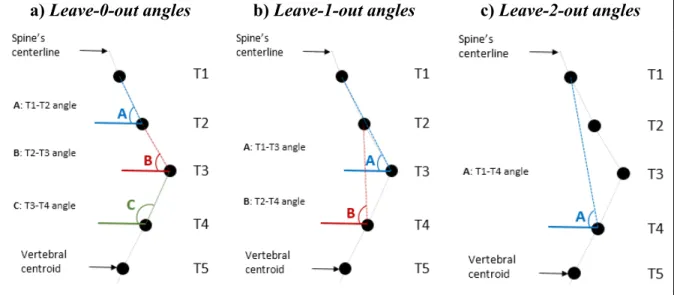
In our first contribution, we introduced two measurement techniques to characterize the shape of the spine in the 3D space, leave-n-out, and fan leave-n-out angles. In addition, a dynamic ensemble method was presented as an automated alternative to classify spinal deformations. Our measurement techniques were designed for computing the 3D descriptors and to be easy to use in a clinical setting. Also, the classification method contributes by assisting clinicians to identify patient-specific descriptors, which could help improving the classification in borderline curve deformations and, hence, suggests the proper management strategies.
In order to observe how the shape of the spine progresses through time, in our second contribution, we designed a method to visualize the shape’s variation from the first visit up to 18 months, for every three months. Our method is trained with modes of variation, computed using independent component analysis from 3D model reconstructions of the spine of patients with AIS. Each of the modes of variation can be visualized for interpretation. This contribution could aid clinicians to identify which spine progression pattern might be prone to progression. Finally, our third contribution addresses the necessity of a radiation-free image modality for assessing and monitoring patients with AIS. We proposed a protocol to model a spine by identifying the spinous processes on a volume reconstruction. This reconstruction was computed from ultrasound images acquired from the external geometry of the subject. Our acquisition protocol documents a setup for image acquisition, as well as some recommendations to take into account depending on the body composition of the subjects to be scanned. We believe that this protocol could contribute to reduce the use of radiographs during the assessment and monitoring of patients with AIS.
Keywords: Adolescent idiopathic scoliosis; spine classification; dynamic ensemble selection;
descriptors of the spine; prediction of spinal curve progression; independent component analysis; machine learning; freehand 3D ultrasound; tracked ultrasound; spine reconstruction.
TABLE OF CONTENTS
Page
INTRODUCTION ...1
0.1 Problem statement and motivation ...2
0.2 Research objectives and contributions ...3
0.3 Outline ...5
CHAPTER 1 LITERATURE REVIEW ...3
1.1 Clinical context ...3
1.1.1 Anatomy of the spine ... 3
1.1.2 Sections of the spine ... 3
1.1.3 Curves of the spine ... 5
1.1.4 Adolescent Idiopathic Scoliosis: characterization and classification ... 6
1.2 State-of-the-art on computer-based characterization and classification methods in Adolescent Idiopathic Scoliosis using 3D descriptors ...9
1.3 State-of-the-art on computer-generated models for progression of the curve of the spine through time ...14
1.4 State-of-the-art on radiation-free imaging systems to reduce the use of X-rays. ...16
1.5 Summary ...24
CHAPTER 2 DYNAMIC ENSEMBLE SELECTION OF LEARNER-DESCRIPTOR CLASSIFIERS TO ASSESS CURVE TYPES IN ADOLESCENT IDIOPATHIC SCOLIOSIS ...27
2.1 Abstract ...27
2.2 Introduction ...28
2.3 Methods ...30
2.3.1 Dataset ... 30
2.3.2 Descriptors of the spine ... 31
2.3.3 Ensemble learning ... 33
2.4 Experimental setup ...37
2.4.1 Base learning algorithm ... 37
2.4.2 Feature selection ... 38 2.4.3 Classification ... 38 2.5 Results ...39 2.5.1 Feature selection ... 39 2.5.2 Classification ... 40 2.6 Discussion ...42 2.7 Conclusions ...44
CHAPTER 3 PREDICTION OF SPINAL CURVE PROGRESSION IN ADOLESCENT IDIOPATHIC SCOLIOSIS USING RANDOM FOREST REGRESSION ....47
3.2 Introduction ...48
3.3 Methods ...51
3.3.1 3D spine models ... 51
3.3.2 Descriptors of the spine ... 54
3.3.3 Spinal curve shape prediction ... 55
3.4 Results ...57
3.4.1 Descriptors of the spine ... 57
3.4.2 Shape prediction ... 60
3.5 Discussion ...64
3.6 Conclusion ...71
CHAPTER 4 A FREEHAND ULTRASOUND FRAMEWORK FOR SPINE ASSESSMENT IN 3D: A PRELIMINARY STUDY ...73
4.1 Abstract ...73
4.2 Introduction ...74
4.3 Materials and Methods ...77
4.3.1 Freehand 3D ultrasound system ... 77
4.3.2 Study subjects ... 77
4.3.3 Acquisition protocol ... 78
4.3.4 3D reconstruction of the spine ... 81
4.3.5 Anatomical landmark identification ... 82
4.3.6 Posture quantification ... 83
4.4 Results ...84
4.4.1 Volume reconstructions ... 85
4.5 Discussion ...89
4.6 Conclusions ...98
CHAPTER 5 DISCUSSION AND CONCLUSION ...101
LIST OF TABLES
Page
Table 1.1 Characteristics of included studies ...10
Table 1.2 Methodology of included studies ...12
Table 1.3 Hardware used for US image acquisition ...23
Table 2.1 Description of the classes in the dataset ...30
Table 2.2 Distribution of the dataset ...30
Table 2.3 Descriptors generated from a dataset of 3D spine models ...31
Table 2.4 Example of the analysis of one test sample using the 3 highest ranked LDCs per class. a) displays the rank of 6 LDCs per class, computed during the training phase. b) shows the classifiers that were employed to perform a prediction on the nn, which belongs to class 1 (LDC_1, LDC_2 and LDC_3). Then, the DES ensembles LDC_1 and LDC_3 to perform the prediction of the test sample, which were the ones that predicted correctly the nn. The crossed LDCs were discarded for the prediction. ...37
Table 2.5 Feature selection based on importance scores ...39
Table 2.6 Best descriptors employed in the test phase of the DES (steps 4.c.i to iv in Algorithm 2.1) ...41
Table 2.7 Accuracy of the classification ...41
Table 2.8 Log loss of the classification ...41
Table 2.9 Descriptive statistics of accuracy and log loss ...41
Table 2.10 Results of Friedman's test, considering 2 degrees of freedom, significance level α = 0.05, and critical value pα = 5.99 ...43
Table 2.11 Results of Wilcoxon Sign-Rank Test, on the results using the log loss metric, with a Bonferroni correction and significance level p < 0.017 ...44
Table 3.1 Variation of independent components, obtained from the 3D models of the spines with respect to the mean shape. ...58 Table 3.2 Average scores by layer of the prediction models using the descriptors obtained
from ICA and SDAE after 10-fold cross-validation. Four root-mean-squared errors (RMSE) were calculated. 3D indicates the error in the three-dimensional
space. PAP, SP and AP show the RMSE in the posteroanterior, sagittal and
apical planes, respectively. Each row indicates a layer in the scheme. ...61
Table 3.3 Prediction of the shape of the spines (centerline) of two patients in the posteroanterior (PAP), sagittal (SP) and apical (AP) planes. The first and second rows belong to the schemes using descriptors from ICA, while the third and fourth rows correspond to the descriptors from SDAE. Shapes in rows 1 and 3 were obtained with scheme a, and shapes in rows 2 and 4 were obtained with scheme b. The grey shape represents the original shape, while the black shape depicts the predicted one. ...62
Table 3.4 Averages and standard deviations of the differences in Cobb angles, in the proximal thoracic (PT), main thoracic (MT) and thoraco-lumbar lumbar (TL/L) sections, between the predicted and the original shapes of the spine after the 10-fold cross-validation. Each row indicates a layer in the scheme. ...64
Table 3.5 Significance of correlation of ICs at first visit with progression ...69
Table 4.1 Anthropometric characteristics of the subjects involved in this study ...84
Table 4.2 Statistics per one sweep in different setups. As part of the acquisition, time (seconds), number of frames and disk space (megabytes) used are presented. Also, disk space (megabytes) after selection the region of interest is displayed, together the reconstruction time and disk space for each computed reconstruction. ...85
Table 4.3 Differences of the first three 3D point-based models of the spine with respect to the fourth in experiment 1 ...87
Table 4.4 Differences between two models obtained from an unconstrained setup ...87
Table 4.5 Differences between the fast and the fourth model of experiment 1 ...88
Table 4.6 Differences between the slow and the fourth model of experiment 1 ...88
LIST OF FIGURES
Page Figure 1.1 The five sections of the spine, and numbering of the vertebrae. Adapted from:
Henry Gray (1918) Anatomy of the Human. Altered by User: Uwe Gille, public domain. ...4 Figure 1.2 Spines and its abnormal curvatures. ...5 Figure 1.3 Global coordinate system. Adapted from: Wikimedia Commons used under
Creative Common created by CFCF, June 2014. ...6 Figure 1.4 Cobb angle measurements for 2 patients using a different geometrical
construction. Photo courtesy of Prof. Frank Gaillard, Radiopaedia.org, adapted under Creative Common license. ...7 Figure 1.5 Two different braces to treat scoliosis. Chêneau brace on the left and Chêneau
light on the right. Adapted from Wikimedia Commons used under Creative Common license. Created by Scolidoc (Weiss et al. Scoliosis 2007 2:2
doi:10.1186/1748-7161-2-2). ...8 Figure 1.6 On the left, a patient before surgery. On the right, the patient after surgery.
Photo courtesy of LIS3D, Sainte-Justine Hospital. ...9 Figure 2.1 Leave-n-out angles calculation with respect to the horizontal axis, with n=0 to
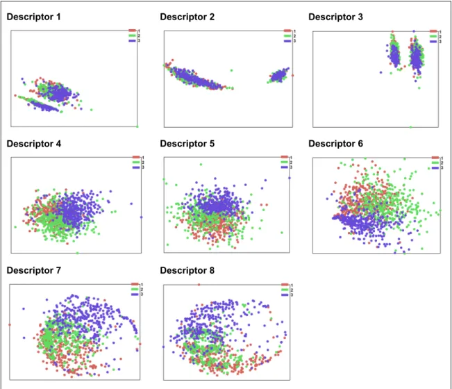
n=2 ...32 Figure 2.2 Fan Leave-n-out angles calculation for n=0, and n=1 ...33 Figure 2.3 Visualization of the best features of each of the eight descriptors employing
multidimensional scaling ...40 Figure 3.1 Three cases of interpolated 3D models of the spine. The black triangles
correspond to models of actual visits. If they were within 30 days of the cut-off time for an interval, they were preserved in the dataset as the models for that interval. Black squares represent interpolated models generated based on the nearest actual models. ...53 Figure 3.2 Schemes for shape prediction. Scheme a uses only the immediate output of the
past visit as input for the next layer. Scheme b takes all previous outputs as input for the next layer. ...56 Figure 3.3 Architecture of the stacked denoising autoencoders. The layer in the center (9) is
Figure 4.1 Image acquisition setup: the electro-magnetic measurement system, US scanner,
and workstation. ...79
Figure 4.2 One acquisition has 3 sweeps. The white boxes indicate the positions of the probe in each sweep. ...79
Figure 4.3 Identification of vertebrae by the operator ...80
Figure 4.4 Localization of the intervertebral space between the L4 and L5 vertebrae ...80
Figure 4.5 Fix reference sensor on the subject, 3 inches to the left from the centerline ...80
Figure 4.6 a) original raw image with dark margins and configuration from the US. b) cropped image showing the region of interest. ...82
Figure 4.7 Identification of spinous processes ...83
Figure 4.8 Calculation of the angle formed by two adjoint vertebrae (black dots) with respect to the horizontal axis in the lumbar section, from two planes ...84
Figure 4.9 Volume reconstruction of the spine of three subjects ...86
Figure 4.10 Subjects with different body composition. Subject S-2 has the leanest mass. Subject S-3 is not muscular, but slim build. Subjects 6 and 8 have healthy body compositions. ...89
Figure 4.11 Problematic region on thoracolumbar/lumbar section of the spine due to the stiffness of the muscles in subjects S-2 and S-7. ...91
Figure 4.12 Motion in reconstructions from constrained (left) and unconstrained (right) setups ...95
Figure 4.13 On the left, a sagittal view of four thoracic vertebrae. On the right a frontal view of the same vertebrae. Red dots indicate the spinous processes, and orange dots indicate the laminae ...97
LIST OF ABREVIATIONS
AIS Adolescent idiopathic scoliosis ATR Angle of trunk rotation
AVL Apical vertebra level AVR Apical vertebrae rotation BFP Best fit plane
C° Cobb angle
COL Center of lamina
CPM Center of pedicle method
CT Computed Tomography
FBT Forwarded bending test
FH3DUS Freehand 3D ultrasound system GT Geometric torsion
ICC Intra correlation coefficient MRI Magnetic Resonance Imaging
MT Main thoracic
PA Posteroanterior plane PMC Plane of maximum curvature PT Proximal thoracic
SAP Superior articular process SP Spinous process
SRS Scoliosis research society SS Sanders Stage TLL Thoracolumbar/lumbar TP Transverse process US Ultrasound 2D Two dimensions 3D Three dimensions
INTRODUCTION
Adolescent Idiopathic Scoliosis (AIS) is a 3D deformation of the spine, mainly visible as a lateral curvature in the form of an elongated “S” or “C” shape from the posteroanterior plane. AIS is the most common type of scoliosis, and it is highly prevalent in adolescent between 10 and 18 years of age, or until skeletal maturity. Between 1% to 4% of the adolescent population− mainly girls−is affected by AIS. AIS starts in early puberty, a time when children are growing rapidly, and although not all the curves will be progressive, 1 over 1000 will require a surgical treatment.
The “idiopathic” part of AIS means that the cause is not known. However, genetic studies indicate that there exists an increased risk of developing AIS when there are first degree relatives with this condition. In addition, AIS can be related to other factors such as environmental, central nervous system abnormalities, skeletal and muscle growth, hormonal and metabolic, or other factors not yet identified.
AIS is usually diagnosed by a physical examination or postural screening exam at school. Common signs of AIS are asymmetry in shoulder height or shift of the trunk, where the hips look uneven, which cause that one leg appears to be longer than the other. In addition, a back hump can be visualized when the patient is bending forward.
Clinical assessment and classification of IAS rely on 2D radiographic observations of the spine in the posteroanterior and sagittal planes. These radiographs are taken in a standing position having a full view of the shape of the spine. A sense of abstraction is needed by clinicians who evaluate these projections to figure not only how the spine looks in the 3D space, but also how the curvature will progress.
Advances in technology are changing the current 2D description of AIS towards a 3D characterization. These 3D descriptors could be important to improve the understanding of AIS, as well as to improve assessment, prediction of progression and treatment.
0.1 Problem statement and motivation
The goal of studying scoliosis is to understand the medical condition, and to select the optimal treatment or surgical strategy for each patient. Since the spine is a 3D structure, experts who evaluate 2D images of the spine need experience, abstraction and visualization skills in order to avoid misinterpretation. Likewise, the evaluation is not deterministic and can change from expert to expert.
The current gold standard for the assessment of the magnitude of the curve is a 2D measurement used to evaluate a 3D structure. Nevertheless, two patients sharing the same profile in 2D will not necessarily share the same morphology in the 3D space. Hence, the treatments should be adapted specifically to the 3D shape of the spine (Labelle et al., 2011). Recent advances in technology allow to generate new techniques to characterize the spine in the 3D space. However, these descriptors are difficult to interpret and to measure in a clinical setting where only 2D radiographs are available.
Classification methods emerge to present a way to ease the visualization of common patterns in a dataset. In the case of spine deformities, the Lenke classification method helps to group similar curves. Nevertheless, although this system is widely used in clinical practice, it does not provide a full understanding of the deformation in the 3D space, since it depends on the analysis of 2D radiographs. The importance of a 3D classification system resides in improving the description and comprehension of AIS, in a way that can be reproduced with reliable outcomes.
Prediction of the development of the curves through time is also a relevant task. Knowing beforehand how the curve could change in the future, would help clinicians to improve treatments. Clinical indices such as chronological, skeletal, and menarcheal age, curve magnitude, and curve location have been studied (Cheng et al., 2015), however these are not robust enough to predict the deformations.
Computer-based approaches to describe, classify and predict the evolution of spine deformities would help to validate manual measurements, to decrease time for evaluating and treating patients, and to improve reproducibility.
Since patients with AIS are young, their tissues are still immature and sensitive to X-rays, which is the main imaging technology used to evaluate scoliosis. Patients with high risk of progression need to be evaluated frequently, every 4 to 6 months. Some studies (Doody et al., 2000; Hoffman, Lonstein, Morin, Visscher, & Harris III, 1989; Ronckers et al., 2010; Ronckers, Doody, Lonstein, Stovall, & Land, 2008) have shown that young women are especially sensitive to the exposure to ionizing radiation. Therefore, age, gender and recurrent exposure to radiation may increase the risk of developing breast or lung cancer (Levy, Goldberg, Mayo, Hanley, & Poitras, 1996). The development of radiation-free imaging technology to monitor spinal deformities progression would be of high interest for the management of AIS.
0.2 Research objectives and contributions
This thesis presents a framework designed to characterize and model the variation of the shape of the spine affected with AIS. This framework includes three contributions: 1) two measurement techniques for computing 3D descriptors of the spine, and a classification method to categorize spine deformations, 2) a method to simulate the variation of the shape of the spine through time, and 3) a protocol to generate a 3D model of the spine from a volume reconstruction produced from ultrasound images.
Three main contributions were proposed toward this goal:
1) Computer-based characterization and classification methods in AIS using 3D
descriptors. The classification system for spine deformations developed by Lenke, is
a descriptive and reproducible method widely used in clinical practice. However, its main disadvantage is the use of the Cobb angle to quantify the deformation of the spine,
a measurement that does not describe the spine in the 3D space. We introduced two techniques to represent the variation of the spine in 3D. Also, we proposed to use a computer-based classification algorithm called dynamic ensemble selection to categorize spine deformations. The classification method does not depend on a specific learning algorithm or set of descriptors of the spine. It identifies the best combination of them to classify curve types. This could help clinicians to evaluate the role of each descriptor in a specific spine.
2) Shape analysis using computer-generated models for progression of the curve of
the spine through time. Prediction of the progression of the spine deformation is one
of the main concerns when treating patients with AIS. Knowing how the shape of the spine is going to evolve from the first visit of the patient, would help clinicians to improve treatment strategies. In this contribution, we proposed independent components analysis to describe the modes of variation of the spine in the 3D space, together with an approach to predict the curve progression from the first visit, every three months for a time lapse of eighteen months. The results show that our approach for curve progression is a promising technique, which can help to identify the variation of the shape of the spine through time.
3) A preliminary study for a radiation-free 3D imaging system based on 2-D
ultrasound. Radiation is one of the clinician’s critical concerns in patients with AIS.
Since patients are young, there is a high risk of exposure to ionizing radiation, even with low dose systems. In this contribution, we propose the use of a freehand 3D ultrasound system to generate volume reconstructions of the spine. Ultrasound is a radiation-free technology, which could help clinicians in follow-up of patients with AIS, decreasing the need of X-rays. In this study, we were able to generate a 3D representation of the centerline of the spine, by identifying landmarks on the volume reconstruction. Our results suggest that this system can be promising for the evaluation of the shape of the spine.
0.3 Outline
This manuscript is organized as follows. In Chapter 1, we presented the clinical context of AIS, as well as a review of the relevant studies related to each of the contributions of this research. Chapter 2 introduces our techniques, leave-n-out angles and fan leave-n-out angles to describe the shape of the spine in 3D space, and the dynamic ensemble selection method to categorize deformations of the spine, this work was published in the Medical and Biological
Engineering and Computing. Chapter 3 presents our approach to predict curve progression
through time, based on 3D descriptors of the spine. This chapter was published in the
Computers in Biology and Medicine. Chapter 4 presents our efforts to reduce the use of
X-ray imaging by introducing a freehand 3D ultrasound system to generate volume reconstructions of the spine. This work was submitted to the Ultrasound in Medicine and
Biology. In Chapter 5, a summary of the main contributions of this research is presented and
discusses its limitations and future work. Finally, Appendix I shows a complete list of works resulting from this research.
CHAPTER 1 LITERATURE REVIEW
The objective of this chapter is to present a general overview of the clinical context of Adolescent Idiopathic Scoliosis, as well as the state-of-the-art methods for the evaluation of spinal deformities in 2D and in 3D. This chapter starts describing the anatomy of the spine, followed by the clinical concepts associated with the clinical study of AIS. Then, a critical review of computer-based methods involved in the study of AIS is presented. At the end, this chapter includes a summary of the approaches proposed in the literature.
1.1 Clinical context 1.1.1 Anatomy of the spine
The spine is usually composed by articulated bones called vertebrae, which help keeping an upright or stand up posture. Being the main support of the human body, it is on charge of the movements of the head and torso, and it serves as a protection for the spinal cord. The spine can flex or rotate, but the grade of movement or function depends on the different sections that compose it: cervical, thoracic, lumbar, sacral and coccyx.
1.1.2 Sections of the spine
The spine is divided in five sections (see Figure 1.1), each of them is in charge of specific functionalities:
• Cervical spine (upper back): Numbered from C1-C7, is the main support of the head. It is the section with greatest range of motion, especially because the first two vertebrae are directly connected to the skull, which allow the motion of the head.
• Thoracic spine (middle back): Numbered from T1-T12. This section is on charge of the protection of the heart and lungs by holding the rib cage.
• Lumbar spine (lower back): Numbered from L1-L5. The weight of the body is supported by this region. The vertebrae that form this part of the spine are much larger in size, compared to the previous sections.
• Sacrum: It contains five fused vertebrae. Its principal purpose is to connect the spine to the hip bones.
• Coccyx: Also known as tailbone, is comprised by four fused vertebrae. It helps to keep attached the ligaments and muscles of the pelvic floor.
Figure 1.1 The five sections of the spine, and numbering of the vertebrae. Adapted from: Henry Gray (1918) Anatomy of
1.1.3 Curves of the spine
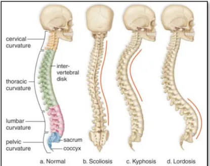
The spine naturally develops curves. When viewed from the coronal plane, it looks like a straight line. However, from the sagittal plane there are two observable curvatures in the thoracic and lumbar sections, and the aspect of the spine seems such as a soft ‘S’ shape (see Figure 1.1). These normal curves are known as kyphosis and lordosis, which are essential for the human body to keep the balance between the trunk and head over the pelvis. Both are considered normal to a certain extent.
Abnormal curvatures could be caused by congenital defects or triggered by degenerative diseases. These deformities occur when the natural curves of the spine are misaligned or surpass the acceptable limits (see Figure 1.2).
Figure 1.2 Spines and its abnormal curvatures. Adapted from StudyForce, public domain.
1.1.4 Adolescent Idiopathic Scoliosis: characterization and classification
The gold standard method to quantify the magnitude of the curves with AIS is the Cobb angle. It receives its name from Dr. Jon R. Cobb, who in 1948, first described the curvature of the spine as a measure of the magnitude of deformities. It is measured in degrees and helps physicians to determine the severity of the deformation and to decide what treatment will be necessary for the patient.
In clinical practice, the Cobb angle is measured on the posteroanterior and lateral X-rays, the most common imaging modality to observe the spine in a standing position. The radiographs are acquired based on the global coordinate system proposed by the Scoliosis Research Society (Stokes, 1994b). The x-axis is the horizontal axis that runs from the rear to the front of the patient, while the y-axis is the horizontal axis that runs from the right to the left of the patient. The z-axis is the vertical axis, which goes from the bottom of the patient upward (see Figure 1.3).
Figure 1.3 Global coordinate system. Adapted from: Wikimedia Commons used under Creative Common created by CFCF,
The Cobb angle is calculated in the postero-anterior plane, and it is formed between a line drawn parallel to the superior endplate of the upper vertebra included in the scoliotic curve and a line drawn parallel to the inferior endplate of the lower vertebra of the same curve (see Figure 1.4). If the Cobb angle is ≥ 10°, the patient is diagnosed with scoliosis.
Figure 1.4 Cobb angle measurements for 2 patients using a different geometrical construction. Photo courtesy of Prof. Frank
Gaillard, Radiopaedia.org, adapted under Creative Common license.
Classification methods arise as a way to ease the appreciation of common patterns. In AIS, a comprehensive classification system is relevant because it allows to identify all types of curve patterns, and hence to standardize the assessment and treatment. A classification method should have good to excellent inter- and intra- observer reliability in order to be reproducible in clinical setting. It would also provide clinicians with a common language to compare similar cases.
Concerning to AIS, King et al. proposed a classification method for severe thoracic curves (King, Moe, Bradford, & Winter, 1983). They classify the spines in 5 types, excluding thoracolumbar, lumbar, or double or triple major curves. However, poor inter- and intra-observer reliability and reproducibility of the method has been reported (Lenke et al., 1998). In 2001, a new classification system of AIS was developed by Lenke et al. Nowadays, the system has been widely accepted in clinical setups (Lenke et al., 2001). This categorization
divides the spine deformities in 6 types. It is based on the measurement of three components: type of curve (Lenke 1-6), a lumbar modifier, and sagittal thoracic modifier. These components are used to distinguish structural and nonstructural curves in the proximal thoracic, main thoracic, and thoracolumbar/lumbar sections. According to the classification of the spine deformation, treatment recommendations are also provided. The authors reported the reliability of the classification by the kappa values of the interobserver (0.74) and intraobserver (0.893).
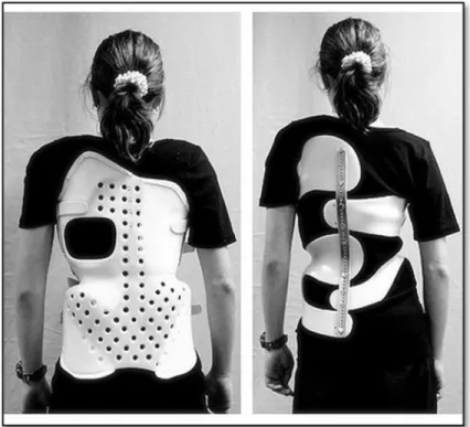
Once the patient has been diagnosed, it is feasible to provide a treatment in order to prevent the progression of the deformation, and hence, avoid surgical operation when possible. Bracing (see Figure 1.5) is prescribed for patients between 10-15 years of age, at skeletal maturity specified by the Risser grade between 0-2, and magnitude of the main curvature between 20°- 40° (Richards, Bernstein, D’Amato, & Thompson, 2005).
Figure 1.5 Two different braces to treat scoliosis. Chêneau brace on the left and Chêneau light on the right. Adapted from Wikimedia Commons used under Creative Common license. Created by Scolidoc (Weiss
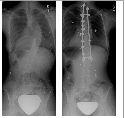
Patients at risk of curve progression during adult life, are considered for surgery (see Figure 1.6). Generally, they present curve magnitude > 50° in the thoracic section, or between 50°- 60° in the thoracolumbar section. Pain, appearance and shortness of breath are symptoms used as indicators for surgery (Asher & Burton, 2006). Patients that require surgical intervention represents 0.1% of the total with AIS (Cheng et al., 2015).
Figure 1.6 On the left, a patient before surgery. On the right, the patient after surgery. Photo courtesy of LIS3D, Sainte-Justine Hospital.
1.2 State-of-the-art on computer-based characterization and classification methods in Adolescent Idiopathic Scoliosis using 3D descriptors
A 3D classification system would help with the understanding and description of the scoliotic curves; which improve evaluation, follow-up and treatment (Labelle et al., 2011). Nowadays, technology allows to automatically collect more data, to perform measurements systematically, to generate 3D descriptors, and to create complex models to enhance the classification of the spine (Stokes, 1994a). Discovering patterns concerning the 3D space could help to introduce a
3D classification able to surpass the limitation of 2D. In addition, the Scoliosis Research Society (SRS) has accepted the need to treat AIS based on the analysis of the deformity in the 3D space (Labelle et al., 2011). Hence, the development of 3D classification method, that can be applied in everyday clinical practice, is of vital importance.
In recent studies, new classification systems based on 3D descriptors of the spine have been proposed. Negrini et al. (Negrini, Negrini, Atanasio, & Santambrogio, 2006) used an optoelectronic system (AUSCAN), generating a 3D reconstruction of the spine in real time by markers positioned on the skin of the patient. Other classification systems use 3D reconstructions of the spine obtained from standing stereographic X-rays. The reconstruction consists of 3D coordinates of particular anatomic landmarks, (Delorme et al., 2003) (see Table 1.1).
Table 1.1 Characteristics of included studies
Author Patients Classification Instrument Design
Poncet 2001 62 AIS All Lenke Stereo radiographies Prospective
Negrini 2006 122 AIS
23 hyperkyphosis 4 AIS+ hyperkyphosis
All Lenke AUSCAN Cross-sectional
Duong 2006 409 AIS All Lenke Stereo radiographies Prospective
Boisvert 2008 307 AIS Lenke 1 and 5 Stereo radiographies Cross-sectional
Sangole 2009 172 AIS right thoracic Lenke 1 Stereo radiographies Cross-sectional
Stokes 2009 110 AIS Double curves Stereo radiographies Cross-sectional
Duong 2009 68 AIS Lenke 1 Stereo radiographies Prospective
Kadoury 2012 170 AIS right thoracic Lenke 1 Stereo radiographies Cross-sectional
Kadoury 2014 65 AIS
5 healthy All Lenke Stereo radiographies Cross-sectional
Shen 2014 255 AIS Lenke 1 Stereo radiographies Cross-sectional
Thong 2015 155 AIS Lenke 1 Stereo radiographies Cross-sectional
Thong 2016 633 AIS All Lenke Stereo radiographies Cross-sectional
The descriptors of the spine can be divided by its nature in geometric or global. Geometric are measured from the 3D reconstructions of the spine, such as apical vertebra rotation (AVR), best fit plane (BFP) , direction, geometric torsion (GT), phase, plane of maximum curvature (PMC), shift (Duong, Cheriet, et al., 2009; Kadoury, Shen, & Parent, 2014; Negrini et al., 2006; Poncet, Dansereau, & Labelle, 2001; Sangole et al., 2009; Shen, Parent, & Kadoury,
2014; Stokes, Sangole, & Aubin, 2009). In a different approach, Boisvert et al. (Boisvert, Cheriet, Pennec, Labelle, & Ayache, 2008) proposed the use of rigid transformations as geometric descriptors of the spine.
On the other hand, when the descriptors are obtained by applying a method to reduce the dimensionality of the 3D reconstructions of the spine, are called global. Some descriptors have been obtained by computing a wavelet compression technique (Duong, Cheriet, & Labelle, 2006), principal component analysis (Boisvert, Cheriet, Pennec, & Labelle, 2008), locally linear embedding (Kadoury & Labelle, 2012), and stacked auto-encoders (Thong et al., 2016; Thong, Labelle, Shen, Parent, & Kadoury, 2015) (see Table 1.2).
In order to provide a new classification, some studies used a quantitative analysis made by an expert, while others utilized clustering. Clustering analysis have been used to automatically group similar 3D curve patterns of the spine.
Table 1.2 presents the state-of-the-art in 3D classification systems as well as the type of descriptors used for the classification of spinal deformities.
Table 1.2 Methodology of included studies Author Classification methodology Descriptors of the spine* Advantages Disadvantages Poncet 2001 Qualitative analysis GT • Classification based on a 3D
descriptor. • The estimation of GT could be inaccurate due to the 3D reconstruction.
• The GT only provides a measurement at vertebral level, hence, the effect on the global shape is not considered. Negrini 2006 Qualitative visual analysis Direction, Shift,
Phase • Quasi-3D graphic representation of the spine based on the spinal top view.
• Classification based on 3D parameters.
• The AUSCAN system cannot be used in every day clinical practice. • The descriptors are not intuitive. Duong 2006 Fuzzy clustering Global shape descriptors based on a wavelet compression technique
• Automatic classification based on 3D
curve patterns. • The descriptors do not offer direct interpretation, which difficult their use in clinical procedures. Boisvert 2008 Qualitative visual analysis Principal deformation modes of articulated models
• The principal modes of variation can be interpreted. They show distinctive patterns of curves associated with Lenke 1 and 5.
• The modes of variation were computed on only two types of curves. More experiments should be performed to find out if the modes of variation can be generalized for other curve patterns. Sangole 2009 ISOData clustering C°, AVR, PMC,
kyphosis • Automatic classification based on PMC could be used to analyze curves in 3D.
• When the PMC is used along with the daVinci view, provides a comprehensive visual representation of the deformation.
• The PMC needs to be tested on other scoliotic curves to prove its effectiveness.
• The method would be more relevant if it were related to sagittal and coronal projections, common views used clinically. Stokes 2009 K-means clustering C°, AVL, AVR,
PMC • Automatic classification based on PMC can separate groups of 3D shapes.
• PMC could be used to indicate likelihood of progression.
• The PMC is very sensitive to small changes from postural variability.
Duong
2009 K-means clustering PMC, BFP, GT • Automatic classification based on intuitive descriptors. • BFP was the best parameter to
analyze the curves in 3D.
• The BFP is difficult to visualize from 2D radiographs. Mezghani 2010 Self-organizing maps
C° • Automatic classification that agrees with Lenke.
• The map provides smooth transitions between Cobb angles, instead of strict cut-off used in Lenke classification.
• Limited to C°, which does not provide a 3D classification of the deformities.
Kadoury
2012 K-means clustering Global shape descriptors extracted by applying locally linear
embedding
• Automatic classification with a custom-designed similarity metric for articulated shape deformations, which allows to preserve the neighborhood relationships of similar shapes on a nonlinear manifold.
• Only tested on Lenke 1 curves. • The descriptors are not intuitive.
Table 1.2 (Continuation)
Abbreviations: AVL, apical vertebra level; AVR, apical vertebrae rotation; BFP, best fit plane; C°, Cobb angle; GT, geometric torsion; PMC, rotation of the plane of maximum curvature of the main thoracic curve.
* Direction: the angle between spinal pathological and normal AP axis; Phase: the parameter describing the spatial evolution of the curve; Shift: the co-ordinates of the barycenter of the top view. Author Classification methodology Descriptors of the spine* Advantages Disadvantages Phan 2013 Self-organizing maps
C° • Automatic classification that agrees with Lenke.
• Improves Lenke classification accuracy and study treatment variability.
• Limited to C°, which does not provide a 3D classification of the deformities.
Kadoury 2014
Fuzzy c-means clustering
Parametric GT • Automatic classification based on parametric GT to distinguish 3D deformations.
• The parametric GT captures the estimated at the junction of the segmental curves, instead of at each vertebral level.
• The descriptor can be used as 3D index to identify subgroups within Lenke classification.
• Complex to apply in clinical setups.
Shen 2014
Fuzzy c-means clustering
Parametric GT • Automatic classification can differentiate subgroups within Lenke 1.
• Allows to evaluate the spine in the thoracolumbar region, useful in surgical strategies.
• Although provides with a quantitative analysis, it is still complex to use in clinical setups.
Thong
2015 K-means++ clustering Global shape descriptors extracted from stacked auto-encoders
• Automatic classification can differentiate subgroups using 3D descriptors.
• Simplified version of the 3D reconstructions of the spine.
• Could help to improve surgical strategies.
• Requires sizeable datasets to generate the low-dimensional representation of the 3D curves.
• Only tested on Lenke 1 curves. • The descriptors are not intuitive or
interpretable. Thong 2016 K-means++ clustering Global shape descriptors extracted from stacked auto-encoders
• Automatic classification can differentiate groups using 3D descriptors.
• Simplified version of the 3D reconstructions of the spine.
• Could help to improve surgical strategies.
• Requires sizeable datasets to generate the low-dimensional representation of the 3D curves.
• There is not direct clinical interpretation of the descriptors.
1.3 State-of-the-art on computer-generated models for progression of the curve of the spine through time
Predicting the development of the curvature of the spine through time, is one of the challenges that clinicians must face in order to improve the treatment of scoliosis. Once the patient has been clinically evaluated and diagnosed with AIS, the ideal would be to obtain a prediction of the progression of the deformation.
AIS and growth are connected. While the patient grows, the clinician needs to know how the indices of normal growth differ in patients with AIS. Also, the analysis of these indices helps to plan the best treatment, as well as to understand the progression before, during and after puberty (Dimeglio & Canavese, 2013). In clinical practice, the current indices to assess curve progression are maturity in terms of chronological, skeletal, and menarcheal age, curve location and its magnitude (Cheng et al., 2015). These indices are used to evaluate the possibility of progression. However, there is not a reliable method to predict the progression of the deformity from the first visit. The main criteria to determine the progression of the deformity is the Cobb angle increasing ≥ 6° between the first and the last visit (Noshchenko, 2015). Nevertheless, since the magnitude of the curve is calculated with the Cobb angle, treatment strategies, and follow-up examination are based on high variability measurements (Aubin, Labelle, & Ciolofan, 2007; Majdouline, Aubin, Robitaille, Sarwark, & Labelle, 2007).
The pubertal cycle plays a major role regarding the understanding of AIS. This is a period that last 2 years, characterized by an increase in growth rate, also called “peak height velocity”. It starts generally at bone age of 11 for girls and 13 for boys. After this phase, there is a period of 3 year of deceleration. In patients with AIS, the main curve progression occurs at the phase of peak height velocity, and it has a risk of progression associated to the initial curve angle. Patients with a curve of 5°, 10°, 20°, 30° have 10, 20, 30, and up to 100% of risk of progression respectively. In 75% of the cases with thoracic curves, in a range between 20° to 30°, are prone to progress ending up with surgery (Dimeglio & Canavese, 2013).
The assessment of the skeletal maturity is associated to the growth velocity and the cessation of the growth. Recently (Sitoula et al., 2015) showed a correlation of the Sanders Stage (SS) with the progression of the curve in AIS. This assessment of the SS for skeletal maturity is based on progressive growth and subsequent fusion of epiphyses of small long bones of the hand (SS1 to SS8), depicted from radiographs of the hand and wrist (Sanders et al., 2008).
Recently, Li et al.(Li et al., 2018) proposed a novel method to assess skeletal maturity by analyzing ossification patterns on proximal humeral epiphyseal. The novelty of this method is that the proximal humeral is present in the spine radiographs, hence there is no need of extra X-rays.
Secondary sexual characteristics are developed during puberty. Menarche status has been used as a mark of the pubertal growth spurt, and as an index to evaluate the risk of curve progression. However, it showed weak association with progression (Noshchenko, 2015; Sitoula et al., 2015).
Characterization of the spine in 3D is an important aspect to study in AIS, Labelle et al. (Labelle et al., 2011) have shown that similar deformities in 2D have different morphology in 3D. In recent studies, 3D descriptors to characterize the morphology of the spine have shown promising results with respect to the prediction of curve progression. These descriptors were computed from 3D reconstructions of models of the spine obtained from radiographs. In a retrospective study by Nault et al. (Nault et al., 2013), 5 descriptors (Cobb angles, three-dimensional wedging of vertebral body and disk, axial/sagittal/coronal rotation of the apex, upper, and lower junctional level, torsion, and slenderness) were evaluated to distinguish two groups, progressive and nonprogressive curves between the first and the last visit. From the descriptors studied, 3D wedging of apical disks, intervertebral axial rotation, spinal torsion, slenderness in the T6 vertebra, and slenderness of the whole spine, were found with statistically significant difference between the 2 groups. Later on, a prospective study by (Nault et al., 2014) was performed to evaluate 3D morphological descriptors between progressive and nonprogressive curves using the first visit of the patients. The most significant descriptors were
plane of maximal curvature, kyphosis, apical intervertebral rotation, torsion, and slenderness. However, a limitation of this work is that the values of the morphological descriptors at the first visit are small in both groups. Also, an evaluation about how accurately these descriptors can predict curve progression, and how do they change throughout puberty, must be performed.
Opposite to expert-based descriptors used in the previous studies, (Kadoury, Mandel, Roy-Beaudry, Nault, & Parent, 2017) proposed a probabilistic manifold embedding to reduce high-dimensional data to its low-high-dimensional representation. Based on this new representation, a spatiotemporal regression model was built to predict the evolution of the deformations. The patients were separated in two groups progressive and nonprogressive. A patient is cataloged as progressive if there is a difference of 6° in the magnitude of the curvature. This could represent a limitation, since the predicted model is based on a 2D measure, with high variability and it does not characterize the spine in 3D.
1.4 State-of-the-art on radiation-free imaging systems to reduce the use of X-rays.
Radiograph is the most common imaging method used to treat patients with AIS. They have been used to study the inside of the body to diagnose illnesses such as breast cancer, fractures, spine deformities, among others. Radiographs are acquired by applying ionizing radiation that goes through the human body, creating an image of tissues and structures inside the body on photographic plates or other detectors.
The advantage of X-rays is that it allows visualizing the spine in a standing position, hence, it is possible to analyze the full length of the spine with the effect of gravity. X-rays are the gold standard imaging technology employed to calculate the magnitude of the curve by using the Cobb angle method. However, some patients need to undergo radiographs every 4 to 6 months in follow-up visits, which results in frequent exposure to harmful radiation (Doody et al., 2000; Hoffman et al., 1989; Ronckers et al., 2010, 2008). This makes it difficult to perform close evaluations to assess progression and adequate treatments.
Magnetic Resonance Imaging (MRI) or Computed Tomography (CT) could be used as an appealing acquisition technology compared to X-rays, however both modalities are generally not performed in standing position, which is necessary to correctly evaluate the shape of the spine. Another drawback of MRI and CT scanners is their elevated cost, which makes them inaccessible to many people.
Ultrasound (US) imaging is a possible and economical alternative to radiographs. Imaging in real time, radiation free, and low cost are its principal features. US is an inexpensive technology compared to radiographs, MRI and CT, and it does not need to have neither a special room for its installation nor security protection for its operators. In addition, the easy access to US imaging and affordable price means that most hospitals, even those with low budget, located in areas where it is difficult to transport large instruments or without room for large machines might already be equipped with at least one.
By itself, US is limited to produce only one 2D image at certain time interval. To examine complex structures like the spine this is inconvenient, since the full shape of the spine cannot be visualized. To overcome this limitation, a freehand 3d US systems have been developed. This type of system is used to generate 3D reconstructions from tracked ultrasound images. In the case of the spine, the reconstruction would represent the surface of each vertebrae.
A freehand 3d ultrasound system is non-invasive and it is composed of four devices. 1) a 2D ultrasound scanner, 2) a tracking system used to determine the position and orientation of the transducer, 3) a workstation with the software to capture, store and process the images and 4) a grabber to transmit the images from the ultrasound scanner to the workstation.
There are two common tracking systems, optical and magnetic. On the one hand, an optical tracking system (OTS) uses infrared cameras pointed to a reference and a navigation instrument with attached markers. It needs an uninterrupted line of sight to the navigation instruments. On the other hand, magnetic tracking systems (MTS) contain a magnetic field generator used to measure pulses produced by transmitters. The control unit calculates the
position of each sensor inside the magnetic field. Opposite to the OTS, it does not need a direct line of sight to the navigation instruments. However, in a clinical setup, other medical instruments could cause disturbance, which affects the accuracy and precision of the measurements.
Purnama et al. (Purnama et al., 2009) proposed a freehand 3D US system to generate a volume reconstruction of the spine. Only one acquisition from a healthy subject, from T4-T9 vertebrae was performed. The transverse processes (TP), superior articular processes (SAP) and laminae were the landmarks identified on the volume reconstruction. These landmarks were automatically obtained by filtering out the non-vertebral features from the reconstruction. They reported that from vertebra T3 upward, it was not possible to distinguish the landmarks. Also, the ribs caused strong reflections which made difficult to filtering them out. Additionally, two 3D measurements were determined semi-automatically, axial rotation and vertebral tilt. For this purpose, they use the center of mass of the landmarks, since exact boundaries were not easy to identify on the volume. This method was tested in only one reconstruction from a healthy individual. More experiments need to be performed to generalize the method for subjects with spine deformation.
Chen et al. (Chen, Lou, & Le, 2011) proposed an equivalent method to calculate the Cobb angle called center of pedicle method (CPM), based on the use of the TP and laminae from US images. They validated this method on 56 scoliotic curves from PA radiograph images. This set of images was divided into three groups based on the Cobb angle, mild, moderate and severe. Their results show an average difference between the CPM method and the Cobb angle of -0.6°, 1.7° and 2.6° respectively for each group. To validate the identification of the TPs on US images, a second experiment was performed. Two phantoms were used, a cadaver thoracic vertebra (T9) and a phantom from the T2-T12 vertebrae. For scanning purposes, the phantoms were immersed in a water-filled container. At 8mm above the phantom, a 2mm tick polypropylene sheet was placed to simulate the skin. Their result show that they were able to find the center of pedicle on the US images. However, since the images were acquired from
phantoms, the reflections were stronger, and it was easy to identify the landmarks, which could vary in acquisitions from a real patient.
Cheung et al. (C. W. J. Cheung, Siu-Yin Law, & Zheng, 2013) used a freehand 3D US system for acquisition of images from the spine. Four spinal phantoms, containing from L5-T1 vertebrae, were employed for acquisition of US images and X-rays. Each phantom was deformed into 4 curvatures, for a total of 16 spinal deformations. The TPs and SAPs were marked manually on the US images. Any image without these landmarks was discarded. These landmarks were projected into the three orthogonal planes. On selected vertebrae, two lines joining the TP and SP were marked. Thee lines represented the most tilted vertebrae at the top and bottom of the spine and were used to calculate the Cobb angle. This calculation was compared to the Cobb angles obtained from the X-rays. Their results showed a correlation (R2=0.759; p<0.005) between both measurements. The main limitation is the manual marking in each image which is time consuming, depends on the operator and the quality of the images could vary in real subjects.
The center of the laminae (COL) method has been studied by Chen et al.(Chen, Lou, Zhang, Le, & Hill, 2013) to calculate the equivalent of the Cobb angle from US images. A cadaver spinal phantom, containing from L5-C1 vertebrae, was employed in the study. This was deformed to represent 30 scoliotic curves, but only from the L5-T1 vertebrae were scanned. Images with an US scanner and a laser scanner were acquired from the phantom. The COL method was used on the US images to calculate the Cobb angle. This method consists on finding the most tilted vertebrae at the top and bottom of the spine. Then, two lines were drawn joining the center of the laminae on each side of these vertebrae. The angle between these two lines was the Cobb angle (COL angle), which was compared to the Cobb angle obtained from the images from laser scanner. Their results showed an intra- and inter- observer reliability as high as the reported for Cobb angle measurements (ICC values > 0.88). An extra experiment was performed on 5 subjects who had PA X-rays. A comparison between the Cobb angle from X-rays and the COL angle was performed. As result, an average difference of 0.7° between both methods was obtained.
Koo et al. (Koo, Guo, Ippolito, & Bedle, 2014) proposed the posterior deformity angle to quantify scoliotic deformities based on US images. For capturing the US images, a freehand 3D US system was developed. From the tracked US images, the SPs were manually marked, and their 3D coordinates were obtained. Three cadaver spine phantoms were used to configure 30 different curvatures. PA X-rays were also acquired from these phantoms to measure the Cobb angle. To calculate the posterior deformity angle, they proposed a locally weighted polynomial regression technique to curve fit the SPs. From the fitted curve, the tangents with the most positive and negative slopes were identified at the top and bottom of the curve, and the angle between them was calculated. Their results show that their approach had a high correlation with respect to the Cobb angle (r=0.915). The limitation of this method is that there was no validation in patients with scoliosis.
Ungi et al. (Ungi et al., 2014) proposed a method to calculate the curvature of the spine based on TP by tracking ultrasound snapshots. One US image is taken at each side of the vertebrae finding the TP. Then, midpoints of the TP are located on the US image. The line joining these midpoints is used to calculate an angle relative to a reference line. This angle is called transverse process angle. The same angle was calculated on PA X-rays, and then compared to the one obtained from the snapshots. The method was tested on two phantoms, an adult and a pediatric spine containing 12 thoracic and 5 lumbar vertebrae. Their results show small inter-operator differences between the transverse process angle and the Cobb angle. However, the disadvantage of this method is the ability to recognize the landmarks during the acquisition. This would be challenging in patients where fat and muscles interfere the visibility of the vertebrae. Also, the change in breathing and posture could increase the difficulty of taking two images at each side of the vertebrae.
Cheung et al. (C. J. Cheung, Zhou, Law, & Mak, 2015) proposed a method to generate a volume projection imaging by using a freehand 3D US system. Based on this projection, curvatures of the spine were calculated using two measurement methods. In both methods, the inflection points along the projection are identified. These points are treated as the most tilted vertebrae. The first method employed the TPs of the most tilted vertebrae to calculate the angle,
while the second uses two pair of SPs from the most tilted vertebrae. These two angle measurements were compared to the Cobb angle from PA X-rays. This approach was tested on 29 subjects with different curvatures. Their results show a high correlation of R2 = 0.79 (p <0.005) and R2=0.78 (p<0.005) using the SPs and TPs respectively when compared to the Cobb angle. The examination of the spine is limited to the posteroanterior plane, since it is not possible to determine other landmarks that could provide information of the morphology in the 3D space of the spine.
In another study, Cheung et al. (C. W. J. Cheung et al., 2015) evaluated a freehand 3D US system for assessment of scoliosis. Its feasibility was validated by scanning the spine of 28 subjects. To improve the standing stability of the subject during the US sweeps, an adjustable frame support was included in the setup. This support fixed the position of the shoulders and hip. After the acquisition of the tracked US images, the TP and the SP were manually marked, and a 3D model was formed. The model was projected into a 2D plane, simulating the PA plane from X-rays. Then, the Cobb angle was calculated using this projection in an analog manner to the X-rays. This angle was compared to the one measured on X-rays. Their results show a significant correlation between both measurements (R2 = 0.86; p <0.001). Although their results are promising, the landmarking is time consuming and the methods to quantify the curvature of the spine tend to underestimate the deformation.
Young et al. (Young, Hill, Zheng, & Lou, 2015) validated the center of lamina (COL) as a method to approximate the Cobb angle. In this study, 20 subjects with AIS were recruited with a Cobb angle variation between 10° and 45°. X-rays and tracked ultrasound images were acquired from the L5 to C7 vertebrae. Four raters measured the Cobb angle on X-rays and its approximation from the tracked US images. Their results showed an intra-observer correlation between 0.86 to 0.96. They used previous X-rays to improve the landmarking in US, therefore, the correlation agreement between the Cobb angle and the US was high. However, without the use of previous data, the correlation was moderately reliable. The source of error was the limitation to select the end-vertebrae on the US images. They reported that for some patients, it was impossible to find their curves since the landmarks were not visible. This method has