Supplementary Materials for “Causal inference with
multiple concurrent medications: a comparison of
methods and an application in multidrug-resistant
tuberculosis”
Arman Alam Siddique, Mireille E. Schnitzer et al.
1. Brief Overview of the Data Generation Mechanisms along with their R code
This section gives a brief introduction to the Data Generation Scenarios as mentioned in Section 3.1.
Data Generation Scenario 1: We generate 12 independent baseline covariates represented by X1,. . . , X12
which follow a standard uniform distribution. We then generate 4 medications represented by A1,. . . , A4
using the baseline covariates and sample them from a multinomial bernoulli distribution. We also have a positive pairwise correlation of 0.15 between A1and A2 and a 0.25 correlation between A3 and A4. None of
the other treatments were correlated otherwise. This sampling was performed using the rmvbin function in the package bindata. The outcome variable Y was generated using a logistic model using the baseline covariates and the medications, which includes first order interactions between (Xi,Xj), (Xi,Aj) and (Ai,Aj). The R code for the generation of this data is as follows:
library(bindata) n <- 500 set.seed(2010) #Covariate Generation X_1 <- runif(n,0,1) X_2 <- runif(n,0,1) X_3 <- runif(n,0,1) X_4 <- runif(n,0,1) X_5 <- runif(n,0,1) X_6 <- runif(n,0,1) X_7 <- runif(n,0,1) X_8 <- runif(n,0,1) X_9 <- runif(n,0,1) X_10 <- runif(n,0,1) X_11 <- runif(n,0,1) X_12 <- runif(n,0,1) #Medication Generation pA_1 <- plogis(0.7*X_1 - 0.87*X_3 + X_5 + X_7 + 0.8*X_2 - 1.6*X_4) pA_2 <- plogis(0.9*X_1 - 0.66*X_3 + 0.8*X_5 + X_7 - 0.8*X_6) pA_3 <- plogis(1.4*X_1 - 0.45*X_3 + 0.4*X_5 - X_7 - X_8) pA_4 <- plogis(1.8*X_1 - 0.95*X_3 - 0.1*X_5 - X_7 - X_12) m <- diag(4) m[1,2] <- 0.15 m[2,1] <- 0.15 m[4,3] <- 0.25 m[3,4] <- 0.25
#Considering positive binary correlations between A_1, A_2 as 0.15 and A_3, A_4 as 0.25 A <- matrix(nrow=n,ncol=4)
for (i in 1:n){
prob <- c(pA_1[i],pA_2[i],pA_3[i],pA_4[i]) A[i,] <- rmvbin(1, margprob = prob, bincorr = m) }
#Separating the array obtained above into separate medications Gap <- as.data.frame(A)
A_1 <- Gap[,1] A_2 <- Gap[,2] A_3 <- Gap[,3] A_4 <- Gap[,4]
#Generating the outcome model
pY <- plogis(-1.8 + 1.2*X_1*A_3 + 2.15*X_3*A_1 - 0.5*X_5*X_9 + 3.89*X_7*X_1
+ X_10*A_2 - 1.5*X_11*A_4 + 4.2*(1-A_1)*A_3 + 15*(1-A_2)*A_4) Y <- rbinom(n, 1, prob=pY)
Data Generation Scenario II: We generate 14 independent baseline covariates represented by X1,. . . ,
X14 which follow a standard uniform distribution or a standard normal distribution. We then generate 8
medications represented by A1,. . . , A8using the baseline covariates and sample them from a multinomial
bernoulli distribution. We also have a positive pairwise correlation of 0.15 between A1 and A2, a 0.25
correlation between A3and A4, a 0.15 correlation between A5and A6and a 0.25 correlation between A7and
A8. None of the other treatments were correlated otherwise. This sampling was again performed using the
rmvbin function in the package bindata. The outcome variable Y was generated using a logistic model using the baseline covariates and the medications, which also includes first order interactions and second order interactions. The R code for the generation of this data is as follows:
set.seed(2100) #Covariate Generation n <- 500 X_1 <- runif(n,0,1) X_2 <- runif(n,0,1) X_3 <- runif(n,0,1) X_4 <- runif(n,0,1) X_5 <- runif(n,0,1) X_6 <- runif(n,0,1) X_7 <- runif(n,0,1) X_8 <- runif(n,0,1) X_9 <- rnorm(n,0,1) X_10 <- runif(n,0,1) X_11 <- runif(n,0,1) X_12 <- rnorm(n,0,1) X_13 <- runif(n,0,1) X_14 <- runif(n,0,1) #Medication Generation pA_1 <- plogis(0.5*X_1 + 2.3*X_2 + 0.74*X_3 - 1.8*X_4)
pA_2 <- plogis(0.4*X_1 + 2.5*X_2 + 0.87*X_3 - 1.5*X_5) pA_3 <- plogis(0.8*X_1 - 0.4*X_2 + 0.34*X_3 + 0.8*X_6) pA_4 <- plogis(0.7*X_1 - 0.65*X_2 + 0.55*X_3 + 1.1*X_7) pA_5 <- plogis(1.9*X_1 - 0.33*X_2 + 1.67*X_3 - 0.6*X_8) pA_6 <- plogis(1.5*X_1 - 0.53*X_2 + 1.88*X_3 - 0.3*X_9) pA_7 <- plogis(-0.85*X_1 + 1.35*X_2 - 0.99*X_3 + 1.4*X_7) pA_8 <- plogis(-0.65*X_1 + 1.03*X_2 - 0.875*X_3 + 1.1*X_6) m <- diag(4) m[1,2] <- 0.15 m[2,1] <- 0.15 m[4,3] <- 0.25 m[3,4] <- 0.25
#Considering positive binary correlations between A_1, A_2 as 0.15 and A_3, A_4 as 0.25 A <- matrix(nrow=n,ncol=4)
for (i in 1:n){
prob <- c(pA_1[i],pA_2[i],pA_3[i],pA_4[i]) A[i,] <- rmvbin(1, margprob = prob, bincorr = m) }
#Considering positive binary correlations between A_5, A_6 as 0.15 and A_7, A_8 as 0.25 B <- matrix(nrow=n,ncol=4)
for (i in 1:n){
prob <- c(pA_5[i],pA_6[i],pA_7[i],pA_8[i]) B[i,] <- rmvbin(1, margprob = prob, bincorr = m) }
#Separating the array obtained above into separate medications Gap <- as.data.frame(A) A_1 <- Gap[,1] A_2 <- Gap[,2] A_3 <- Gap[,3] A_4 <- Gap[,4] Gap <- as.data.frame(B) A_5 <- Gap[,1] A_6 <- Gap[,2] A_7 <- Gap[,3] A_8 <- Gap[,4]
#Generating the outcome model
pY <- plogis(-1.3 + 0.8*X_1 + 0.89*X_2*A_2 + 1.5*X_11*A_8 - 1.8*X_13
+ 0.9*X_14*A_1*A_8 + 0.4*A_1*A_2*A_5 + 7.2*(1-A_2)*X_9*X_12
- 15*(1-A_7)*A_6 - 12*X_9*(1-A_7) - X_10*(1-A_8)*(1-A_7)
+ 5*(1-A_8)*(1-A_1) + 5*(1-A_1)*X_12*X_14) Y <- rbinom(n, 1, prob=pY)
2. Comparison of methods with a large number of possible regimens
We generated 1,000 datasets of sample size n = 500, using Data Generation Scenario 2. In our simulation data, out of the 256 possible regimens, roughly 150 different regimens occurred in each dataset. Some of these regimens were only followed by several subjects, making the corresponding GPSs difficult to estimate. In order to speed up the computation of the multi-class classification, one might consider removing the observations with the most sparsely observed regimens in order to fit the model. It is expected that this should not affect the prediction of the probabilities of the most prevalent regimens as they represent a very small part of the overall regimen probability space.
To investigate this, we considered three different approaches. The first approach took the entire dataset and classified for all of the regimens observed in the model. We then created a new dataset containing 80% of the original regimens in the data, by removing the subjects with the least occurring 20% of regimens. This new subsetted data became the basis for obtaining the model for SVMs and Softmax Regression. The fitted model was then used to compute the GPS for regimen 1 for all n individuals in the dataset. The final simulation was carried out by performing the modeling after removal of the 30% of the least occurring regimens in the original dataset and carrying out the same method as explained above.
Table 1 displays the simulation results for this case (using the same statistical methods described in Section 3.3 of the manuscript). Without subsetting, only TMLE was nearly unbiased when implemented with all GPS methods though PSA(I) had low bias when implemented with GBMs. The results obtained after removing the rarest 20% and 30% were consistent with the full sample results for all methods. The computational times taken by SVMs on a local laptop computer when removing 0%, 20% and 30% of the original regimens were 5, 3, and 2 seconds, respectively. Similarly, the runtimes taken by Softmax regression for the same three datasets were 412, 234, and 202 seconds, respectively. The GBMs implemented in the twang package estimate the probability of every regimen separately versus all others. Therefore, removing the observations with rare regimens would not help the estimation speed or accuracy. The runtime results suggest that this subsetting approach can greatly reduce computational time for SVMs and Softmax regression without affecting the statistical results.
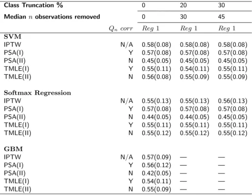
Table 1: Monte Carlo means and standard errors for different causal estimators that utilize the generalized propen-sity score. Data with a sample size of n = 500 were drawn from Data Generation Scenario 2 and 1,000 replicates were used. The true value for regimen 1 is E(Y1) = 0.55. SVM: Support Vector Machine; GBM: Generalized
Boosted Model; IPTW: Inverse Probability of Treatment Weighting; PSA: Propensity Score Adjustment; TMLE: Targeted Maximum Likelihood Estimation. Outcome regression models were fit by (I) regimen and (II) treatments as main terms covariates. Qn corr indicates whether the outcome model includes the true treatment-treatment
interactions.
Class Truncation % 0 20 30
Median n observations removed 0 30 45
Qncorr Reg 1 Reg 1 Reg 1
SVM IPTW N/A 0.58(0.08) 0.58(0.08) 0.58(0.08) PSA(I) Y 0.57(0.08) 0.57(0.08) 0.57(0.08) PSA(II) N 0.45(0.05) 0.45(0.05) 0.45(0.05) TMLE(I) Y 0.55(0.11) 0.54(0.11) 0.55(0.11) TMLE(II) N 0.56(0.08) 0.55(0.09) 0.55(0.09) Softmax Regression IPTW N/A 0.55(0.13) 0.55(0.13) 0.56(0.13) PSA(I) Y 0.57(0.08) 0.57(0.08) 0.57(0.08) PSA(II) N 0.44(0.05) 0.44(0.05) 0.45(0.05) TMLE(I) Y 0.55(0.11) 0.55(0.11) 0.55(0.11) TMLE(II) N 0.55(0.12) 0.55(0.12) 0.55(0.12) GBM IPTW N/A 0.57(0.09) — — PSA(I) Y 0.56(0.12) — — PSA(II) N 0.42(0.05) — — TMLE(I) Y 0.54(0.11) — — TMLE(II) N 0.55(0.09) — —
3. Summary statistics for the support of the regimens in the simulation studies
This section presents the tables for summary statistics and the plots for the supports for regimens 1 and 2 for simulation study I and regimen 1 for simulation study II, where simulation study I refers to the simulation study presented in Section 3 of the paper and simulation study II refers to the simulation study presented in Section 2 of the supplementary material. We define the “support” of a regimen to be the number of patients exposed to that regimen in the dataset.
Table 2: Summary Statistics for support for regimen 1 and regimen 2 for simulation study I.
n = 500 n = 1000
Reg 1 Reg 2 Reg 1 Reg 2
Minimum 68.00 29.00 147.00 74.00 1stQuantile 87.00 46.00 177.00 94.00 Median 92.00 51.00 185.00 101.00 Mean 92.48 51.04 184.90 100.90 3rd Quantile 98.00 56.00 193.00 107.00 Maximum 122.00 75.00 226.00 131.00
Table 3: Summary Statistics for support for regimen 1 for simulation study II with n = 500.
Reg 1 Minimum 16.00 1stQuantile 33.00 Median 37.00 Mean 36.75 3rdQuantile 41.00 Maximum 55.00
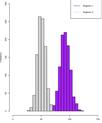
Figure 1: Histogram for the support of the top 2 regimens for Simulation Study I for n = 500.
Support Frequency 0 50 100 150 0 50 100 150 200 250 300 Regimen 1 Regimen 2
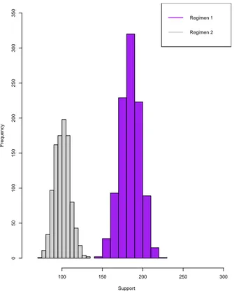
Figure 2: Histogram for the support of the top 2 regimens for Simulation Study I for n = 1000. Support Frequency 100 150 200 250 300 0 50 100 150 200 250 300 350 Regimen 1 Regimen 2
Figure 3: Histogram for the support of Regimen 1 for Simulation Study II for n = 500.
Support Frequency 0 20 40 60 80 100 0 50 100 150 200 250 300 350 Regimen 1
4. Summary Statistics for the weights obtained by the different estimating
meth-ods
This section contains the summary statistics of the weights obtained by SVM, Softmax Regression and GBM over 50 datasets for the regimens in simulation study I.
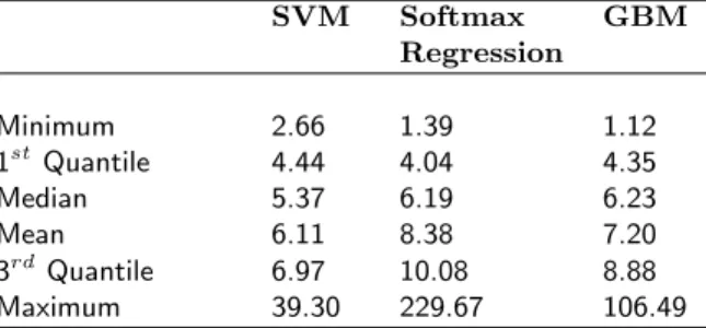
Table 4: Summary Statistics for the weights obtained by the different estimating methods for regimen 1 for simulation study I over 50 datasets with n = 1000.
SVM Softmax GBM Regression Minimum 2.66 1.39 1.12 1stQuantile 4.44 4.04 4.35 Median 5.37 6.19 6.23 Mean 6.11 8.38 7.20 3rdQuantile 6.97 10.08 8.88 Maximum 39.30 229.67 106.49
Table 5: Summary Statistics for the weights obtained by the different estimating methods for regimen 2 for simulation study I over 50 datasets with n = 1000.
SVM Softmax GBM Regression Minimum 3.09 1.44 1.05 1stQuantile 7.80 6.87 8.25 Median 11.08 12.99 13.73 Mean 13.11 23.98 17.06 3rdQuantile 16.27 26.93 21.33 Maximum 96.00 1163.50 544.76
5. Summary for the Generalized Propensity Scores for the MDR-TB Data
This section contains the summary of the truncated and the untruncated GPS obtained for the MDR-TB data using the different machine learning methods explained in Section 2.2. The GPS of the regimens are given by pi1 to pi10, where pi1 denotes GPS for Regimen 1 in our study and pi10 denotes the GPS for Regimen 10 in the study as mentioned in Section 4. The summary contains the following values:
• Min.: Minimum value of the GPS for the regimen in the sample study
• 1st Qu.: Value of the first quantile of the GPS for the regimen in the sample study • Median: Median value of the GPS for the regimen in the sample study
• Mean: Mean value of the GPS for the regimen in the sample study
• 3rd Qu.: Value of the third quantile of the GPS for the regimen in the sample study • Max.: Maximum value of the GPS for the regimen in the sample study
summary(Algorithm_Untruncated) denotes the summary of the untruncated GPS obtained using Algorithm whereas summary(Algorithm_Truncated) denotes the summary of the truncated GPS (20% truncation) obtained using Algorithm as mentioned in Section 4.
summary(SVM_Untruncated)
## pi1 pi2 pi3
## Min. :0.0000844 Min. :0.0001795 Min. :0.0000585 ## 1st Qu.:0.0003483 1st Qu.:0.0008688 1st Qu.:0.0007783 ## Median :0.0007693 Median :0.0016455 Median :0.0031000 ## Mean :0.1568600 Mean :0.0376882 Mean :0.0280186 ## 3rd Qu.:0.0084027 3rd Qu.:0.0056493 3rd Qu.:0.0157749 ## Max. :0.6704224 Max. :0.1603302 Max. :0.1602677
## pi4 pi5 pi6
## Min. :0.0000540 Min. :0.0000441 Min. :0.0004766 ## 1st Qu.:0.0005957 1st Qu.:0.0006334 1st Qu.:0.0020562 ## Median :0.0029060 Median :0.0014290 Median :0.0053386 ## Mean :0.0283911 Mean :0.0207455 Mean :0.0294543 ## 3rd Qu.:0.0282561 3rd Qu.:0.0025562 3rd Qu.:0.0256537 ## Max. :0.3174220 Max. :0.1382175 Max. :0.2802544
## pi7 pi8 pi9
## Min. :0.0001285 Min. :0.0002740 Min. :0.0000968 ## 1st Qu.:0.0005905 1st Qu.:0.0005881 1st Qu.:0.0009952 ## Median :0.0012020 Median :0.0011180 Median :0.0026187 ## Mean :0.0180373 Mean :0.0159779 Mean :0.0156337 ## 3rd Qu.:0.0049643 3rd Qu.:0.0019540 3rd Qu.:0.0054387 ## Max. :0.0815344 Max. :0.1821654 Max. :0.1104928
## pi10 ## Min. :0.0002061 ## 1st Qu.:0.0006178 ## Median :0.0008883 ## Mean :0.0133153 ## 3rd Qu.:0.0323348 ## Max. :0.0620212 summary(Softmax_Untruncated)
## pi1 pi2 pi3
## Min. :0.001606 Min. :0.001009 Min. :0.0009516 ## 1st Qu.:0.017372 1st Qu.:0.007144 1st Qu.:0.0085008
## Median :0.067361 Median :0.021264 Median :0.0225757 ## Mean :0.143315 Mean :0.039558 Mean :0.0366144 ## 3rd Qu.:0.192485 3rd Qu.:0.055097 3rd Qu.:0.0490858 ## Max. :0.673014 Max. :0.177946 Max. :0.1515242
## pi4 pi5 pi6
## Min. :0.001242 Min. :0.0006062 Min. :0.003809 ## 1st Qu.:0.005267 1st Qu.:0.0053993 1st Qu.:0.011288 ## Median :0.013764 Median :0.0150462 Median :0.018037 ## Mean :0.032116 Mean :0.0272295 Mean :0.025229 ## 3rd Qu.:0.029981 3rd Qu.:0.0373691 3rd Qu.:0.031908 ## Max. :0.298142 Max. :0.1224405 Max. :0.146441
## pi7 pi8 pi9
## Min. :0.0008831 Min. :0.0006065 Min. :0.0006481 ## 1st Qu.:0.0041477 1st Qu.:0.0061504 1st Qu.:0.0046522 ## Median :0.0123683 Median :0.0129524 Median :0.0124783 ## Mean :0.0193383 Mean :0.0212144 Mean :0.0219139 ## 3rd Qu.:0.0276799 3rd Qu.:0.0239001 3rd Qu.:0.0314892 ## Max. :0.0876790 Max. :0.1267092 Max. :0.0955858
## pi10 ## Min. :0.0004913 ## 1st Qu.:0.0048800 ## Median :0.0114627 ## Mean :0.0162796 ## 3rd Qu.:0.0284771 ## Max. :0.0625170 summary(GBM_Untruncated)
## pi1 pi2 pi3
## Min. :0.002027 Min. :0.0007163 Min. :0.007166 ## 1st Qu.:0.003807 1st Qu.:0.0009530 1st Qu.:0.007206 ## Median :0.006176 Median :0.0019908 Median :0.008290 ## Mean :0.168206 Mean :0.0404401 Mean :0.029222 ## 3rd Qu.:0.010221 3rd Qu.:0.0041522 3rd Qu.:0.010328 ## Max. :0.764830 Max. :0.3301783 Max. :0.179817
## pi4 pi5 pi6
## Min. :0.0000014 Min. :0.0000003 Min. :0.007889 ## 1st Qu.:0.0000777 1st Qu.:0.0000354 1st Qu.:0.012612 ## Median :0.0004492 Median :0.0003447 Median :0.013787 ## Mean :0.0263304 Mean :0.0232197 Mean :0.022999 ## 3rd Qu.:0.0167375 3rd Qu.:0.0005962 3rd Qu.:0.016079 ## Max. :0.9999966 Max. :0.3551773 Max. :0.307409
## pi7 pi8 pi9
## Min. :0.0009184 Min. :0.008467 Min. :0.0000007 ## 1st Qu.:0.0011354 1st Qu.:0.009411 1st Qu.:0.0000590 ## Median :0.0020279 Median :0.009560 Median :0.0004007 ## Mean :0.0197763 Mean :0.017003 Mean :0.0167759 ## 3rd Qu.:0.0038864 3rd Qu.:0.011996 3rd Qu.:0.0027138 ## Max. :0.1147831 Max. :0.053754 Max. :0.9586112
## pi10 ## Min. :0.0000003 ## 1st Qu.:0.0000269 ## Median :0.0000887 ## Mean :0.0152205 ## 3rd Qu.:0.0221909
## Max. :0.3435316 summary(SVM_Truncated)
## pi1 pi2 pi3
## Min. :0.0002831 Min. :0.0007573 Min. :0.0002799 ## 1st Qu.:0.0003483 1st Qu.:0.0008688 1st Qu.:0.0007783 ## Median :0.0007693 Median :0.0016455 Median :0.0031000 ## Mean :0.1568845 Mean :0.0377691 Mean :0.0280471 ## 3rd Qu.:0.0084027 3rd Qu.:0.0056493 3rd Qu.:0.0157749 ## Max. :0.6704224 Max. :0.1603302 Max. :0.1602677
## pi4 pi5 pi6
## Min. :0.0003056 Min. :0.0001582 Min. :0.001543 ## 1st Qu.:0.0005957 1st Qu.:0.0006334 1st Qu.:0.002056 ## Median :0.0029060 Median :0.0014290 Median :0.005339 ## Mean :0.0284244 Mean :0.0207595 Mean :0.029564 ## 3rd Qu.:0.0282561 3rd Qu.:0.0025562 3rd Qu.:0.025654 ## Max. :0.3174220 Max. :0.1382175 Max. :0.280254
## pi7 pi8 pi9
## Min. :0.0004759 Min. :0.0005308 Min. :0.0003049 ## 1st Qu.:0.0005905 1st Qu.:0.0005881 1st Qu.:0.0009952 ## Median :0.0012020 Median :0.0011180 Median :0.0026187 ## Mean :0.0180826 Mean :0.0159963 Mean :0.0156600 ## 3rd Qu.:0.0049643 3rd Qu.:0.0019540 3rd Qu.:0.0054387 ## Max. :0.0815344 Max. :0.1821654 Max. :0.1104928
## pi10 ## Min. :0.0005180 ## 1st Qu.:0.0006178 ## Median :0.0008883 ## Mean :0.0133594 ## 3rd Qu.:0.0323348 ## Max. :0.0620212 summary(Softmax_Truncated)
## pi1 pi2 pi3
## Min. :0.01423 Min. :0.005934 Min. :0.006702 ## 1st Qu.:0.01737 1st Qu.:0.007144 1st Qu.:0.008501 ## Median :0.06736 Median :0.021264 Median :0.022576 ## Mean :0.14408 Mean :0.039938 Mean :0.037119 ## 3rd Qu.:0.19248 3rd Qu.:0.055097 3rd Qu.:0.049086 ## Max. :0.67301 Max. :0.177946 Max. :0.151524
## pi4 pi5 pi6
## Min. :0.004416 Min. :0.004763 Min. :0.01005 ## 1st Qu.:0.005267 1st Qu.:0.005399 1st Qu.:0.01129 ## Median :0.013764 Median :0.015046 Median :0.01804 ## Mean :0.032373 Mean :0.027548 Mean :0.02563 ## 3rd Qu.:0.029981 3rd Qu.:0.037369 3rd Qu.:0.03191 ## Max. :0.298142 Max. :0.122440 Max. :0.14644
## pi7 pi8 pi9
## Min. :0.003598 Min. :0.005216 Min. :0.004309 ## 1st Qu.:0.004148 1st Qu.:0.006150 1st Qu.:0.004652 ## Median :0.012368 Median :0.012952 Median :0.012478 ## Mean :0.019558 Mean :0.021613 Mean :0.022207 ## 3rd Qu.:0.027680 3rd Qu.:0.023900 3rd Qu.:0.031489
## Max. :0.087679 Max. :0.126709 Max. :0.095586 ## pi10 ## Min. :0.003998 ## 1st Qu.:0.004880 ## Median :0.011463 ## Mean :0.016521 ## 3rd Qu.:0.028477 ## Max. :0.062517 summary(GBM_Truncated)
## pi1 pi2 pi3
## Min. :0.003807 Min. :0.0009182 Min. :0.007206 ## 1st Qu.:0.003807 1st Qu.:0.0009530 1st Qu.:0.007206 ## Median :0.006176 Median :0.0019908 Median :0.008290 ## Mean :0.168406 Mean :0.0404581 Mean :0.029225 ## 3rd Qu.:0.010221 3rd Qu.:0.0041522 3rd Qu.:0.010328 ## Max. :0.764830 Max. :0.3301783 Max. :0.179817
## pi4 pi5 pi6
## Min. :0.0000389 Min. :0.0000300 Min. :0.01138 ## 1st Qu.:0.0000777 1st Qu.:0.0000354 1st Qu.:0.01261 ## Median :0.0004492 Median :0.0003447 Median :0.01379 ## Mean :0.0263347 Mean :0.0232217 Mean :0.02349 ## 3rd Qu.:0.0167375 3rd Qu.:0.0005962 3rd Qu.:0.01608 ## Max. :0.9999966 Max. :0.3551773 Max. :0.30741
## pi7 pi8 pi9
## Min. :0.001127 Min. :0.009411 Min. :0.0000432 ## 1st Qu.:0.001135 1st Qu.:0.009411 1st Qu.:0.0000590 ## Median :0.002028 Median :0.009560 Median :0.0004007 ## Mean :0.019807 Mean :0.017013 Mean :0.0167803 ## 3rd Qu.:0.003886 3rd Qu.:0.011996 3rd Qu.:0.0027138 ## Max. :0.114783 Max. :0.053754 Max. :0.9586112
## pi10 ## Min. :0.0000189 ## 1st Qu.:0.0000269 ## Median :0.0000887 ## Mean :0.0152223 ## 3rd Qu.:0.0221909 ## Max. :0.3435316
6. Tables for the Probability estimates of treatment success of the truncated
GPS(20% truncation) as mentioned in Section 4 for MDR-TB data
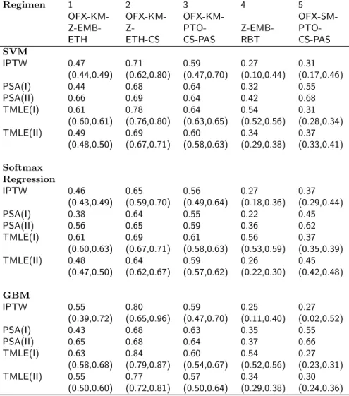
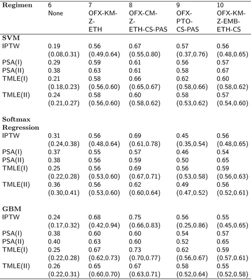
In a sensitivity analysis, 20% truncation was used to remove the smallest values of the Generalized Propensity Score for the top 10 available regimens. The point estimates of E(Yr) and the confidence intervals for the
top 10 regimens are presented in Table 6 and 7. The GPS truncation resulted in at most small changes in the point estimates as opposed to the results obtained without the truncation of GPS and had similar conclusions to it.
Table 6: Estimates of the probability of treatment success along with the confidence intervals under regimens 1-5 for the MDR-TB application in Section 4 after 20% truncation of the GPS. SVM: Support Vector Machine; GBM: Generalized Boosted Model; IPTW: Inverse Probability of Treatment Weighting; PSA: Propensity Score Adjustment; TMLE: Targeted Maximum Likelihood Estimation. Outcome regression models were fit by (I) regimen and (II) treatments as main terms covariates.
Regimen 1 2 3 4 5
OFX-KM- OFX-KM- OFX-KM-
OFX-SM-Z-EMB- Z- PTO- Z-EMB-
PTO-ETH ETH-CS CS-PAS RBT CS-PAS
SVM IPTW 0.47 0.71 0.59 0.27 0.31 (0.44,0.49) (0.62,0.80) (0.47,0.70) (0.10,0.44) (0.17,0.46) PSA(I) 0.44 0.68 0.64 0.32 0.55 PSA(II) 0.66 0.69 0.64 0.42 0.68 TMLE(I) 0.61 0.78 0.64 0.54 0.31 (0.60,0.61) (0.76,0.80) (0.63,0.65) (0.52,0.56) (0.28,0.34) TMLE(II) 0.49 0.69 0.60 0.34 0.37 (0.48,0.50) (0.67,0.71) (0.58,0.63) (0.29,0.38) (0.33,0.41) Softmax Regression IPTW 0.46 0.65 0.56 0.27 0.37 (0.43,0.49) (0.59,0.70) (0.49,0.64) (0.18,0.36) (0.29,0.44) PSA(I) 0.38 0.64 0.55 0.22 0.45 PSA(II) 0.56 0.65 0.59 0.36 0.62 TMLE(I) 0.61 0.69 0.61 0.56 0.37 (0.60,0.63) (0.67,0.71) (0.58,0.63) (0.53,0.59) (0.35,0.39) TMLE(II) 0.48 0.64 0.59 0.26 0.45 (0.47,0.50) (0.62,0.67) (0.57,0.62) (0.22,0.30) (0.42,0.48) GBM IPTW 0.55 0.80 0.59 0.25 0.27 (0.39,0.72) (0.65,0.96) (0.47,0.70) (0.11,0.40) (0.02,0.52) PSA(I) 0.43 0.68 0.63 0.35 0.55 PSA(II) 0.65 0.68 0.64 0.37 0.66 TMLE(I) 0.63 0.84 0.60 0.54 0.27 (0.58,0.68) (0.79,0.87) (0.54,0.67) (0.52,0.56) (0.23,0.31) TMLE(II) 0.55 0.77 0.57 0.34 0.30 (0.50,0.60) (0.72,0.81) (0.50,0.64) (0.29,0.38) (0.24,0.36)
Table 7: Estimates of the probability of treatment success along with the confidence intervals under regimens 6-10 for the MDR-TB application in Section 4 after 20% truncation of the GPS. SVM: Support Vector Machine; GBM: Generalized Boosted Model; IPTW: Inverse Probability of Treatment Weighting; PSA: Propensity Score Adjustment; TMLE: Targeted Maximum Likelihood Estimation. Outcome regression models were fit by (I) regimen and (II) treatments as main terms covariates.
Regimen 6 7 8 9 10
None OFX-KM- OFX-CM- OFX-
OFX-KM-Z- Z- PTO-
Z-EMB-ETH ETH-CS-PAS CS-PAS ETH-CS
SVM IPTW 0.19 0.56 0.67 0.57 0.56 (0.08,0.31) (0.49,0.64) (0.55,0.80) (0.37,0.76) (0.48,0.65) PSA(I) 0.29 0.59 0.61 0.56 0.57 PSA(II) 0.38 0.63 0.61 0.58 0.67 TMLE(I) 0.21 0.58 0.66 0.62 0.60 (0.18,0.23) (0.56,0.60) (0.65,0.67) (0.58,0.66) (0.58,0.62) TMLE(II) 0.24 0.58 0.60 0.58 0.57 (0.21,0.27) (0.56,0.60) (0.58,0.62) (0.53,0.62) (0.54,0.60) Softmax Regression IPTW 0.31 0.56 0.69 0.45 0.56 (0.24,0.38) (0.48,0.64) (0.61,0.78) (0.35,0.54) (0.48,0.65) PSA(I) 0.37 0.55 0.57 0.46 0.54 PSA(II) 0.38 0.56 0.59 0.50 0.65 TMLE(I) 0.25 0.56 0.69 0.56 0.59 (0.22,0.28) (0.53,0.60) (0.67,0.71) (0.53,0.58) (0.56,0.63) TMLE(II) 0.36 0.56 0.62 0.49 0.56 (0.30,0.41) (0.53,0.60) (0.60,0.64) (0.47,0.52) (0.52,0.61) GBM IPTW 0.24 0.68 0.75 0.56 0.55 (0.17,0.32) (0.42,0.94) (0.66,0.83) (0.25,0.86) (0.45,0.65) PSA(I) 0.38 0.60 0.60 0.54 0.57 PSA(II) 0.40 0.63 0.60 0.52 0.65 TMLE(I) 0.25 0.67 0.73 0.62 0.59 (0.22,0.28) (0.62,0.73) (0.70,0.77) (0.56,0.67) (0.57,0.61) TMLE(II) 0.26 0.65 0.67 0.58 0.55 (0.22,0.31) (0.60,0.70) (0.63,0.71) (0.52,0.64) (0.52,0.58)