Effects of small-scale atmospheric activity on precise positioning

Contract ref : GJU/06/2423/CTR/GALOCAD G. Wautelet, S. Lejeune, S. Stankov, H. Brenot, R. Warnant Verified by : R. Warnant

GALOCAD

Development of a Galileo Local Component for the nowcasting

and forecasting of atmospheric disturbances affecting the

integrity of high precision Galileo applications.

WP 230 Technical Report:

“Effects of small-scale atmospheric activity on precise

positioning”

LIST OF ABBREVIATIONS

BDN Belgian Dense Network

GI/BAS Geophysical Institute of the Bulgarian Academy of Sciences GNSS Global Navigation Satellite System

GPS Global Positioning System

HDK Hybrid Dourbes K model

IMF Interplanetary Magnetic Field

Kd K index for Dourbes (Belgium)

MAK Muhtarov Andonov Kutiev model for forecasting Dourbes K

NWP Numerical Weather Prediction models

RINEX Receiver Independent Exchange format

RMI Royal Meteorological Institute

ROB Royal Observatory of Belgium

RTK Real Time Kinematics

TEC Total Electron Content

TECU TEC Unit

TID Travelling Ionospheric Disturbance

WEM Weighted Extrapolation Model

WP Work Package

TABLE OF CONTENT

List of abbreviations………2

Table of Content……….………...3

1. Introduction………..4

2. Atmospheric effects on RTK ……….………...5

3. Methodology to assess atmospheric effects on RTK….. ………....7

4. Quantitative study of the positioning error due to the ionosphere……….10

5. Correlation between ionospheric residual term and positioning error………...18

6. Quantitative study of the positioning error due to the neutral atmosphere...………….28

7. Ionospheric effects on aviation….……….33

8. Conclusions………48

1 INTRODUCTION

Nowadays, Global Navigation Satellite Systems or GNSS allow to measure positions in real time with an accuracy ranging from a few meters to a few centimetres mainly depending on the type of observable (code or phase measurements) and on the positioning mode used (absolute, differential or relative). In absolute mode, the observer measures his absolute position with only one receiver; the differential mode is a particular case of the absolute mode: the observer still wants to measure his absolute position with only one receiver but he makes use of differential corrections broadcast by a reference station. These corrections allow improving the quality of the measured positions. In relative mode, the observer combines the measurements collected by at least two receivers. The absolute position of one of these two receivers (called reference receiver or reference station) must be known. Based on the combined measurements, it is possible to compute the vector (often called baseline) between the two receivers. Then, the absolute position of the second receiver can be obtained.

The best accuracies can be reached in differential or relative mode using phase measurements. For example, the so-called Real Time Kinematic technique (RTK) allows to measure positions in real time with accuracy usually better than a decimetre. RTK can be used in both differential and relative modes. The level of accuracy obtained mainly depends on the distance between the reference station and the mobile user of whom the position is unknown. Indeed, the RTK technique makes the assumption that the phase measurements made at the reference station and by the mobile user are affected in the same way by most of the error sources: satellite clock and orbit errors, atmospheric effects. In practice, the distance between the reference station and the user is usually smaller than 20 km.

At the present time, atmospheric effects remain the most important error source in high accuracy positioning with the RTK technique. In particular, small-scale variability mainly in the ionospheric plasma but also in the neutral atmosphere can be the origin of strong degradations of RTK accuracy. In the past, many studies have been dedicated to atmospheric effects on real time positioning techniques. Most of them aimed at developing mitigation techniques which allow improving the precision obtained on short distances or aimed at increasing the “acceptable” distance between the stations considered while minimizing the errors. In this report, we develop a method allowing to assess the positioning error which is due to residual atmospheric effects remaining when the mitigation techniques have been applied to the data. The method developed in the frame of this project, does not aim at improving the precision obtained in RTK positioning but it allows to monitor and to quantify the contribution of atmospheric disturbances to the RTK technique error budget.

Applications in aviation are based on carrier-smoothed code observables and also use differential corrections. Therefore, small-scale structures in the ionosphere can also pose a threat for such critical applications. In section 7, we analyze local TEC behaviour induced by the storm of November 20 2003 which could degrade the quality of differential corrections provided by a reference station to an aircraft.

2 ATMOSPHERIC EFFECTS ON RTK

As already stated, the RTK technique can be run both in differential and in relative mode. To fix ideas, we choose to discuss ionospheric effects on RTK used in relative mode: atmospheric disturbances have a similar influence on both positioning modes.

In relative mode, RTK users combine their own phase measurements with the measurements made by a reference station of which the position is precisely known. In practice, the mobile user forms double differences between its own phase measurements and the phase measurements collected in the reference station. In this report, we call receiver A, the reference station receiver, and receiver B, the user receiver.

The simplified mathematical model of phase measurements made by receiver A on satellite i, i_,

A k

ϕ (in cycles of carrier k = L1 or L2) can be written as follows (Seeber (2003); Leick (2004)): i_, k

(

(

)

)

, the geometric distance (m) between receiver A and satellite i ;

I , the ionospheric error (m) on carrier k;

i A

T , the tropospheric error (m);

A t Δ i t Δ , i A k N , i

, the receiver clock error (the synchronisation error of the receiver time scale with respect to GPS time scale, in seconds) ;

, the satellite clock synchronisation error (the synchronisation error of the satellite time scale with respect to GPS time scale, in seconds) ;

, the phase ambiguity on carrier k (integer number) ;

A k

M , multipath effect (m) on carrier k ; ,

i A k

ε , noise (cycles) on carrier k ;

k

f , the considered carrier frequency (Hz). If we neglect higher order terms (terms in 3

k

f − , f_k−4…), the ionospheric error I_{A k}i_, is

given by: i_, 40.3 ₂ i A A k I k TEC f = (2.2) with: i A

If i_, A k

ϕ and are phase measurements made simultaneously by receivers A and B on satellite i, the single difference is defined as:

, i B k ϕ , i AB k ϕ i _, i_, , i AB k=ϕA k−ϕB k (2.3) ϕ

If receivers A and B observe a second common satellite j, we can form a second single difference j _,

AB k

ϕ . Then, the double difference i j_, AB k ϕ is defined as: _, i _, j (2.4) k AB k AB k ϕi j =ϕ −ϕ AB ,

Based on equation (2.1), equation (2.4) can be rewritten:

i j_,

(

)

i j ( i_, ) ( j_, j_, (2.6)

AB ∗ − ∗k B k − ∗ − ∗A k B k

In double differences, all the error sources which are common to the phase measurements performed by receivers A and B cancel, in particular, satellite and receiver clock errors. In addition, in the case of RTK, which is used on short distances, orbit residual errors can be neglected (Seeber, 2003). Indeed, we can compute the ephemeris accuracy needed to measure a baseline of 20 km (maximal acceptable distance in RTK) with an accuracy of 1 cm by using the following formula (Leick 2004):

i AB i AB A dR db b = R (2.7) with :

- dbAB and dRi respectively the error on the baseline length and the error on satellite

i position (orbit error) ;

- bAB and RAi respectively the baseline vector and the vector linking the satellite i

and the receiver A.

If we consider a typical range of 22 000 km between the satellite and the receiver (Ri A),

we find a required ephemeris accuracy of about 11 m. This means that we need satellite positions with accuracy better than 11 m to measure a 20km baseline with 1 cm accuracy. Nowadays, broadcast ephemeris accuracy is about 1.6 m (cf. IGS website); therefore, the orbit residual error can be neglected with respect to the nominal RTK accuracy (which usually ranges between a few cm to about a decimetre for baselines smaller than 10-15 km.

Residual atmospheric effects i j AB

T and I_{AB k}i j_, depend on the distance between stations A

and B and also on the atmospheric “activity”. Given the short distances considered, RTK data processing algorithms assume that residual atmospheric errors are negligible. In this case, neglecting multipath and noise, equation (2.5) can be rewritten:

i j_, k i j i j , AB k AB AB k f D N c ϕ = + (2.8) For the ease of reading, we shall omit the subscript “k” when it is not necessary in the discussion.

In RTK, the position of the reference station (station A) is known by the mobile user (station B). For this reason, the only unknowns which remain in equation (2.8) are the mobile user coordinates XB, YB, ZB (contained in the term D_ABi j ) and the ambiguity N_ABi j

which is an integer number. Let’s assume that five (common) satellites (satellites 1,2,3,4,5) are observed in stations A and B: four independent double differences can be formed 12 AB ϕ , 13 AB ϕ , 14 AB ϕ , 15 AB

ϕ . These four equations contain seven unknowns: XB, YB, ZB, 12

AB

N , N_AB13, N_AB14, N_AB15. Therefore, it is not possible to solve all the unknowns using only one observation epoch: RTK needs an initialisation phase. During the initialisation phase, the user remains at the same position during a few minutes so that redundant observations and sufficient information are available to solve (by least squares) the linearised double difference observations for the ambiguities and for the user position. Precise positioning with RTK requires the resolution of the ambiguities i j

AB

N to the correct integer value in real-time. The ambiguity resolution requires the use of sophisticated techniques like the so-called LAMBDA method (Joosten & Tiberius, 2000). When ambiguities are solved, the user can start to measure precise positions. Equation (2.8) remains a valid mathematical model for double differences as long as residual atmospheric errors remain negligible with respect to GPS carrier wavelength (about 20 cm). This assumption is verified in usual conditions (Leick, 2004). In practice, disturbed meteorological and/or Space Weather conditions can be the origin of small-scale (a few kilometres) atmospheric variability which can itself strongly degrade or even prevent ambiguity resolution due to the fact that, in that case, the mathematical model given by equation (2.8) does not adequately represent the observed double differences.

The meteorological and Space Weather conditions which are the origin of the occurrence of small-scale structures in the atmosphere have been characterized in details in WP 250 and WP 220 reports.

3 METHODOLOGY TO ASSESS ATMOSPHERIC EFFECTS ON RTK

In order to have a realistic quantitative assessment of the ionospheric influence on RTK accuracy, we decided to develop software based on the technique used in RTK to compute real time positions on the field. This technique has been described in paragraph 2. The idea is to reproduce as close as possible the “positioning conditions” that RTK

users undergo on the field. Nevertheless, it is very clear that each observation site is different and that it will never be possible to reproduce exactly the conditions encountered by each user. This software uses GPS stations from the Belgian Dense Network to play the role of reference station (station A) and mobile station (station B). The position of these stations is known at a few mm level. As the “nominal” RTK accuracy is a few cm, we will consider that the position of these permanent stations is perfectly known and we will refer to it as the “true” station position.

The most difficult point is to be able to isolate the part of the user position error budget which is due only to the ionosphere or to the neutral atmosphere. In order to achieve this goal, data are processed in 5 steps.

3.1.

Resolution of L1 and L2 ambiguities and computation of the term

GF AB

I _,

In WP 220 paragraph 5, we have outlined the strategy we are using to compute i j AB

TEC (which allows to obtain i j_,

AB k

I ) and to solve the L1 and L2 double difference integer

ambiguities i j_, AB k

N . The same strategy is applied here. During this step, our software

forms double differences based on the L1 and L2 phase measurements collected on all the satellites in view in stations A and B. Then ambiguities i j_{, 1}

AB L

N and N_{AB L}i j_{, 2} are solved

based on double differences of the wide lane and of the geometric free combinations; these ambiguities are not solved on periods of a few minutes as it is the case “on the field” but using all the available data for the considered satellite pair. When the ambiguities are solved, the term i j

AB

TEC can be computed from double differences of the geometric free combination neglecting multipath and noise (see WP 220 report equations 5.6 and 5.8): 16 , , 0,552 10 , i j i j i j i j i j , AB GF NAB GF TECAB MAB GF AB GF ϕ _{− =} − _{+ +}ε _(3.1) Then i j_, AB k

I can be obtained from TEC_ABi j :

_, 40.3 ₂ i j i j AB AB k k TEC I f = (3.2) Let’s underline that, in practice, the term i j_,

AB k

I obtained by this method also contains the

3.2. Computation of the user position (station B)

The user position can be computed from the linearised equation (2.5) where it is assumed that all error terms ( i j

AB

T , i j_, AB k

I , i j_, AB k

M ) are negligible and where double differences are

corrected for the ambiguity (solved during step 1):

i j_, i j_, k

(

)

The position is obtained from a least square adjustment involving 5 minute periods of measurements. In practice, the positions computed during this step are still affected by all error terms. We shall refer to these positions as: XB,1 , YB,1 , ZB,1.

3.3. Computation of the user position based on double difference corrected

for the ionospheric effect

Double differences i j_, AB k

ϕ are corrected for the ambiguity and for the ionospheric term

,

i j AB k

I obtained during step 1:

i j_, k i j_, i j_, k

(

)

The user position can be computed again from these double differences corrected for the ionosphere (equation (3.4)) where it is assumed that all remaining error terms ( i j

AB

T ,M_{AB k}i j_, ) are negligible. In a similar way as it has been done in step 2, the position is

obtained from a least square adjustment involving 5 minute periods of measurements. We shall refer to these positions as: XB,2 , YB,2 , ZB,2. From equation (3.4), we see that they do

not depend on the ionospheric effects but they still depend on i j AB

T , , noise and also

on satellite geometry. In fact, taking into account the way it is computed, the term

, i j AB k M , i j AB k I

also contains multipath. Therefore, we can consider that these double differences corrected for i j_,

AB k

I are also corrected for (a part of) multipath. Nevertheless, as the

magnitude of ionospheric effects is usually much larger than the magnitude of multipath, we shall consider that the difference between (XB,1 , YB,1 , ZB,1) and (XB,2 , YB,2 , ZB,2) is

mainly due to the ionosphere.

3.4. Computation of the positioning error due to the ionosphere

The absolute value of the difference between (XB,1 , YB,1 , ZB,1) and (XB,2 , YB,2 , ZB,2) is

positions. Indeed, it allows to “isolate” the influence of the ionosphere from the other error sources. This difference can be transformed into horizontal and vertical components (north, east, up) and will be referred to as (ΔNiono, ΔEiono, ΔUiono).

3.5. Computation of the positioning error due to the troposphere

From the discussion above, it comes that (XB,2 , YB,2 , ZB,2) still depends on tropospheric

effects, geometry, residual multipath and noise. Therefore, we shall assess the influence of the troposphere on RTK positions by computing the absolute value of the difference between the “true” position and the computed position (XB,2 , YB,2 , ZB,2). Nevertheless, it

is important to underline that this strategy has a disadvantage: not only disturbed tropospheric conditions can be the origin of large differences between these positions; for example, bad satellite coverage could also be the origin of “out of tolerance” errors. We will have to take this point into account during our discussion about tropospheric effects.

4 QUANTITATIVE STUDY OF THE POSITIONING ERROR DUE TO THE IONOSPHERE

4.1. Presentation of the cases studies and methodology

In this paragraph, we will analyse the same cases than in WP 220: 5 baselines and 4 different days. The baselines are the following ones (figure 4.1):

• GILL – LEEU (11.3 km) • GILL – MECH (20.5 km) • OUDE – GERA (19.9km) • OUDE – ZVEW (19.4 km) • OUDE – GENT (18.7 km) The selected days for the analysis are:

• Quiet day: 103/07 ;

• Day with medium-amplitude TID: 359/04, satellite pair 5/6 (9.725h – 9.966h) ; • Day with large-amplitude TID: 301/03, satellite pair 7/5 (11.33h – 11.575h) ; • Day with severe geomagnetic storm: 324/03, satellite pair 16/2 (17.358h –

17.608h).

Let us recall that the periods described above were chosen on the basis of the results obtained from the one-station method. Indeed, these selected periods correspond to time intervals where RoTEC values and variability (for a given satellite) were representative of the “typical cases” we wanted to analyze: quiet ionosphere, TID or geomagnetic storm.

In WP 220, these periods have been processed and analyzed with the double difference software in order to quantify the effects of the residual ionosphere on specific satellite pairs during these typical ionospheric conditions. The outputs of this analysis were values of the ionospheric residual term related to given satellite pairs.

In this section, the goal is to assess the influence of these specific double differences in terms of positioning error. As the least-square process needs at least 3 different satellite pairs to compute the positioning error (if the ambiguities are solved), we can not affirm that those analyzed periods, which correspond to typical cases in terms of RoTEC, induce automatically the worst positioning error values for the whole considered day. Indeed, the other satellite pairs involved in the least-square process could be less “affected” by the ionospheric effects.

Figure 4.1. Selected baselines

As explained in section 3, the positioning error due to the ionosphere (ΔNiono, ΔEiono,

ΔUiono) is computed on 5 minute periods. For each 15 minute interval, we obtain only 3

positioning errors per baseline, which is too few to make Fisher’s test like in WP 220 to assess the influence of the baseline length or orientation on the positioning error due to ionospheric residual term. However, we will extract some quantitative statistics about the positioning error to assess of the error distribution among the different baselines.

4.2. Quiet day: 103/07

In order to characterize a quiet ionospheric day, we have chosen to use the 288 positioning errors (ΔNiono, ΔEiono, ΔUiono) relative to the 24 hours of the day (periods of 5

minutes).

We compute the mean and the standard deviation for each baseline and each component; these values expressed in meters are shown in table 1.

North East Up

Mean Sd Mean Sd Mean Sd

[m] [m] [m] [m] [m] [m] GILL - LEEU 0.0051 0.0035 0.0032 0.0022 0.0068 0.0060 GILL - MECH 0.0061 0.0048 0.0029 0.0023 0.0085 0.0072 OUDE - GERA 0.0069 0.0067 0.0050 0.0043 0.0100 0.0099 OUDE - ZWEV 0.0048 0.0045 0.0053 0.0038 0.0090 0.0081 OUDE - GENT 0.0080 0.0055 0.0030 0.0030 0.0082 0.0067

Table 1. Positioning error due to the ionosphere considering 24h of data; quiet day in terms of ionospheric variability (DOY 103/07).

Table 1 allows us to quantify the “nominal” positioning error due to the ionosphere on a given baseline; as we have four baselines having a similar length (GILL-MECH, OUDE-GERA, OUDE-ZWEV and OUDE-GENT), we can compute the mean of the positioning error to quantify the effect of the ionospheric residual error during a quiet ionospheric day. Moreover, we can extract from these four 20 km baselines the maximum and minimum values of the positioning error due to the ionosphere for each of the three components (table 2). North East Up [m] [m] [m] Mean 0.0064 0.0040 0.0089 Min 0.0000 0.0000 0.0000 Max 0.0299 0.0260 0.0545

Table 2. Mean, minimum and maximum of the positioning error due to the ionosphere for the four 20 km baselines (DOY 103/07).

The analysis of table 2 shows that the mean positioning error due to the ionosphere ranges from about 4 to 9 mm for a 20 km baseline, depending on the considered component. Maximum positioning errors range from about 25 mm to 55 mm; these values are not “out of tolerance” with respect to the typical accuracy of the RTK technique. Indeed, we consider that RTK allows to measure positions with an accuracy ranging from a few centimetres to about a decimetre during standard conditions for baselines smaller than 10-15 km.

In conclusions, tables 1 & 2 show that positioning error due to the ionosphere for a 20 km baseline is less than 1 cm on average but can reach more that 5 cm.

4.3. Day with medium-amplitude TID: 359/04

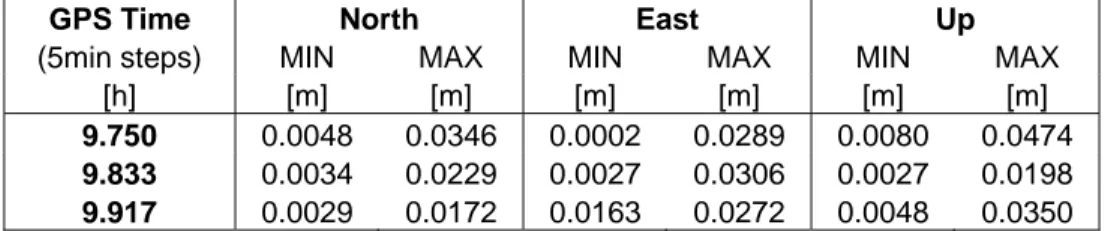
The selected 15 minute interval where the TID occurred allows us to extract the positioning error due to the ionosphere every 5 minutes for each of the components; the results are shown in table 3.

By comparing the values shown in table 3 with the values relative to the quiet day (see tables 1 & 2), we can say that a major part of the positioning errors during the occurrence of this TID is larger than the mean positioning error observed during the quiet day 103/07. From table 3, we can also say that the TID of DOY 359/04 induces a positioning error which is distributed on each component during the least-square process.

GPS Time North East Up

(5min steps) [h] [m] [m] [m] 9.750 0.0024 0.0158 0.0135 GILL – LEEU 9.833 0.0155 0.0026 0.0124 9.917 0.0108 0.0133 0.0078 9.750 0.0117 0.0059 0.0474 GILL – MECH 9.833 0.0070 0.0027 0.0198 9.917 0.0102 0.0196 0.0065 9.750 0.0134 0.0047 0.0267 OUDE - GERA 9.833 0.0034 0.0088 0.0027 9.917 0.0029 0.0163 0.0131 9.750 0.0048 0.0002 0.0080 OUDE - ZWEV 9.833 0.0168 0.0306 0.0185 9.917 0.0172 0.0187 0.0048 9.750 0.0346 0.0289 0.0200 OUDE – GENT 9.833 0.0229 0.0044 0.0112 9.917 0.0114 0.0272 0.0350

Table 3. Positioning error due to the ionosphere during the TID of DOY 359/04.

Moreover, the analysis of table 3 shows that, for a similar baseline orientation (i.e. GILL-LEEU and GILL-MECH baselines), we cannot state that the positioning error due to the occurrence of the TID is smaller for the smaller baseline than for the other one. Let us recall that table 3 contains results obtained during a 15 minute period, which is not necessarily representative of the positioning error experienced during the whole day. Further investigations and more data are necessary to establish a relationship between the baseline length and the positioning error due to the ionosphere (see section 5).

Nevertheless, considering the four baselines of about 20 km length, we can compute the descriptive statistics that are the mean, the minimum and the maximum of the positioning error for each of the five minute interval (tables 4 & 5).

Table 5 shows that for the same time interval and the same component, the positioning errors can be very different from a baseline to another because minimum and maximum values are very far from each other. For example, during the time interval of 9.750 h, the positioning error on the north component ranges between 5 mm and 35 mm, depending on the considered baseline.

GPS Time North East Up

(5min steps)

[h] [m] [m] [m]

9.750 0.0162 0.0099 0.0255

9.833 0.0100 0.0093 0.0104

9.917 0.0104 0.0205 0.0148

Table 4. Mean of the positioning error due to the ionosphere on the four 20 km baselines during the occurrence of the TID of DOY 359/04.

GPS Time North East Up

(5min steps) MIN MAX MIN MAX MIN MAX

[h] [m] [m] [m] [m] [m] [m]

9.750 0.0048 0.0346 0.0002 0.0289 0.0080 0.0474 9.833 0.0034 0.0229 0.0027 0.0306 0.0027 0.0198 9.917 0.0029 0.0172 0.0163 0.0272 0.0048 0.0350

Table 5. Maximum and minimum positioning errors due to the ionosphere on the four 20 km baselines during the occurrence of the TID of DOY 359/04.

Finally, the effects of the medium-amplitude TID of DOY 359/04 on positioning error due to the ionosphere seem to depend mainly on baseline orientation and on the considered component. The observed positioning error due to ionosphere ranges between less than 1 mm and about 5 cm. The maximum error due to the medium-amplitude TID on DOY 359/04 during the considered 15 minute time interval is of the same order of magnitude than the maximum error experienced during the quiet day. Therefore, further investigation based on more data is necessary (see section 5).

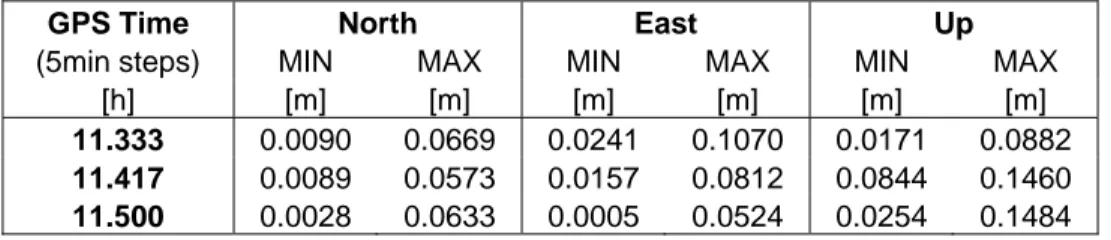
4.4. Day with large-amplitude TID: 301/03

We can use the same reasoning than for the section 4.3 to analyze the effect of a large-amplitude TID on the positioning error due to the ionosphere (table 6).

GPS Time North East Up (5min steps) [h] [m] [m] [m] 11.333 0.0296 0.0346 0.0246 GILL - LEEU 11.417 0.0466 0.0002 0.0193 11.500 0.0436 0.0073 0.0280 11.333 0.0134 0.1070 0.0171 GILL - MECH 11.417 0.0573 0.0354 0.0844 11.500 0.0633 0.0005 0.1484 11.333 0.0539 0.0272 0.0390 OUDE - GERA 11.417 0.0089 0.0812 0.1460 11.500 0.0028 0.0524 0.0414 11.333 0.0669 0.0241 0.0574 OUDE - ZWEV 11.417 0.0227 0.0530 0.1155 11.500 0.0215 0.0018 0.0423 11.333 0.0090 0.0384 0.0882 OUDE - GENT 11.417 0.0209 0.0157 0.0852 11.500 0.0335 0.0379 0.0254

Table 6. Positioning error due to the ionosphere during the TID of DOY 301/03.

As for the day 359/04, we can also compute the mean, the maximum and minimum values of the positioning error for each time period and each component for the four baselines considered (tables 7 & 8).

GPS Time North East Up

(5min steps)

[h] [m] [m] [m]

11.333 0.0358 0.0492 0.0504 11.417 0.0219 0.0370 0.0862 11.500 0.0303 0.0232 0.0644

Table 7. Mean of the positioning error due to the ionosphere on the four 20 km baselines during the occurrence of the TID of DOY 301/03.

GPS Time North East Up

(5min steps) MIN MAX MIN MAX MIN MAX

[h] [m] [m] [m] [m] [m] [m]

11.333 0.0090 0.0669 0.0241 0.1070 0.0171 0.0882 11.417 0.0089 0.0573 0.0157 0.0812 0.0844 0.1460 11.500 0.0028 0.0633 0.0005 0.0524 0.0254 0.1484

Table 8. Maximum and minimum positioning errors due to the ionosphere on the four 20 km baselines during the occurrence of the TID of DOY 301/03.

When considering the results shown in tables 6 to 8 and by following the same reasoning than in section 4.3 to analyze the data, the conclusions are quite similar than in the case of the medium-amplitude TID:

• Baseline length does not seem to have an influence on the magnitude of the positioning error due to the ionosphere. Indeed, the positioning error values are sometimes smaller and sometimes larger for the smaller baseline GILL-LEEU (11.3 km). This effect could be due to the physical properties of the TID (wavelength, speed, spatial extent…).

• The positioning error fluctuates very strongly from a component to another. • The positioning error fluctuates very strongly from a baseline to another.

Nevertheless, we can say that the mean and the maximum values are larger for the large-amplitude TID (around 15 cm) than for the medium-large-amplitude TID (around 5 cm) and for the quiet day (around 5 cm). Indeed, when having a look at tables 4, 5, 7 & 8 we clearly see that mean and standard deviation values are larger during the occurrence of the large-amplitude TID.

Finally, we can conclude that during the occurrence of the TID of DOY301/03, the positioning error due to the ionosphere ranges between less than 1 mm and about 15 cm.

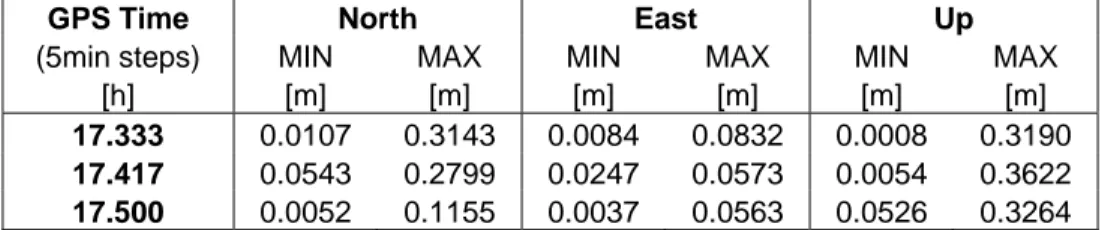
4.5. Day with geomagnetic storm: 324/03

As in section 4.4, we use the same methodology to assess the effects of a severe geomagnetic storm on the positioning error due to the ionosphere (tables 9 to 11).

The conclusions that we can formulate on the basis of tables 9 to 11 are also the same as for the previous sections (see sections 4.3 & 4.4).

However, the smaller baseline GILL-LEEU (11.3 km) seems to be a little less disturbed than the baseline GILL-MECH (20.5 km) which has the same orientation. Indeed, from table 9 we can observe that nearly all values of the positioning error are larger for the 20 km baseline than for the 11 km baseline. Nevertheless, we need to analyze more data to confirm the assumption that, in case of geomagnetic storm, the positioning error induced by the ionosphere increases with increasing baseline length (see section 5).

Tables 10 & 11 allow us to quantify the positioning error for a typical 20 km baseline. We can see that these values are generally larger than the values obtained for the DOY 301/03 (tables 7 & 8) and, a fortiori, than the values of DOY 359/04 and 103/07.

GPS Time North East Up (5min steps) [h] [m] [m] [m] 17.333 0.0392 0.0048 0.0127 GILL - LEEU 17.417 0.0690 0.0091 0.0540 17.500 0.0006 0.0795 0.0264 17.333 0.3143 0.0469 0.3190 GILL - MECH 17.417 0.2799 0.0247 0.3622 17.500 0.0052 0.0099 0.0526 17.333 0.1130 0.0257 0.1728 OUDE - GERA 17.417 0.1893 0.0388 0.1963 17.500 0.0980 0.0563 0.1531 17.333 0.0107 0.0084 0.0827 OUDE - ZWEV 17.417 0.0726 0.0514 0.1171 17.500 0.1155 0.0037 0.3264 17.333 0.0408 0.0832 0.0008 OUDE - GENT 17.417 0.0543 0.0573 0.0054 17.500 0.0209 0.0509 0.2517

Table 9. Positioning error due to the ionosphere during the geomagnetic storm of DOY 324/03.

GPS Time North East Up

(5min steps)

[h] [m] [m] [m]

17.333 0.1197 0.0410 0.1438 17.417 0.1192 0.0344 0.1362 17.500 0.0599 0.0302 0.1959

Table 10. Mean of the positioning error due to the ionosphere on the four 20 km baselines during the occurrence of the geomagnetic storm of DOY 324/03.

GPS Time North East Up

(5min steps) MIN MAX MIN MAX MIN MAX

[h] [m] [m] [m] [m] [m] [m]

17.333 0.0107 0.3143 0.0084 0.0832 0.0008 0.3190 17.417 0.0543 0.2799 0.0247 0.0573 0.0054 0.3622 17.500 0.0052 0.1155 0.0037 0.0563 0.0526 0.3264

Table 11. Maximum and minimum values of the positioning error due to the ionosphere on the four 20 km baselines during the occurrence of the geomagnetic

Finally, we can conclude that, during the considered 15 minute interval, the effects of the severe geomagnetic storm which occurred on DOY 324/03 on the positioning error depend on the baseline orientation and on the baseline length. Positioning error due to the ionosphere ranges between 1 mm and 36 cm.

4.6. Conclusions

In this section we quantified the positioning error due to the ionosphere during several typical ionospheric conditions selected on the basis of RoTEC values obtained with the one-station method. The analyzed periods, except for the quiet day, correspond to 15 min time intervals during which the ionospheric variability was typical of the studied phenomenon as “seen” by a given satellite pair: TID or geomagnetic storm. We observed that, even though the amount of data was not very large, positioning error was very different from a baseline to another, even for a similar baseline length.

Moreover, we quantified the mean and the maximum value of the positioning error due to the ionosphere for a quiet day in terms of ionospheric variability. For a 20 km baseline, the mean error is smaller than 1 cm but can reach 5 cm.

Finally, we quantified the maximum positioning error due to the ionosphere during different disturbed conditions considered as typical cases (periods of 15 minutes); these maximum values are for a 20 km baseline:

• Medium-amplitude TID: ~ 5 cm ; • Large-amplitude TID: ~ 15 cm ; • Severe geomagnetic storm: ~ 36 cm.

5 CORRELATION BETWEEN IONOSPHERIC RESIDUAL TERM AND POSITIONING ERROR

5.1. Methodology

In this section, we analyze the relationship between the ionospheric residual term

and the positioning error due to the ionosphere. This study will be made on the basis of plots of theses two variables in function of time; the data relative to the whole day are represented (i.e. 24 hours).

ij GF AB

I _,

We compute the positioning error due to the ionosphere every 5 minute interval; this error, called ΔDiono, is defined as follows:

2 2 2 (5.1)

iono iono iono iono

D = ΔN + ΔE + ΔU

with ΔNiono, ΔEiono, ΔUiono respectively the north, east and up components of the

positioning error due to ionosphere as defined in section 3.4.

The term which is computed every 30 s is plotted for all the satellite pairs in view; that means that several different values of are plotted simultaneously. Therefore, the plots will show the “envelope” of these simultaneous values. Let us recall that the computed position is the result of a least-square process which involves all the satellites in view. Therefore, the “envelope” of should be representative of the positioning error due to the ionosphere.

ij GF AB I _, ij GF AB I _, GF ij AB I _,

For each of the analyzed days, the graphs will be laid out on a page which contains four plots relative to the following baselines: GILL-LEEU, GILL-MECH, OUDE-ZWEV and OUDE-GENT. Unfortunately, we experienced failures in ambiguity resolution which gave outliers and offsets in ij

GF AB

I _, on baseline OUDE-GERA. Further refinement of our

ambiguity resolution technique is necessary to fix this problem. For this reason, we will not show the results relative to the baseline OUDE-GERA.

The positioning error obtained thanks to our software contains sometimes an outlier probably due to geometric effects. These outliers are very few: about 1 or 2 per day on average. Further investigation is needed to explain the real causes of these odd values. In any case, these outliers were removed from the data so that the plots presented in figures 5.1 to 5.4 are clean and representative of the ionospheric effects.

5.2. Graphical correlations

Figures 5.1 to 5.4 show the ionospheric effects on double differences and positioning respectively for the days:

• 103/07 (quiet ionospheric day); • 359/04 (medium-amplitude TID); • 301/03 (large-amplitude TID); • 324/03 (severe geomagnetic storm).

Graphical scales are identical for each day and each baseline except for DOY 324/03 where the axis limits have been enlarged to plot the whole dataset.

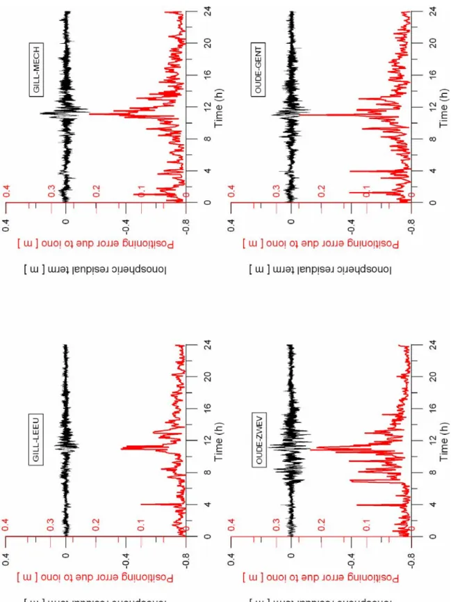
5.2.1 Quiet day 103/07 (figure 5.1)

For the whole quiet day in terms of ionospheric disturbances, we can see that the ionospheric residual term (plotted in black) is very close to zero for all of the analyzed baselines. The positioning error (red line) due to the ionosphere sometimes

ij GF AB

reaches the value of 4-5 cm, particularly for the 20 km long baselines GILL-MECH, OUDE-ZWEV and OUDE-GENT. We can observe that, on average, the positioning error is quite lower for the smallest baseline than for the other ones. Let’s recall that the nominal RTK accuracy level is a few centimeters. Therefore, we can consider that ionospheric effects of 4-5 cm are not “out of tolerance”, in particular for a 20 km baseline.

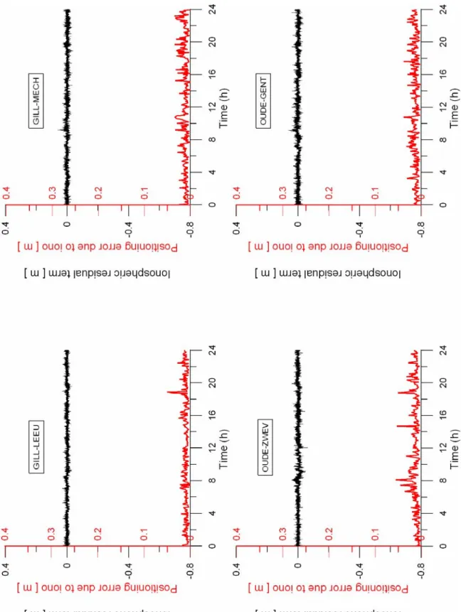
5.2.2 Day with medium-amplitude TID: 359/04 (figure 5.2)

From the residual term we can observe that the ionospheric activity induced by the TID occurred mainly between 8 A.M. and 2 P.M. with a maximal variability around 10 A.M. These observations are in agreement with the ionospheric variability observed with the one-station method (see figure 5.3 in WP 220). We can also observe that the positioning error increases when increases; this effect is observed for all baselines.

ij GF AB I _, ij GF AB I _,

The absolute value of the ionospheric residual term is generally lower for the smallest baseline GILL-LEEU than for the other ones. The maximal positioning error values reached for the baselines GILL-LEEU are about 9 cm while these values exceed 10-12 cm for a few cases on longer baselines. The largest positioning error has been observed for the baseline GILL-MECH and is close to 15 cm, what is significantly larger than the maximum value obtained in section 4 based on a 15 minute period only.

ij GF AB

I _,

Let us note that this largest value of 15 cm was not due to the TID observed around noon but was due to a small structure similar to a TID which occurred during 30 minutes around 18h30. Let us also remark that this structure was not visible for all the analyzed baselines: for example, the ionospheric residual term ij

GF AB

I _, remains very quiet for

OUDE-ZWEV while OUDE-MECH clearly detected the structure. This observation confirms the conclusions of WP 220: the baseline orientation has clearly an influence on the way that ionospheric structures are “seen” in double differences. Moreover, the positioning error due to ionosphere seems to be correlated with the term ij

GF AB

I _, because

the peak in positioning error appears simultaneously than this small ionospheric structure for OUDE-MECH.

5.2.3 Day with large-amplitude TID: 301/03 (figure 5.3)

The analysis of figure 5.3 shows that the TID induces an increase in the ionospheric residual term from 6-7 A.M. to approximately 2 P.M. The temporal variability of this term is smaller for the smallest baseline GILL-LEEU than for the other ones, as it is the case for the TID of DOY 359/04. This observation is in accordance with the results obtained in WP 220 (see section 5.5.2 WP 220) which conclude that the ionospheric residual term increases with increasing baseline length. Moreover, we can observe that,

ij GF AB

as for the TID of DOY 359/04, the positioning error is also smaller for this same baseline GILL-LEEU.

The maximal positioning error is observed for the baseline OUDE-GENT at 11 A.M. However, let us remind that a powerful solar flare occurred exactly at the same time; this flare increased dramatically the TEC and the variability in TEC (RoTEC) was very large during a few minutes (see WP 220 section 4.2.2). Therefore, we have not to take this period into account to assess the effect of the large-amplitude TID which appeared earlier and disappeared later than the solar flare, which induces a very sudden ionospheric phenomenon. If we have a look at the positioning error earlier or later than 11 A.M, we can see that the maximum values are larger than the maximum values relative to the medium-amplitude TID of DOY 359/04. If we do not take the positioning error of 11 A.M. into account, the maximal positioning error during the day has been observed for the baseline GILL-MECH; its value is about 22 cm. Nevertheless, we can also conclude that the largest positioning error on a 20 km baseline due to a powerful solar flare is approximately 25 cm.

5.2.4 Day with severe geomagnetic storm: 324/03 (figure 5.4)

Figure 5.4 shows that the ionospheric effects due to the geomagnetic storm took place from noon and lasted until the end of the day. However, we can identify two very variable periods around 17h and 22h. The ionospheric residual term and the positioning error due to the ionosphere are the largest during these two time intervals.

We can also observe from figure 5.4 that the ionospheric effects (in ij GF AB

I _, term and also

in the positioning error) are smaller for the smallest baseline GILL-LEEU, as for the previous disturbed days.

The daily maximum value of the positioning error due to the ionosphere has been observed for the baseline GILL-MECH and is about 80 cm.

Figure 5.1. Ionospheric effects on term (black) and on the positioning error (red) for DOY 103/07.

ij GF AB

Figure 5.2. Ionospheric effects on term (black) and on the positioning error (red) for DOY 359/04.

ij GF AB

Figure 5.3. Ionospheric effects on term (black) and on the positioning error (red) for DOY 301/03.

ij GF AB

Figure 5.4. Ionospheric effects on term (black) and on the positioning error (red) for DOY 324/03.

ij GF AB

5.3. Positioning error and ambiguity resolution

Positioning error values obtained in sections 4 & 5 correspond to the positioning error only due to the ionosphere and are representative only for RTK users who have already fixed their ambiguities to the correct integer values. Indeed, in our study, the ambiguities are solved using our own software which takes into account the whole visibility period of the different satellite pairs; the ionospheric effects are assessed afterwards. Therefore, this method is not representative of the error which will be experienced by a user during the so-called “initialization phase” where he has to wait that ambiguities are solved to the correct integer before starting surveying. In practice, positioning error obtained during the occurrence of ionospheric disturbances can reach values which are much larger than values obtained in sections 4 & 5 because such structures can affect the real-time ambiguity resolution process implemented in the user’s receiver. Indeed, if during the ambiguity resolution process, the ionospheric residual term is equal to or is larger than half a GPS-cycle, the ambiguities might be fixed to wrong integer values, which can lead to very large positioning errors. This effect has not been taken into account in our study. However, we implemented a method allowing a real-time ambiguity resolution process based on float ambiguities and their covariance matrix as input: the so-called “LAMBDA” method (Joosten & Tiberius, 2000). In order to illustrate the positioning error that a user can experience on the field in case of ionospheric disturbances, we chose to plot the positioning error during the occurrence of the medium-amplitude TID of DOY 359/04. As for our previous results, the positioning error is computed within 5 minute time intervals.

Figure 5.5. Positioning error for DOY 359/04 on baseline GILL-LEEU (11.3 km) when considering the LAMBDA ambiguity resolution technique.

The analysis of figure 5.5 shows that positioning error values exceed 1 m and can reach nearly 3 m for a baseline of only 11 km. When comparing these values with the values discussed in section 5.2.2, we can observe that the errors obtained with the real-time method are more than ten times larger than the values obtained if the ambiguities are correctly solved. In fact, if ambiguity resolution gives wrong integer values during the initialization phase, the user position will be affected by these wrong ambiguities during the whole surveying period. However, although the positioning errors obtained with the real-time method correspond to the real situation encountered on the field, they do not reflect the direct effects of the ionosphere on positioning when the ambiguities have been successfully solved. In reality, it is not very useful to assess ionospheric error during initialization phase: the magnitude of the error experienced during initialization is not an important parameter. It is much more realistic to assess the ionospheric error after ambiguity resolution: it allows to warn users when the level of ionospheric error reaches half a cycle, what will clearly be the origin of strong degradations for users who are trying to solve their ambiguities.

6 QUANTITATIVE STUDY OF THE POSITIONING ERROR DUE TO THE NEUTRAL ATMOSPHERE

In WP 250, we have developed an index which allows to detect the presence of small-scale structures in the neutral atmosphere. In this section, we use the technique outlined in section 3 to assess the influence of such structures on RTK positioning: we compute the absolute value of the difference between the “true” station position and the computed position (XB,2 , YB,2 , ZB,2) which is obtained based on double differences corrected for

differential ionospheric effects. It is important to underline that this strategy has a disadvantage: not only small-scale structures in the neutral atmosphere can be the origin of large differences between these positions; indeed, other error sources still affect the computed position (XB,2 , YB,2 , ZB,2):

- Residual multipath and measurement noise; - Bad satellite coverage (bad geometry);

- Tropospheric “thickness”: it is important to recall that our tropospheric index has been developed in order to detect irregular structures; it is computed based on double differences of the ionospheric-free combination. In practice, to isolate the effects of small-scale structures on this combination, we fit it using a 3rd order polynomial and we compute residuals to the fit. This procedure removes elevation effects (see WP 250 figure 15 p. 26), i.e. tropospheric differential effects due to satellites at low elevations. These effects which usually remain negligible for short baselines (< 10 km) can become larger for baselines of about 20 km. It is also important to recall that the goal of our project is to detect phenomena which could pose a threat for high accuracy real time positioning; therefore, “elevation effects” are outside of the scope of our study.

From equation 2.10 in WP 250, it can be seen that positions computed using ionospheric-free combination are affected by the same error sources as the positions computed by the method outlined in section 3. In addition, the measurement noise of the ionospheric-free combination is larger. This is the reason why we did not use the ionospheric-free combination to assess the positioning error due to small-scale structures in the neutral atmosphere. −0.7 −0.6 −0.5 −0.4 −0.3 −0.2 −0.1 0 0.1 0.2 0.3 0.4 0.5 0.6 0.7 2 3 4 5 6 7 8 9 Error on RTK − positioning solutions Day of January 2006

Reference station (BRUS) for the rover (BERT) North component East component Up component 0 0.1 0.2 0.3 0.4 0.5 0.6 0.7 2 3 4 5 6 7 8 9

Positioning error due to troposphere [m] _{Day of January 2006}

BRUS−BERT (19 km)

Figure 6.1 Error on RTK positions for north, east and up components (on the left) of baseline BRUS-BERT; positioning error expressed in distance is shown on the right.

0 1 2 3 4 5 6 7 8 9 10 11 12 13 14 15 16 17 18 19 20 2 3 4 5 6 7 8 9 IF DD Index (cm) Day of January 2006 BRUS−BERT Baseline (19 km)

Figure 6.2 IF DD Index for baseline BRUS-BERT from 02/01/2006 to 09/01/2006. To be able to “extract” the contribution of small-scale tropospheric structures to the positioning error obtained from the method outlined in section 3, it is important to assess the positioning error experienced during quiet tropospheric conditions (as measured by our tropospheric index).

In figure 6.1 we present the error on RTK positions for the three components of BERT station (rover) considering BRUS as reference station from 02/01/2006 to 09/01/2006. The error on the three components of the position can also be expressed in terms of distances according to equation (5.1). The 7 days selected in January 2006 present small IF DD Index (see table 1 of WP 250 and figure 6.2). Despite the fact that no IF DD Index larger than 4 is observed during these days, we can see that for a baseline of about 20 km, the positioning error (distance) due to all error sources (except ionosphere and small-scale structures in troposphere) ranges from a few centimetres up to about 18 cm. This level of error can be explained by the fact that 20 km is considered as the maximum acceptable baseline length for usual RTK applications.

0 0.1 0.2 0.3 0.4 0.5 0.6 0.7 12 13 14 15 16 17 18 19

Positioning error due to troposphere [m] _{Day of January 2006}

BREE−MEEU (7 km) −0.7 −0.6 −0.5 −0.4 −0.3 −0.2 −0.1 0 0.1 0.2 0.3 0.4 0.5 0.6 0.7 12 13 14 15 16 17 18 19 Error on RTK − positioning solutions Day of January 2006

Reference station (BREE) for the rover (MEEU) North component

East component Up component

Figure 6.3 Error on RTK positions for north, east and up components (left) and on distance for baseline BREE-MEEU from the 12/01/2006 to 19/01/2006.

0 1 2 3 4 5 6 7 8 9 10 11 12 13 14 15 16 17 18 19 20 12 13 14 15 16 17 18 19 IF DD Index (cm) Day of January 2006 BREE−MEEU Baseline (7 km)

Figure 6.4 IF DD Index of baseline BREE-MEEU from the 12/01/2006 to 19/01/2006. We performed the same test for baseline BREE-MEEU (7km) from 12/01/2006 to 19/01/2006; IF DD Index is smaller or equal to 3 during the whole considered period what represents quiet tropospheric conditions (figure 6.4). Figure 6.3 shows that the positioning error remains smaller than 10 cm except in a few cases (4 cases on 7 days). From this point, we can conclude that it will be much easier to “extract” the contribution of small-scale tropospheric structures to the positioning error by analyzing shorter baselines.

In practice, we processed the days with the largest IF DD Index values for the baselines which have been studied in WP 250: BRUS-BERT, BRUS-OLLN, BREE-MEEU. We present here the main conclusions from this study:

1) In most of studied cases, IF DD Indexes larger or equal to 5 (the so-called “5+” category in WP 250) are the origin of degradations in positioning errors which range between 20 cm and 40 cm even on short baselines (35 cm on BREE-MEEU (7 km) and 31 cm on BRUS-GILL (4 km) ). 0 0.1 0.2 0.3 0.4 0.5 0.6 0.7 0 1 2 3 4 5 6 7 8 9 10 11 12 13 14 15 16 17 18 19 20 21 22 23 24

Positioning error due to troposphere [m] _{DOY 209, year 2006, Time (h)}

BRUS−BERT (19 km) 0 1 2 3 4 5 6 7 8 9 10 11 12 13 14 15 16 17 18 19 20 0 1 2 3 4 5 6 7 8 9 10 11 12 13 14 15 16 17 18 19 20 21 22 23 24 IF DD Index (cm)

Year 2006, DOY 209, Time (h) BRUS−BERT Baseline (19 km)

Figure 6.5 Errors on distance (left) and IF DD Index (right) for baseline BRUS-BERT on 28/07/2006.

Figure 6.5 shows IF DD index and errors on distance for baseline BRUS-BERT observed on 28/07/2006 when heavy rainfalls have been observed (see WP 250 for more details). Even if the “background” positioning error on baseline BRUS-BERT ranges from 5 cm to 20 cm, the occurrence of IF DD Indexes of 5+ category is the origin of increased positioning errors of more than 30 cm.

0 0.1 0.2 0.3 0.4 0.5 0.6 0.7 0 1 2 3 4 5 6 7 8 9 10 11 12 13 14 15 16 17 18 19 20 21 22 23 24

Positioning error due to troposphere [m] _{DOY 209, year 2006, Time (h)}

GILL−BRUS (4 km) 0 1 2 3 4 5 6 7 8 9 10 11 12 13 14 15 16 17 18 19 20 0 1 2 3 4 5 6 7 8 9 10 11 12 13 14 15 16 17 18 19 20 21 22 23 24 IF DD Index (cm)

Year 2006, DOY 209, Time (h) BRUS−GILL Baseline (4 km)

Figure 6.6 Errors on distance (left) and IF DD Index (right) for baseline BRUS-GILL on 28/07/2006.

Figure 6.6 shows IF DD Index and errors on distance for baseline BRUS-GILL (4 km) observed on 28/07/2006. IF DD Indexes of 5+ category are observed from 12h00 to 17h00, which corresponds to positioning errors up to 30 cm, even on such a short baseline. It is clear that in the case of short baselines, it is easier to “extract” the contribution of small-scale tropospheric structures from the background positioning error.

0 0.1 0.2 0.3 0.4 0.5 0.6 0.7 0 1 2 3 4 5 6 7 8 9 10 11 12 13 14 15 16 17 18 19 20 21 22 23 24

Positioning error due to troposphere [m] _{DOY 180, year 2005, Time (h)}

BRUS−BERT (19 km) 0 1 2 3 4 5 6 7 8 9 10 11 12 13 14 15 16 17 18 19 20 0 1 2 3 4 5 6 7 8 9 10 11 12 13 14 15 16 17 18 19 20 21 22 23 24 IF DD Index (cm)

Year 2005, DOY 180, Time (h) BRUS−BERT Baseline (19 km)

Figure 6.7 Errors on distance (left) and IF DD Index (right) for baseline BRUS-BERT on 29/05/2005.

Figure 6.7 shows IF DD index and errors on distance for baseline BRUS-BERT (19 km) observed on 29/05/2005. This event has also been studied in details in WP 250. IF DD Indexes of 5+ category are observed from 00h00 to 01h00 and from about 11h30 to

15h30. In this case, the error due to small-scale tropospheric structures cannot be extracted from the background error.

2) There is no “linear” relationship between the magnitude of the IF DD Index and the magnitude of the positioning error. This fact can be understood rather easily: as already explained, the station position is computed based on a least square adjustment of all available satellite pairs for the considered period. On the one hand, the number of satellite pairs which are affected by the structures has an important influence on the positioning error: for example, conditions where 5 satellite pairs are affected by an index of 5 could be the origin of larger errors than conditions where only one satellite is affected by a large index of 15. On the other hand, from the theory of error propagation, we know that an increased uncertainty on the measured quantities (double differences) results in an increased uncertainty in the derived parameters (positions): this means that a larger error in the double differences gives a higher probability to have a larger error in the computed position but this position will not necessarily be larger in the reality.

This is illustrated by figure 6.8 which shows IF DD Index and errors on distance for baseline BREE-MEEU observed on 06/06/1998: between 07h00 and 8h00, an index of 6 is observed while the positioning error is close to 30 cm; around 17h00, an index of 13 is observed while the positioning error is close to 10 cm (rather close to the background error). 0 0.1 0.2 0.3 0.4 0.5 0.6 0.7 0 1 2 3 4 5 6 7 8 9 10 11 12 13 14 15 16 17 18 19 20 21 22 23 24

Positioning error due to troposphere [m] _{DOY 157, year 1998, Time (h)}

BREE−MEEU (7 km) 0 1 2 3 4 5 6 7 8 9 10 11 12 13 14 15 16 17 18 19 20 0 1 2 3 4 5 6 7 8 9 10 11 12 13 14 15 16 17 18 19 20 21 22 23 24 IF DD Index (cm)

Year 1998, DOY 157, Time (h) BREE−MEEU Baseline (7 km)

Figure 6.8 Errors on distance (left ) and IF DD Index (right) for baseline BREE-MEEU on 06/06/1998.

3) We sometimes observe still unexplained peaks in the positioning error time series. Some of them are larger than one meter and have been considered as outliers: they are probably related to unfixed problems in our software. In other cases, we observe smaller peaks (see for example the peak in figure 6.6 between 2h00 and 3h00 which does not correspond to a period with large IF DD Index). It could be due to other problems like bad geometry, for example. Further investigations are necessary to understand the origin of these peaks.

7 IONOSPHERIC EFFECTS ON AVIATION

Applications in aviation are based on carrier-smoothed code observables. Aircrafts use differential corrections provided by reference stations in order to improve the accuracy of their computed positions.

For a given satellite i, the code measurement made by the user (aircraft) is affected by an ionospheric error i

u

I (also called slant ionospheric delay) given by (equation 2.2):

2 40.3 i i u u TEC I f = (7.1) At the same time, the code measurement made by the reference station on the same satellite i is affected by an ionospheric error i

r I given by: 2 40.3 i i r r TEC I f = (7.2) The reference station provides i

r

I as ionospheric correction to the user. Therefore, the quality of the differential ionospheric correction will depend on de difference i

u i r

I − (the I difference in slant delays experienced by the user and by the reference station). This difference depends on TEC_{u r} (equations (7.1) and (7.2)). Small-scale structures in the ionosphere can be the origin of differences in slant delays which can pose a threat for applications in aviation.

i

ECi T −

Ionospheric storms can have significant adverse effects on the performance of present-day technological systems, including satellite navigation for aviation. Although the satellite-based navigation for aviation purposes possesses large capabilities and advantages above conventional navigation aids, the ionospheric effects in various applications/services are still poorly investigated /understood. The observation of ionospheric effects and their interpretation are complicated by the fact that the ionosphere dynamics and the ionospheric disturbances in particular are characterized by strong variations in the vertical and horizontal electron density distribution that depend also on season and local time.

The use of satellite navigation for precision vertical guidance requires precise correction and bounding of ionospheric delay estimation errors. WAAS (Wide Area Augmentation System) has already experienced major geomagnetic storms where vertical guidance has been automatically disabled for periods lasting several hours over most of the United States (Luo et al., 2003). The LAAS (Local Area Augmentation System) system assumption of a constant ionosphere variation in the area of the airport and detection of noncompliant conditions has been put under investigation since it is of high priority to the LAAS program. For the purpose, researchers have already observed and attempted to quantify the irregularity of the ionosphere during strong geomagnetic storms over CONUS in the last few years. Observations of significant ionospheric anomalies, including gradients, ‘depletion/irregularity walls’, and similar fast moving ionospheric features in the American sector have been reported for the major ionospheric storms on 6

April 2000, 29 October 2003, and 20 November 2003. For example, initial research into the rapid changes in delay during the geomagnetic storm of April 6th, 2000 identified the possibility that the delay changes were due either to very steep gradients of narrow “walls” (i.e. 20 km wide) moving slowly (100 m/s) or that these were somewhat wider walls (80—100 km) moving much more rapidly (~500 m/s) (Luo et al., 2003; Dehel et al., 2004). Closely spaced CORS observations of ionospheric delay changes are shown in Fig.7-1.

Fig.7-1. Ionospheric delay drop during the geomagnetic storm on 6 April 2000 at

multiple sites in the Washington D.C. area showing the ‘wall’ motion.

Observations of these ionospheric features remain limited and the underlying physics is still not well understood. Therefore, it will be interesting to learn if such features were observed in other longitudes during these or other strong geomagnetic storms, since the international GBAS (Ground Based Augmentation System) and SBAS (Space Based Augmentation System) systems will need to be provably-safe during geomagnetic storms (Dehel et al., 2004).

The research reported in this section addresses the issue of the ionospheric ‘irregularity walls’ and associated phenomena. Presented are our observations and research based on analyses of the local TEC / slant delay behaviour. Comparisons are made with the corresponding American observations during the storms of 29 October 2003 and 20 November 2003.

7.1 Case studies of ionospheric gradient anomalies

For the purpose of studying ionospheric gradient anomalies, we have selected several GPS stations in Belgium (Fig.7-2), namely BRUS (50°47'N, 04°21'E), DENT (50°56'N, 03°23'E), BREE (51°08'N, 05°38'E), WARE (50°41'N, 05°14'E), and DOUR (50°05'N, 04°35'E). Each station is assigned a unique colour code which will be used when plotting the measurements made at this station. The above-mentioned stations were selected because of their geographic locations, optimal distance from one another and alignment, suitable for detection of the ionospheric disturbances/anomalies we are focused on in this report.

Fig.7-2. Map of Belgium with the GPS stations used for this study.

Although data from all GPS stations was used, mostly results from the BREE-WARE-DOUR set of stations will be presented here. One important reason for such selection is the typical propagation patterns of ionospheric disturbances during storms. To demonstrate the propagation, the TEC relative deviation from median, DTEC=(TEC−TECmed)/TECmed , is used. The ratio enhances the perturbation effects and

facilitates the interpretation. For example, the observed increase of relative TEC between 0600 and 1400 UT during the storm on 24 July 2004 appears first at northern high latitudes and then propagates steadily in SW direction (Fig.7-3). The development and propagation of such an increase is explained with the action of an eastward directed electric field which penetrates from high latitudes toward lower latitudes and thus lifts up the plasma via the electromagnetic (E×B) drift effect, resulting in a reduced loss rate, that is, in a positive DTEC response.

Fig.7-3. Relative TEC observed during the storm on 24 July 2004 (Stankov et al., 2006). In fact, the ‘irregularity walls’, detected in the American sector during the storms of 6 April 2000, 29 October 2003, and 20 November 2003, all follow a similar propagation pattern.

7.1.1 The ionospheric storm on 29 October 2003

During the whole month of October 2003 the geomagnetic activity was low except during the last 3 days when a large storm took place. The events at the end of October 2003 were characterized by a series of large radiation bursts at the Sun and huge coronal mass ejections (CMEs) causing severe perturbations in the geomagnetic field and in the geo-plasma environment formed by the magneto- and ionosphere. On 28 October, while the sunspot group 486 faced directly toward Earth, a huge solar flare was observed which was the third largest on record since 1976. The corresponding CME left the sun at about 2000 km/s reaching the Earth magnetosphere already after 19 hours, around 06:00UT on 29-th October. The subsequent geomagnetic storm was one of the largest in the past 40 years continuing well into 30-th and 31-st of October. For most of the time on 29 October the recorded planetary geomagnetic index Kp was close to its maximum possible value of 9, indicating severe geomagnetic and ionospheric conditions (Fig.7-4). Similarly, the other geomagnetic index, Dst, strongly related to the magnetospheric parameters, reached values of about -400nT, thus confirming the extreme intensity and duration of the magnetic storm. These conditions set the background for observing and experiencing strong ionospheric effects.

Fig.7-4. The 29-31 October 2003 ionospheric storm background as represented by the

planetary geomagnetic indices Kp (top panel) and Dst (bottom panel)..

During the storm period of 29-31 October 2003, reported were several significant malfunctions due to the adverse effects of the ionosphere perturbations such as interruption of the WAAS service and degradation of mid-latitudes GPS reference services. Analyses of this storm also revealed steep “walls of depletion” (Fig.7-5) moving through with high speeds and gradients of hundreds of mm/km (Dehel et al., 2004).

Fig.7-5. Large ionospheric delay gradients (‘walls’) (left panel) observed among CORS

clusters in the Washington D.C. area (right panel) on 29 October 2003.

As already stated, it will be interesting to see if similar anomalies are observed here in Europe. For the purpose, we have analysed all available observations carried out at the selected network of GPS stations in Belgium during this particular ionospheric storm. The ionospheric delay measurements from 29 October 2003 deduced from all satellite links are plotted in the upper panel of Fig.7-6 with references to the corresponding ionospheric piercing points (IPP) given in the bottom panel. The figure clearly shows the sharp increase of the ionospheric delay during the main phase of the storm in the morning hours. This increase is sustained well into the afternoon hours in accordance to the extreme geomagnetic activity conditions (cf. Fig.7-4). It is followed by a significant drop of the delay values in the period between 1700 and 2000 UT. Hence, it is more likely to observe ‘depletion wall’ in this time period.

Fig.7-6. Ionospheric delays during the storm on 29 October 2003 measured via the GPS

satellites ‘visible’ from the selected GPS stations in Belgium (top panel). The satellite IPP traces over Europe (with reference to the base reference station BRUS) are plotted in the bottom panel with red colour. The period of ‘visibility’ of each GPS satellite, again with reference to the BRUS station and according to UT, is plotted in the bottom panel with black solid lines.

The figure also suggests that a proper detection and analysis of ‘depletion walls’ will have to deal with various inconveniences, such as the irregular coverage of the satellite IPP traces, different shape and orientation of these traces, short-term visibility of GPS satellites, etc.