Effect of undisturbed ground temperature on the design of closed-loop geothermal systems: a case study in a semi-urban environment
G. Radiotia*, K. Sartorb, R. Charliera, P. Dewallefb and F. Nguyena a
ArGEnCo department, University of Liege, Allée de la Découverte 9, 4000 Liege, Belgium b
A&M department, University of Liege, Allée de la Découverte 17, 4000 Liege, Belgium *Corresponding author: gradioti@ulg.ac.be
Abstract
This paper presents temperature measurements in four Borehole Heat Exchangers (BHEs), equipped with fiber optics and located in a semi-urban environment (campus of the University of Liege, Belgium). A 3D numerical model is also presented to simulate the heat loss from the surrounding structures into the subsurface. The mean undisturbed ground temperature was estimated from data during the preliminary phase of a thermal response test (water circulation in the pipe loops), as well as from borehole logging measurements. The measurements during water circulation can significantly overestimate the ground temperature (up to 1.7 °C in this case study) for high ambient air temperature during the test, resulting in an overestimation of the maximum extracted power and of the heat pump coefficient of performance (COP). To limit the error in the COP and the extracted power to less than 5%, the error in the undisturbed temperature estimation should not exceed ±1.5 °C and ±0.6 °C respectively. In urbanised areas, configurations of short BHEs (length < 40 m) could be economically advantageous (decreased installation and operation costs) compared to long BHEs, especially for temperature gradient lower than -0.05 °C/m.
Keywords
undisturbed ground temperature, TRT rig insulation, numerical modelling, urbanisation effect, design Nomenclature A cρ D ṁ q Q Qref Qw T Tair Tavg,ground TC Tfix Tg Tm TH Tref Tw Tw,entrance Tw,exit V
annual oscillation amplitude of temperature (°C) specific heat capacity (J/kgK)
depth (m)
mass flow rate (kg/s) heat transfer rate (W)
maximum extracted power (W/m) maximum extracted power for Tref (W/m) maximum extracted power for Tw (W/m) temperature (°C)
air temperature (°C)
depth-average ground temperature (°C) temperature of the cold reservoir (K) fixed temperature (°C)
undisturbed ground temperature (°C) average annual air temperature (°C) temperature of the hot reservoir (K)
reference ground temperature (fiber optics) (°C) water temperature (°C)
water temperature at the entrance of the rig (°C) water temperature at the exit of the rig (°C) volumetric flow rate (l/min)
Greek symbols
αg η
ground thermal diffusivity (m²/d) heat pump efficiency (-)
Abbreviations BHE COP DTS RTD SEGI TRT
Borehole Heat Exchanger Coefficient of Performance Distributed Temperature Sensing Resistance Temperature Detector General Service of Informatics Thermal Response Test
3 1. Introduction
Geothermal heat pumps are widely used for heating and cooling, with an increasing number of applications over the last years [1, 2]. Shallow geothermal heat pump systems (<400 m depth) exchange heat with the ground either by circulating the groundwater through two separate wells (open-loop) or by circulating a fluid in closed pipe loops embedded in the ground mass (closed-loop) [3, 4]. Vertical closed-loop geothermal systems, also known as Borehole Heat Exchangers (BHEs), are widely used since they have a small footprint at the ground surface, can be applied in many hydrogeological contexts, are more efficient than horizontal systems and provide lower environmental impact compared to open-loop systems, which typically require a more constraining permit for installation. BHEs also provide economical and environmental benefits, compared to other heating systems (e.g. air source heat pumps, electric heaters, oil or natural gas boilers) [5-7]. However, they typically have higher installation cost which can result in long payback periods (typically until 20 years). Minimizing the installation and operation costs requires that the local geological and climate conditions are adequately considered [8-10].
The undisturbed ground temperature, i.e. the ground temperature before any heat injection or extraction, is a critical parameter for the design and the thermal performance of BHEs. It is well known that the ground temperature affects the coefficient of performance (COP) of the heat pump, limits the amount of power extracted from the ground and affects the required BHE length [11-13]. According to the numerical study of Dehkordi and Schincariol [14], a variation in the average ground temperature of 25% modifies the heat extraction rate by approximately 25%. Kurevija et al. [15] studied the effect of a high geothermal gradient (0.055 °C/m) on the design of BHEs, for a case study in Zagreb, Croatia. They concluded that estimating the mean ground temperature by including the influence of the geothermal
4 gradient can result in a decrease of the required pipe loop length, in the order of 4% - 7% for the different investigated borehole array grids. Therefore, an accurate estimation of the undisturbed ground temperature is crucial in order to optimise the design and to assure the long-term efficiency of BHEs.
The undisturbed ground temperature is determined in-situ by mainly two methods [16]. The first method consists in temperature logging along the borehole, usually by lowering a temperature probe into the U-pipe and measuring the temperature at several depth intervals or by installed temperature sensors or fiber optic cables along the [17, 18]. The second method consists in circulating the fluid inside the pipe loops without heat injection and recording the temperature at the pipe inlet and outlet. Both methods assume that a thermal equilibrium has been reached between the fluid inside the pipes and the ground and they estimate the mean ground temperature over the depth of the BHE by averaging the measured data. The second method is widely applied, since it consists in the preliminary phase of a Thermal Response Test (TRT). It has a typical duration of 2 h - 12 h [18]. The accuracy of this method depends on the accuracy of the measurement equipment and on the heat added to the circulating fluid due to friction and the pump work. The latter can result in a significantly overestimated undisturbed temperature, especially in the case of relatively large circulation pumps (e.g. overestimation of 2 °C after 60 min of circulation [19]). Another important factor is the insufficient TRT equipment insulation, since it can result in oscillations in the recorded temperature evolution. Studies mainly focus on the influence of the insulation on the accuracy of the estimated thermal conductivity and borehole thermal resistance [20-22]. However, its effect on the undisturbed ground temperature estimation should also be investigated, since this parameter is critical for the design of BHEs.
5 Concerning the undisturbed ground temperature distribution, three zones can be typically distinguished [23]. In the surface zone (until ~1 m depth), ground temperature is strongly affected by the weather conditions. In the shallow zone, varying from 1 m to 20 m depth depending on the local ground type, temperature is mainly influenced by the seasonal weather conditions. At the end of this zone, ground temperature is close to the average annual air temperature. The deep zone follows, where temperature is invariant with time and increases with depth according to the local geothermal gradient. Deviations from this distribution can be observed in the case of groundwater flow, varying ground thermal properties and/or anthropogenic effects. The latter results in elevated ground temperatures with zero or negative temperature gradients extending to depths more than 50 m, which is observed worldwide in urban areas [24-27]. In-situ case studies of temperature borehole logging have revealed increased ground temperatures, which are attributed to the urbanisation effect mainly based on observations of building presence and occupation close to the measurement locations [28-30].
The analytical studies of Rivera et al. [31, 32] highlight the effect of land surface conditions (e.g. asphalt layers, new buildings) on the temperature field evolution around BHEs and their influence on the geothermal potential in urbanised areas. According to their study [33], elevated ground temperatures in urban areas can increase the extractable energy up to 40% compared to rural areas. This can result in a decrease of the borehole length of 4 m for each additional degree of ground heating. Their findings highlight the geothermal potential in urbanised areas, where the heat loss through structures recharges the geothermal reservoir. However the effect on the heat pump COP is not addressed, which determines the operational cost of the BHE system. Moreover, in order to minimize the installation cost in urbanised
6 areas, there is a need for an easy-to-implement and cost-effective approach that considers the local ground temperature conditions and can be applied in each individual BHE installation.
This paper focuses on the effect of the undisturbed ground temperature on the design of BHEs based on experimental and numerical results. It presents temperature measurements in four BHEs of 100 m long equipped with fiber optics located on the campus of the University of Liege, Belgium, in close distance to a building and an underground heating structure (feeder pipe). We investigate the accuracy of the undisturbed temperature estimation from TRT data, in the case of insufficient test rig insulation, and we evaluate its effect on the design of BHEs. Moreover, in this paper it is argued that the measured ground temperature profiles, before the in-situ TRTs, are the result of structures heat loss into the subsurface. We present a 3D numerical model to further investigate this argument and we estimate the temperature field evolution in the surrounding ground. We compared short with long BHE configurations for applications in urbanised environments by evaluating the heat pump COP and the total required BHE length. We propose a cost effective, widely applicable approach that could minimize the installation and operation costs in urbanised areas.
The remainder of the paper is organised as follows. First the site description is presented together with the materials and methods used in this study. Then the fiber optic measurements in the four BHEs in a period of 2 years are presented and discussed. The measurements during water circulation (TRT) follow, as well as their correlation to the ambient air temperature. The accuracy of the undisturbed temperature estimation and its effect on the design follow. Then, analytical and numerical results are presented and compared to the in-situ measurements. The effect of the heat loss through structures into the subsurface on the design of BHEs (COP, BHE length) is studied. Finally, we provide
7 conclusions and comments on the importance of a sufficient test rig insulation and on the urbanization effect with regard to the optimisation of BHEs.
2. Site set-up
2.1 Site location and geological settings
The site consists of four double-U BHEs (namely B1-B4) installed in the summer of 2013 on the campus of the University of Liege (Liege, Belgium). During the pipes installation, fiber optic cables were attached along the pipe loops [34, 35]. The cables were tapped every 50 cm at the outer surface of the pipes. Additionally to the fiber optic cables and in direct contact with them, two Resistance Temperature Detector (RTD) probes (Class A, ±0.15 °C) were attached at certain depths in each borehole. The BHEs were installed over a surface of 32 m² close to buildings and to the university feeder pipe, which is part of the campus district heating network (Figure 1). The building of the General Service of Informatics (SEGI), constructed in 1980, has a minimum distance of 15 m from the boreholes. The feeder pipe, buried in the ground at an average depth of 2.5 m, is operating since 1970 and has a minimum distance of 6.6 m from the boreholes. It consists of 6 pipes, each covered by a mineral wool insulation layer of a thickness of 12 cm, enclosed in a concrete shell of a thickness of 18 cm.
8 Figure 1 - Site location on the campus of the University of Liege (retrieved from Google Earth©) (red
line: heating feeder pipe, SEGI: General Service of Informatics, B1 to B4: four BHEs)
The site geology is characterised by deposits of sand and gravel down to a depth of approximately 8 m. The bedrock follows which is quite heterogeneous and consists mainly of siltstone and shale interbedded with sandstone. The average layer dip angle is approximately 45° SE and fractured zones are detected in the rock mass mainly down to a depth of 35 m. A detailed bedrock characterisation based on borehole televiewer measurements, cuttings thermal conductivity measurements and temperature profiles obtained in the four boreholes is presented in Radioti et al. [36]. The mean ground thermal conductivity is 2.88±0.16 W/mK, based on TRTs conducted in situ in the four BHEs [37].
9 2.2 Materials and methods
2.2.1 Temperature measurements
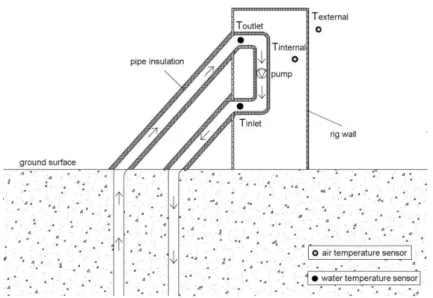
To conduct the in situ tests, the BHEs pipes were connected to a rig which encloses the typical TRT equipment [38]: a pump, an electric resistance heater, temperature sensors and a data logger. Insulation layers of 2 cm thick were attached around the connecting pipes, to minimize air temperature effects, while the rig wall (plastic honeycomb plate) was not insulated. Water and air temperature was recorded with an accuracy of ±0.15 °C (Class A) and ±0.30 °C (Class B) respectively (Figure 2). Temperature, flow rate and electrical power were recorded at a time interval of one minute.
Figure 2 - Temperature sensors location during water circulation in the pipe loops
Temperature was measured by the fiber optics before and during water circulation in the pipe loops in the four BHEs. Fiber optics allow to obtain continuous, high-resolution temperature profiles along the borehole lengths. Temperature is measured along the fiber optics, by applying the Distributed Temperature Sensing (DTS) technique [39]. This technique is based on Raman optical time domain reflectometry. The fiber optics are connected to the DTS instrument (Figure 3, left). A laser pulse is injected into the optical fiber and the light is scattered and reemitted from the observed point. The light is reemitted at wavelengths of
10 different frequency than the incident light (Raman scattering). Raman Stokes backscatter signals are characterised by frequencies lower than the one of the incident light, while anti-Stokes signals by frequencies higher than the one of the incident light (Figure 3, right). The Raman backscatter signal is temperature sensitive and the temperature along the fiber is determined by the intensity ratio of Raman Stokes and anti-Stokes signals. The position of the temperature reading is determined by the arrival time of the reemitted light pulse.
Figure 3 - Fiber optics connected to the DTS instrument (left) and sketch of Stokes and anti-Stokes Raman scattering (right)
Temperature was recorded every 20 cm (sampling interval) with a spatial resolution of 2 m in all the fiber optic measurements presented in this study. The temperature resolution (standard deviation) is of the order of 0.05 °C. The calibration of each in-situ obtained fiber optic profile was necessary, given that the calibration parameters vary with the operating conditions of the DTS instrument and the optical fiber itself [40]. The offset calibration was achieved by the temperature measurements of the attached RTD probes. In the case that the pipes were accessible (i.e. before connecting the TRT equipment), a RTD probe was also lowered into the pipe loop and temperature was measured at a depth interval of 10 m. This
11 allowed to investigate if these measurements can fairly reproduce the fiber optic profiles and to verify the attached RTD probes measurements.
Several measurements were conducted before the tests in a period of 2 years to detect any possible variation of the temperature profiles through time, with the first measurement conducted three weeks after the grouting injection. Temperature was also measured by the fiber optics during water circulation in the pipe loops, by applying a measurement time of 10 min or 60 min. Hence the obtained fiber optics profiles during the tests correspond to average temperature profiles of a time interval of 10 min or 60 min.
2.2.2 Analysis methodology
The fiber optic measurements were further studied by analytical and numerical modelling, to investigate if the measured temperature profiles could be attributed to the heating of the subsurface through the SEGI basement and the feeder pipe shell.
The undisturbed ground temperature for the Sart-Tilman area, Tg, was calculated by the heat diffusion analytical equation in a semi-infinite plane due to a temperature sinusoidal stress by including the geothermal gradient effect as [41]:
min 2 365 ( , ) exp cos ( ) 365 365 2 g m T geo g g D T D t T A D t t D ,
where D: the depth (m),
t: number of days from the first day of January (-),
Tm, the average annual temperature of the environment (Tm=8.9 °C),
12
tTmin, the day number corresponding to the minimum temperature (tTmin=10, from 1st January),
αg, the equivalent ground daily thermal diffusivity (αg=0.1104 m²/d) and
Tgeo(D): the product of the geothermal gradient, 0.013 °C/m for the Liege area [42], by the
testing depth.
The air temperature parameters used in this calculation are based on statistical data for the Sart-Tilman area for a period of 20 years [43] and the mean ground thermal conductivity on TRTs conducted in situ in the four BHEs (2.88 W/mK).
The 3D numerical model was developed by using the finite element code LAGAMINE [44, 45]. It includes the influence of the feeder pipe and of the SEGI building. The feeder pipe, which has a minimum distance of 6.6 m from the boreholes, was simulated with a surface heating element. The heat loss (150 W/m length) was calculated based on temperature measurements inside the feeder pipes for the year 2011 [46]. The SEGI is located close to the boreholes at a minimum distance of 15 m. The heat loss through the foundations of the SEGI building was simulated by imposing a constant temperature through time (17.7 °C) at the whole building surface, as measured by temperature data loggers at the basement of the building.
The ground was simulated with 4-node 3D finite elements down to a depth of 220 m, covering a surface area of 0.11 km² (80520 nodes). The applied ground thermal conductivity was estimated based on TRTs conducted in situ in the four BHEs (2.88 W/mK) and the volumetric heat capacity was taken equal to 2300 kJ/m³ K, based on literature values for the in-situ rock types [47, 48]. The initial ground temperature (i.e. before the presence of
13 structures) was estimated analytically, as presented above, without taking into account the influence of the variation of the air temperature. In this model, the simplified assumption was made that at bare ground the temperature is constant through time, equal to the average annual air temperature. Moreover, the ground surface under the pavements was simulated by a no-heat-flux boundary condition, since pavements usually display a much lower thermal diffusivity than the ground of this case study. The computational time was 1.5 h (computer with main memory 16 G RAM, processor Intel I7) for an investigated period of 60 years (1970-2030).
The urbanisation effect on the design of BHEs was studied by investigating the influence of the ground temperature profile on the maximum extracted power, the required borehole length and the heat pump COP. The maximum extracted power (W/m length of the BHE) was estimated based on the MCS 022 (MIS 3005 [13]) look-up tables for 1200 annual full load equivalent run hours of heat extraction, borehole thermal resistance of 0.1 mK/W, single U-pipe configuration and borehole spacing of at least 6 m. The heat pump coefficient of performance was calculated as:
H c H C T COP COP T T ,
where η: the system efficiency (η=0.5),
COPC: the theoretical maximum efficiency (-),
TH: the temperature at the hot reservoir (TH=313.15 K) and
TC: the temperature at the cold reservoir, i.e. ground (K).
The above formula is simple yet accurate enough to assess the influence of source temperatures on the efficiency of heat pumps for domestic and tertiary building heating.
14 3 Results
3.1 Undisturbed ground temperature estimation 3.1.1 Borehole logging before the in-situ tests
Figure 4 shows undisturbed temperature profiles measured in B2 in a period of two years. The upper 18 m correspond to the thermally unstable zone, where ground temperature is influenced by weather conditions. Below this depth, measured temperatures appear invariant to time in the two-year period. The temperature decreases through depth at a mean rate of approximately 0.25 °C/10 m and the depth-average temperature of this zone is 11.0 °C. In terms of spatial impact, B2, B3 and B4 display the same temperature distribution with depth (Figure 5). However in B1 a lower temperature than the other 3 boreholes was recorded in the first 20 m. RTD probe measurements, obtained with a depth interval of 10 m, can fairly reproduce the corresponding fiber optics profiles.
15 Figure 5 - Undisturbed ground temperature measured by the fiber optics and by lowering a RTD
probe inside the U-pipe in the four boreholes
Temperature was also measured by a RTD probe in a borehole well, which is located 150 m southeast from the site (Figure 6). The well is filled with water below a depth of 10.6 m. The influence of the air temperature (3.26 °C) is evident in the first meters. Below approximately 14 m, temperature oscillates around a value of 10.1 °C, lower than the corresponding temperature in the four boreholes. Moreover, contrary to what is observed in the four boreholes, the temperature is not decreasing through depth. The temperature profiles measured in the four BHEs and in the well are further studied by analytical and numerical modelling in section 3.2.
16 Figure 6 - Undisturbed ground temperature measured by lowering a RTD probe inside the borehole
well (24 February 2016)
3.1.2 Temperature during water circulation in the pipe loops 3.1.2.1 Inlet and outlet water temperature
Figure 7 shows temperature measurements during water circulation in the pipe loops in B1 and B2, conducted in summer (June 2014 and June 2015 respectively). In a perfect insulated system, the circulating water temperature would be invariant to the outside air temperature variations. The inlet and outlet pipe water temperature would quickly adapt to the depth-average ground temperature and would remain constant with time, in the case that no significant heat is added to the water due to the pump work. Based on the measured data, the air temperature inside the rig follows the outside air temperature variations and is an evidence for the heat transfer through the rig wall. This correlation is also displayed by the water measurements at the pipe inlet, while the pipe-outlet measurements seem less influenced by the air temperature variations. Moreover the temperature at the pipe inlet (rig exit) is higher than the one at the pipe outlet (rig entrance) during the whole test duration, which indicates
17 that heat is added to the water during its circulation inside the rig. The opposite effect is displayed in Figure 8, which shows temperature measurements for lower ambient air temperature. In this case, water temperature decreases during its circulation inside the rig, for most of the test duration, which indicates that heat is transferred from the water to the air.
Figure 7 - Air (top) and water (bottom) temperature measurements during water circulation in B1(June 2014) and in B2 (June 2015)
18 Figure 8 - Air (top) and water (bottom) temperature measurements during water circulation in B3
(March 2014) and in B4 (Nov. 2013)
The rate of the heat transfer from/to the water during its circulation inside the rig can be calculated from the convective heat transfer equation as:
, ,
( )
p w exit w entrance
qmc T T ,
where ṁ: the mass flow rate (kg/s),
cp: the specific heat capacity of water (cp=4.19 kJ/kgK at 10 °C),
Tw,entrance: the water temperature at the entrance of the rig (pipe outlet) (K) and
Tw,exit: the water temperature at the exit of the rig (pipe inlet) (K).
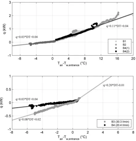
The calculated heat transfer rate is the result of the interaction with the air inside the module, as well as of the heat added to the water due to the pump work. Figure 9 shows the correlation of the heat transfer rate with the temperature difference T Tair Tw ent rance, for
19 small values of the constant b (-0.02 kW to 0.07 kW). In the case of positive temperature difference, heat is added to the water due to the interaction with the air, as well as due to the pump work. The interpolation lines are in good agreement with each other with a mean value of q0.11 T 0.06, for approximately the same applied flow rate (20 l/min to 22 l/min). Though extrapolation of this line for negative temperature difference is not representative of the measured data. In this case, heat is extracted from the water due to the interaction with the air, while heat is added to it due to the pump work. This could be the reason for the lower inclination of the interpolation line observed in the case of negative temperature difference. Increasing the flow rate induces an enhanced convection, which is illustrated by an increase in the a coefficient of the interpolation line (Figure 9, bottom).
Figure 9 - Heat transfer rate during water circulation inside the rig, as a function of the temperature difference between the water entrance temperature and the air temperature inside the rig, for
20 3.1.2.2 Estimation error and impact on the design
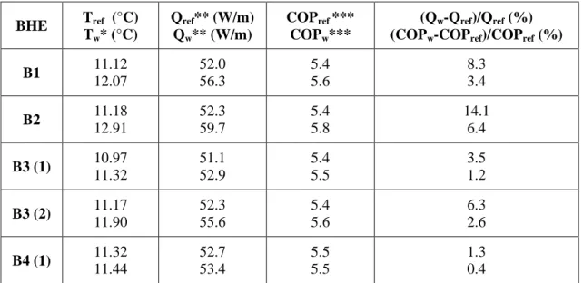
Despite the pipe insulation, the water measurements can be significantly influenced by the temperature air variations, which can result to an over or underestimation of the ground temperature. Table 1 shows the maximum overestimation of the ground temperature based on the water measurements and the impact on the design. Reference values correspond to fiber optics measurements conducted at the beginning of the test, since the calibrated fiber optic profiles are not biased by ambient air temperature conditions. The maximum temperature overestimation (1.7 °C) is observed in the case of B2 and corresponds to air temperature 18 °C higher than the ground temperature. This results in an error in the maximum extracted power of 14% and in the heat pump COP of 6%, significantly higher than the one expected due to the measurements equipment accuracy (<1.5% for T±0.15 °C). To limit the error in the COP and the extracted power to less than 5%, the error in the undisturbed temperature estimation should not exceed ±1.5 °C and ±0.6 °C respectively.
These results indicate that insulating only the pipes is not sufficient for an accurate estimation of the ground temperature and highlight the importance of the test rig insulation to the test procedure. They also indicate that a single-value evaluation (e.g. at the end of the circulating phase) can result in a significant error, since it can be biased by a high ambient air temperature, resulting in undersizing the system and in malfunctions during its operation.
Table 2 and 3 present estimated undisturbed temperature based on time-average water temperature values at the pipe inlet and outlet respectively. For this case study, where air temperature varies significantly during the tests, the error is lower than the single-value evaluation for all the in-situ tests. The maximum temperature overestimation (0.7 °C) is observed, as before, in B2 but results in a lower overestimation of the extracted power (6.1%
21 instead of 14%) and of the COP (2.5% instead of 6.4%), considering the pipe inlet measurements. The pipe outlet temperature, less influenced by the air temperature variations than the pipe inlet temperature, reduces the error in the extracted power and in the COP to the half for continuously high air temperature during the test (B1, B2 and B3(2)). For the tests B3(1) and B4(1) the water measurements result in an overestimation of the ground temperature (<0.2 °C), despite the fact that air temperature is lower than the ground temperature for most of the test duration. This small overestimation can be attributed to the accuracy of the measurement equipment (section 2.2.1). Moreover, for low air temperature the final heat extracted by the fluid will be reduced due to the pump work added heat. This indicates that a smaller error is expected for low air temperature than for a corresponding high temperature.
Table 1 - Maximum overestimation of ground temperature based on water temperature measurements, maximum extracted power and coefficient of performance of the heat pump
BHE Tref (°C) Tw* (°C) Qref** (W/m) Qw** (W/m) COPref *** COPw*** (Qw-Qref)/Qref (%) (COPw-COPref)/COPref (%) B1 11.12 12.07 52.0 56.3 5.4 5.6 8.3 3.4 B2 11.18 12.91 52.3 59.7 5.4 5.8 14.1 6.4 B3 (1) 10.97 11.32 51.1 52.9 5.4 5.5 3.5 1.2 B3 (2) 11.17 11.90 52.3 55.6 5.4 5.6 6.3 2.6 B4 (1) 11.32 11.44 52.7 53.4 5.5 5.5 1.3 0.4 *Maximum water temperature after the first 5 min of circulation
**MCS 022 (MIS 3005 [13]), 1200 FLEQ run hours *** n=0.5, TH=40 °C
22 Table 2 - Time-average water temperature at the pipe inlet, maximum extracted power and coefficient
of performance of the heat pump
BHE Tref (°C) Tw (°C) Qref* (W/m) Qw* (W/m) COPref ** COPw** (Qw-Qref)/Qref (%) (COPw-COPref)/COPref (%) B1 11.12 11.81 52.0 55.1 5.4 5.6 6.0 2.4 B2 11.18 11.88 52.3 55.5 5.4 5.6 6.1 2.5 B3 (1) 10.97 11.12 51.1 52.0 5.4 5.4 1.8 0.5 B3 (2) 11.17 11.59 52.3 54.2 5.4 5.5 3.6 1.5 B4 (1) 11.32 11.33 52.7 52.8 5.5 5.5 0.1 0.0 *MCS 022 (MIS 3005 [13]), 1200 FLEQ run hours
** n=0.5, TH=40 °C
Table 3 - Time-average water temperature at the pipe outlet, maximum extracted power and coefficient of performance of the heat pump
BHE Tref (°C) Tw (°C) Qref* (W/m) Qw* (W/m) COPref ** COPw** (Qw-Qref)/Qref (%) (COPw-COPref)/COPref (%) B1 11.12 11.47 52.0 53.6 5.4 5.5 3.1 1.2 B2 11.18 11.52 52.3 53.8 5.4 5.5 2.9 1.2 B3 (1) 10.97 11.17 51.1 52.4 5.4 5.4 2.5 0.7 B3 (2) 11.17 11.36 52.3 53.1 5.4 5.5 1.5 0.7 B4 (1) 11.32 11.35 52.7 53.1 5.5 5.5 0.8 0.1 *MCS 022 (MIS 3005 [13]), 1200 FLEQ run hours
23 3.1.2.3 Borehole logging by fiber optics
Figure 10 presents temperature measurements by the fiber optics during water circulation in the pipe loops. A relatively constant temperature is quickly adopted along the whole length with a small negative temperature gradient of 0.005 °C/m, while the air temperature influence is limited at the top approximately 10 m. The negative gradient could be attributed to the ground heating due to the surrounding structures in combination with the low applied volumetric flow rate (~10.1 l/min in each U-pipe) during the test.
Figure 10 - Fiber optics temperature profiles during water circulation in the pipe loops in B1(June 2014) and in B3 (April 2014)
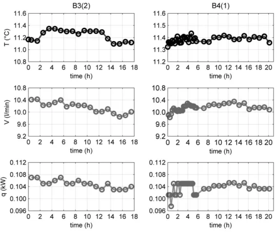
Figure 11 presents the depth-average temperature evolution for B3 and B4, considering the whole borehole length. Temperature fluctuates around a mean value of 11.24±0.13 °C for B3 and 11.38±0.06 °C for B4. Calculating the depth-average temperature for a depth greater than 18 m (thermally stable zone) results in a slightly lower temperature of 0.03 °C for B3 and of 0.05 °C for B4. The measured profiles during water circulation are highly influenced by the water-ground interaction, minimizing the air temperature effects. The temperature
24 fluctuations observed during the whole test duration might be partially attributed to the pump work and flow rate oscillations.
Figure 11 - Depth-average ground temperature (fiber optics) (top), average volumetric flow rate (middle) and average pump work (bottom) in B3 and B4
Figure 12 presents the ground temperature as estimated by the four different temperature data sets: one recorded at the undisturbed state at the beginning of the test and three during water circulation in the pipe loops. The fiber optic measurements at the beginning of the test are considered as the reference values, since the calibrated fiber optic profiles are not biased by ambient air temperature conditions. The fiber optic measurements provide a more accurate estimation of the ground temperature (overestimation less than 0.2 °C) than the pipe-inlet/outlet measurements and result to an overestimation of the maximum extracted power
25 and of the COP of less than 2.5%, for high ambient air temperature during the test (B1, B3(2)). For low ambient air temperature, all the measurements result in a small overestimation of the ground temperature (<0.06 °C). As also presented in the water measurements analysis (section 3.1.2.1), this small overestimation can be attributed to the accuracy of the measurements.
Figure 12 - Comparison of estimated ground temperature based on data (time-average values) during water circulation (mean air temperature: 15.65 °C for B1, 13.45 °C for B3(2) and 4.70 °C for B4(1))
3.2 Investigating the temperature anomaly through analytical and numerical modelling The temperature profiles measured before the in-situ tests (section 3.1.1) are further studied in this section by analytical and numerical modelling. It is investigated if the measured temperature anomaly could be attributed to the heating of the subsurface through the SEGI basement and the feeder pipe shell.
26 Figure 13 presents the ground temperature estimated analytically for the Sart-Tilman area. The ground temperature in the upper 18 m varies during the year, since it is influenced by the seasonal weather conditions. At the depth of 18 m, the ground temperature reaches 9.1 °C which is close to the average annual air temperature of Sart-Tilman area (8.9 °C). Below this depth temperature increases with depth due to the geothermal gradient effect. Based on the fiber optics measurements, the influence of the air temperature is also limited in the upper 18 m. However, at the depth of 18 m the measured temperature is 3 °C higher in the boreholes and 1 °C higher in the well than the corresponding analytically estimated temperature. Moreover, temperature decreases through depth in the four boreholes, opposite to the geothermal gradient effect.
Figure 13 - Undisturbed ground temperature estimated analytically for the Sart-Tilman area
Figure 14 presents numerical results of the ground surrounding the four boreholes. The initial ground temperature (before the existence of structures, in 1970) is dominated by the geothermal gradient effect. The heating of the ground, through the pipe shell (150 W/m
27 length) and through the SEGI basement (4 W/m² based on the numerical results) modifies the temperature gradient at the location of the boreholes down to a depth of 100 m after 20 years (1990). The heating effect becomes progressively evident at greater depth, reaching a depth of 130 m after 45 years (2015). Moreover, the curvature of the temperature profiles is clearly evolving with time, with the increasing amount of heat added to the ground. The depth-average temperature of the ground which is not influenced by the weather conditions (below 18 m) increases at a mean rate of 0.03 °C/year for the first 45 years (1970-2015).
28 In terms of spatial impact, the modelled temperature in B1 is lower in the upper 18 m compared to the other three boreholes (Figure 15), as also observed in the fiber optic profiles. The lower temperature can be attributed to the distance of each borehole from the feeder pipe, which is located at an average depth of 2.5 m. Given that B2, B3 and B4 are 4 m closer to the feeder pipe than B1, the heat loss effect from the feeder pipe will be more enhanced in the location of these three boreholes. Below 18 m, the temperature profile given by the numerical model is in good agreement with the experimental one. The numerical results satisfactory predict the depth-average temperature in the period 2013-2015 (mean overestimation of 0.11 °C, Table 4). It should be noted that based on the numerical results the ground temperature increases at very low rate of 0.017 °C/year for the two-year measurement period. This low temperature increase is not clearly evident in the fiber optics measurements, given the short measurement period in combination with the accuracy of the fiber optic measurements (section 2.2.1).
Figure 15 - Experimental and numerical results of the ground temperature at the location of the four boreholes
29 Table 4 - Comparison of experimental and numerical results for the depth-average ground temperature
(18 m - 100 m) at the undisturbed state
Fiber optics (°C) Numerical model (°C) year 2013 2014 2015 2013 2014 2015 B1 11.00 10.99 11.05 11.13 11.16 11.17 B2 10.97 10.98 11.03 11.05 11.08 11.09 B3 10.83 10.95 11.01 11.03 11.05 11.06 B4 11.03 10.94 10.96 11.05 11.08 11.09
Figure 16 presents the numerical results and the temperature measurements in the well. According to the numerical results, the heat loss through the feeder shell modifies the temperature field at the location of the well, despite its great distance to the feeder (27 m). Below 20 m, temperature is almost invariant with depth and reaches a value of 10.1 °C in 2016, which is in good agreement with the corresponding measured temperature. Given the good agreement between the temperature measurements and the numerical results, the measured temperature profiles can be attributed to the heat loss through the surrounding structures.
30 3.3 Design in urbanised areas
Table 5 shows the depth-average temperature at the location of the boreholes during time and the impact on the design for heating dominated systems. The maximum extracted power increases by 9% after 10 years of the feeder operation and by 17% after 50 years. The ground temperature increase has also a noticeable effect on the heat pump COP (increase of 6% after 50 years).
Moreover, the urbanisation effect results in a decreasing temperature with depth, which indicates that short BHEs can be characterised by a higher capacity (maximum extracted power per m length) and can result in an increased heat pump COP compared to long BHEs. Table 6 summarizes different proposed configurations (number and length of BHEs) for various heat demands considering the temperature profile at the location of the boreholes for 2014 and a uniform ground thermal conductivity. The extracted power for each proposed length was defined based on the corresponding depth-average ground temperature and the MCS 022 (MIS 3005 [13]) look-up tables. The heat pump COP for various BHE lengths is presented in Figure 17, considering the temperature of the cold reservoir equal to the corresponding depth-average ground temperature. Among the different configurations, groups of short BHEs (~40 m length) result in reduced required total length up to 9% and relative COP increase of 4%.
31 Table 5 - Numerical results of the depth-average temperature evolution at the location of the BHEs,
maximum extracted power and coefficient of performance of the heat pump year T (°C) Q* (W/m) COP** 1970 9.6 45.3 5.2 1980 10.5 49.3 5.3 1990 10.9 51.0 5.4 2000 11.1 52.0 5.4 2020 11.4 53.1 5.5
* MCS 022 (MIS 3005 [13]), 1200 FLEQ run hours ** n=0.5, TH=40 °C
Table 6 - Proposed configurations for various heat demands
10 kW heat demand 15 kW heat demand 20 kW heat demand number x length
(total length decrease*)
number x length (total length decrease*)
number x length (total length decrease*) 1 x 193 m (-) 2 x 145 m (-) 2 x 193 m (-) 2 x 95 m (2%) 3 x 95 m (2%) 3 x 128 m (1%) 3 x 61 m (5%) 4 x 69 m (5%) 4 x 95 m (2%) 4 x 44 m (9%) 5 x 54 m (7%) 5 x 75 m (3%) 6 x 44 m (9%) 6 x 61 m (5%) 7 x 52 m (6%) 8 x 44 m (9%) * with regard to the deeper BHE proposition
32 Figure 17 - Coefficient of performance of the heat pump for varying BHE length (n=0.5, TH=40 °C)
In practise, the number and length of the required BHEs is proposed based on the results of a TRT in a pilot BHE installed in-situ. The undisturbed ground temperature gradient can be obtained by lowering a temperature sensor inside the pilot BHE pipes, which is a cost effective and easy to implement. Figure 18 shows the effect of a negative ground temperature gradient on the total length and the COP for groups of short BHEs, compared to BHEs of 100 m long. Groups of short BHEs (length < 40 m) are particularly advantageous for temperature gradient lower than -0.05 °C/m, since the total required length decreases by more than 10% and the heat pump COP increases by more than 5%. The installation and operation costs savings are in the order of 4000 € and 100 €/year respectively for a temperature gradient of -0.05 °C/m and heat demand of 15 kW (Table 7).
33 Figure 18 - Effect of undisturbed temperature gradient on the total BHE length (top) and the heat pump COP (bottom) for groups of short BHEs, compared to a reference BHE length of 100 m (MCS
022, n=0.5, TH=40 °C)
Table 7 - Installation and heat pump operation costs (grad.: -0.05 °C/m, heat demand: 15 kW) run hours
configuration installation cost* (€) heat pump operation cost** (€/year)
1800 3 x 110 m 33000 1208 7 x 42 m 29400 1142 2400 4 x 92 m 36800 1610 8 x 41 m 32800 1522 3000 4 x 101 m 40400 2013 8 x 45 m 36000 1904 *100 €/m BHE **0.25 €/kWh
34 4. Discussion
In the presented numerical model, the average annual heat loss through the feeder shell (150 W/m length) was assumed equal to the one of only one year (2011). The lack of measured data increases the uncertainty of the average annual heat loss for the investigated period of 60 years. Figure 19 (left) shows the influence of this parameter to the temperature at the location of the boreholes. The slope of the temperature profile and the depth-average temperature increase with increasing heat loss. However, for the investigated range, the depth-average temperature (18 m -100 m depth) does not differ significantly from the corresponding measured value (DT<0.3 °C). The temperature at the surface of the SEGI building was fixed equal to the one measured at the basement of the building during a few weeks in 2015. This could differ from the average annual temperature in the basement. Moreover, this temperature was assumed equal to the one at the interface between the basement's plate and the ground, without taking into account the plate's geometry and thermal properties. However, the sensitivity analysis presented in Figure 19 (right) indicates that a more accurate simulation would not significantly modify the temperature profiles at the location of the boreholes.
35 Figure 19 - Influence of the applied heat loss through the feeder shell (left) and of the fixed temperature at the SEGI surface (right) on the ground temperature at the location of the boreholes
In this model, the ground was considered an homogeneous, isotropic medium. Simulating the different ground layers with varying thermal behaviour could modify the slope of the temperature profiles. Moreover, the boundary conditions applied at the ground surface are simplified without taking into account wind convection effects, solar radiation effect and the geometry or thermal characteristics of the asphalt layers. Taking into account these effects in advanced boundary conditions, as well as the air temperature variation through the year, can allow a more accurate simulation of the temperature field evolution with time, especially in the thermally unstable zone which would be of high interest for horizontal closed-loop geothermal systems. In this case, it should also be considered that the thermal conductivity of the top layers, which are characterised by a different geology (sand and gravel) than the remaining part of the borehole (sandstone, shale, siltstone), could vary significantly from the mean thermal conductivity estimated based on the TRT results.
36 5. Conclusions
The preliminary phase of a TRT (fluid circulation in the pipe loops) allows to determine the depth-average ground temperature. The accuracy of this procedure depends on the accuracy of the measurement equipment, the heat added to the circulating fluid due to the pump work and the thermal interaction between the fluid and the ambient air. The latter can result in a significant error in the ground temperature estimation (overestimation up to 1.7 °C in this case study) with a noticeable effect on the maximum extracted power of the BHE and of the heat pump COP (overestimation up to 14% and 6% respectively in this case study). To limit the error in the COP and the extracted power to less than 5%, the error in the undisturbed temperature estimation should not exceed ±1.5 °C and ±0.6 °C respectively. In the case of a low ambient air temperature, the corresponding error in the estimated ground temperature is expected to be lower, since the final heat extracted by the fluid will be reduced due to the pump work added heat. Borehole logging measurements during the test seem to be less affected by the air-water thermal interaction and provide a more accurate estimation of the undisturbed temperature. Given the importance of the undisturbed ground temperature for the design of closed-loop systems, it is recommended to insulate not only the pipes but also the test rig. This allows avoiding a significant overestimation of the extracted power of the BHEs, in the case of high ambient air temperature.
In this case study, the undisturbed ground temperature profiles are characterised by an elevated temperature and a negative temperature gradient. These profiles can be the result of the ground heating by structures located close to the boreholes (feeder pipe at a distance of 6.6 m and a building at a distance of 15 m), as verified by the numerical model analysis compared to the analytical predictions. The heat loss into the subsurface, through the feeder pipe shell (150 W/m length ) and through the SEGI basement (4 W/m²), has a significant
37 effect on the design of BHEs. After 10 years of the feeder operation, the maximum extracted power at the location of the boreholes increases by 9% and after 50 years by 17%.
In urbanised areas, configurations of short BHEs (length < 40 m) could be economically advantageous (decreased installation and operation costs) compared to long BHEs, especially for temperature gradient lower than -0.05 °C/m. In real applications, the temperature gradient could be revealed by temperature monitoring along a pilot BHE. Apart from fiber optic cables, the temperature distribution through depth can be fairly obtained by lowering a temperature sensor into the pipe and measuring the temperature at intervals. This is a widely applicable, cost-effective and easy-to-implement approach and does not require preinstalled equipment. The number and length of the required BHEs can be then optimised, by taking into advantage the negative temperature gradient caused by the urbanisation effect.
In urbanised areas, the heat loss through building foundations and underground structures (feeder pipes, sewage pipes etc.) recharges the geothermal reservoir. This is a continuous phenomenon which can affect the long-term behaviour of the geothermal systems. Given that the ground temperature field is significantly affected close to the structures, the case of energy piles would be particularly interesting, since they are located underneath the building and are usually shorter than BHEs. The heat loss into the subsurface can counteract the progressive cooling of the ground during the operation of the system. Moreover, the thermal performance of the system can improve during its life span, affected not only by the operation of existing structures, but also by new structures in the area. Taking this effect into account can contribute to a sustainable geothermal reservoir management in a city scale.
38 Acknowledgements
The work undertaken in this paper is supported by the Walloon Region project Geotherwal n° 1117492 and the F.R.S.-FNRS F.R.I.A. fellowship of Georgia Radioti. We also would like to thank the University service ARI for their support in the installation of the BHEs as well as our partners in the project, the ULB (Université Libre de Bruxelles) and the companies OREX and Geolys. We thank the company REHAU for providing the pipes and the commercial grouting materials.
References
[1] Kaushal, M. (2017). Geothermal heating/cooling using ground heat exchanger for various experimental and analytical studies: Comprehensive review. Energy and Buildings, 139, 634-652
[2] Lund, J.W., Freeston, D.H. and Boyd T.L. (2011). Direct utilization of geothermal energy 2010 worldwide review. Geothermics, 40 (3), 159-180
[3] Lucia, U., Simonetti, M., Chiesa, G. and Grisolia, G. (2017). Ground-source pump system for heating and cooling: Review and thermodynamic approach. Renewable and Sustainable
Energy Reviews, 70, 867-874
[4] Florides, G. and Kalogirou, S. (2007). Ground heat exchangers-A review of systems, models and applications. Renewable Energy, 32 (15), 2461-2478
[5] Villarino, J.I., Villarino, A. and Fernández, F.A. (2017). Experimental and modelling analysis of an office building HVAC system based in a ground-coupled heat pump and radiant floor. Applied Energy, 190, 1020-1028
[6] Buckley, C., Pasquali, R., Lee, M., Dooley, J. and Williams, T.H. (2015). 'Ground Source
39 [7] Self, S.J, Reddy, B.V. and Rosen, M.A. (2013). Geothermal heat pump systems: Status review and comparison with other heating options. Applied Energy, 101, 341-348
[8] Noorollahi, Y., Gholami Arjenaki, H. and Ghasempour, R. (2017). Thermo-economic modeling and GIS-based spatial data analysis of ground source heat pump systems for regional geothermal mapping. Renewable and Sustainable Energy Reviews, 72, 648-660 [9] Han, C. and Yu, X. (2016). Sensitivity analysis of a vertical geothermal heat pump system.
Applied Energy, 170, 148-160
[10] Blum, P., Campillo, G. and Kölbel, T. (2011). Techno-economic and spatial analysis of vertical ground source heat pump systems in Germany. Energy, 36 (5), 3002-3011
[11] Recknagel, H., Sprenger, E., Schramek, E.-R. (2007). Génie climatique [Taschenbuch
für Heizung und Klimatechnik], translated in French by Bodson, A., Caradec, C., Pastureau,
S. and Petit, N., Eds. Dunod, Paris
[12] Kavanaugh, S. and Rafferty, K. (2014). Geothermal Heating and Cooling: Design of
Ground-Source Heat Pump Systems. ASHRAE, Atlanda, Georgia
[13] MIS 3005 (2008): Requirements for MCS contractors undertaking the supply, design,
installation, set to work, commissioning and handover of microgeneration heat pump systems. Department of Energy and Climate Change, London
[14] Dehkordi, S.E. and Schincariol, R.A. (2014). Effect of thermal-hydrogeological and borehole heat exchanger properties on performance and impact of vertical closed-loop geothermal heat pump systems. Hydrogeology Journal, 22, 189-203
[15] Kurevija, T., Vulin D. and Macenić, M. (2014). Impact of geothermal gradient on ground source heat pump system modeling. Rudarsko Geolosko Naftni Zbornik, 28, 39-45 [16] Spitler, J.D. and Gehlin, S. (2015), Thermal response testing for ground source heat
40 pump systems-An historical review. Renewable and Sustainable Energy Reviews, 50, 1125-1137
[17] Acuña, J., Morgesen, P. and Palm, B. (2009). Distributed thermal response test on a U-pipe borehole heat exchanger. In: EFFSTOCK Conference Proceedings 2009, Stockholm, Sweden, 14-17 June
[18] Loveridge, F., Holmes, G., Powrie, W. and Roberts, T. (2013). Thermal response testing through the Chalk aquifer in London, UK. Proceedings of the Institution of Civil Engineers:
Geotechnical Engineering, 166 (2), 197-210
[19] Gehlin, S.E.A. and Nordell, B. (2003). Determining undisturbed ground temperature for thermal response test. ASHRAE Transactions, 109, 151-156
[20] Choi, W. and Ooka, R. (2015). Interpretation of disturbed data in thermal response tests using the infinite line source model and numerical parameter estimation method. Applied
Energy, 148, 476-488
[21] Bandos, T.V., Montero, A., Fernádez de Córdoba, P. and Urchueguía, J. F. (2011). Improving parameter estimates obtained from thermal response tests: Effect of ambient air temperature variations. Geothermics, 40 (2), 136-143
[22] Singorelli, S., Bassetti, S., Pahud, D. and Kohl, T. (2007). Numerical evaluation of thermal response tests. Geothermics, 36, 141-166
[23] Popiel, C.O., Wojtkowiak, J. and Biernacka, B. (2001). Measurements of temperature distribution in ground. Experimental Thermal and Fluid Science, 25, 301-309
[24] Bayer, P., Rivera, J., Schweizer, D., Schärli, U., Blum, P. and Rubach, L. (2016). Extracting past atmospheric warming and urban heating effects from borehole temperature profiles. Geothermics, 64, 289-299
[25] Menberg, K., Bayer, P., Zosseder, K., Rumohr, S. and Blum, P. (2013). Subsurface urban heat islands in German cities. Science of the Total Environment, 442, 123-133
41 [26] Zhu, K., Blum, P., Ferguson, G., Balke, K.D. and Bayer, P. (2010). The geothermal potential of urban heat islands. Environmental Research Letters, 5, 044002
[27] Banks, D., Gandy, C.J., Younger, P.L., Withers, J. and Underwood, C. (2009). Anthropogenic thermogeological 'anomaly' in Gateshead, Tyne and Wear, UK. Quarterly
Journal of Engineering Geology and Hydrogeology, 42, 307-312
[28] Liebel, H.T., Huber, K., Frengstad, B.S., Ramstad, R.K. and Brattli, B. (2011). Temperature footprint of a thermal response test can help to reveal thermogeological information. Norges geologiske undersøkelse Bulletin, 451, 20-31
[29] Yamano, M., Goto, S., Miyakoshi, A., Hamamoto, H., Lubis R.F., Monyrath, V. and Taniguchi, M. (2009). Reconstruction of the thermal environment evolution in urban areas from underground temperature distribution. Science of the Total Environment, 407, 3120-3128
[30] Ferguson, G. and Woodbury, A.D. (2007). Urban heat island in the subsurface.
Geophysical research letters, 34 (23), L23713
[31] Rivera, J., Blum, P. and Bayer, P. (2015). Analytical simulation of groundwater flow and land surface effects on thermal plumes of borehole heat exchangers. Applied Energy, 146, 421-433
[32] Rivera, J., Blum, P. and Bayer, P. (2016). Influence of spatially variable ground heat flux on closed-loop geothermal systems: Line source model with nonhomogeneous Cauchy-type top boundary conditions. Applied Energy, 180, 572-858
[33] Rivera, J., Blum, P. and Bayer, P. (2017). Increased ground temperatures in urban areas: Estimation of the technical geothermal potential. Renewable Energy, 103, 388-400
[34] Radioti, G., Charlier, R., Nguyen, F. and Radu, J.-P. (2013). Thermal Response Test in Borehole Heat Exchangers Equipped with Fiber Optics. In: Proceedings, International
42
Workshop on Geomechanics and Energy: The Ground as Energy Source and Storage, EAGE,
Lausanne, Switzerland, 96-100
[35] Radioti, G., Delvoie, S., Sartor, K., Nguyen, F. and Charlier, R. (2015). Fiber-optic temperature profiles analysis for closed-loop geothermal systems: a case study. In:
Proceedings, Second EAGE Workshop on Geomechanics and Energy: The Ground as Energy Source and Storage, EAGE, Celle, Germany
[36] Radioti, G., Delvoie, S., Charlier, R., Dumont, G. and Nguyen, F. (2016a). Heterogeneous bedrock investigation for a closed-loop geothermal system: A case study.
Geothermics, 62, 79-92
[37] Radioti, G., Delvoie, S., K. Sartor, Nguyen, F. and Charlier, R. (2016b). Fiber-optic temperature measurements in closed-loop geothermal systems: a case study in heterogeneous bedrock. In: Proceedings of 1st International Conference on Energy Geotechnics ICEGT 2016, Kiel, Germany
[38] Gehlin, S. (2002). Thermal Response Test - Method, Development and Evaluation. Doctoral dissertation, Luleå University of Technology, Sweden
[39] Hermans, T., Nguyen, F., Robert, T. and Revil, A. (2014). Geophysical Methods for Monitoring Temperature Changes in Shallow Low Enthalpy Geothermal Systems. Energies, 7, 5083–5118
[40] Hausner, M.B, Suarez, F., Glander, K.E., van de Giesen, N., Selker, J.S. and Tyler, S.W. (2011). Calibrating single-ended fiber-optic raman spectra distributed temperature sensing data. Sensors, 11, 10859-10879
[41] Tinti, F. (2012). The probabilistic characterization of underground as a tool for the
optimization of integrated design of shallow geothermal systems. Doctoral dissertation,
43 [42] Petitclerc, E. and Vanbrabant, Y. (2011). Développement de la plate-forme
Géothermique de la Wallonie. Rapport final, DGO4. Retrieved online:
http://energie.wallonie.be/fr/la-geothermie-profonde.html?IDC=6173
[43] Climate-data.org: Climate data for cities worldwide. Last accessed 15-10-2015, http://en.climate-data.org/
[44] Charlier, R., Radu, J.-P. and Collin, F. (2001). Numerical modelling of coupled transient phenomena. Revue Française de Génie Civil, 5(6), 719-741
[45] Collin, F., Li, X.L., Radu, J.-P. and Charlier, R. (2002). Thermo-hydro-mechanical coupling in clay barriers. Engineering Geology, 64, 179-193
[46] Sartor, K., Quoilin, S. and Dewallef, P. (2014). Simulation and optimization of a CHP biomass plant and district heating network. Applied Energy, 130, 474–483
[47] Smolarczyk, U. (2003). Geotechnical Engineering Handbook, Vol.2: Procedures, Berlin [48] Nguyen, D. and Lanini, S. (2012). Projet Solargeotherm: modélisations numeériques de
transferts thermiques dans le dispositif souterrain d’échange de