1. Introduction
Located at the interface between terrestrial ecosystems and water resources such as water courses and shallow water tables, wetlands are a pivotal part of the drainage network of a watershed. Consequently, they affect the routing of overland and subsurface flows through modification of hydrological processes, namely increased evapotranspiration, water storage and groundwater recharge (Bullock and Acreman, 2003). These interactions have led researchers and land planners to attribute some hydrological services to wetlands, such as low flow support and high flow attenuation. As defined by Roche (1986), low flows refer to the lowest annual flow of a water course at a given point in space. To characterize low flows, various hydrological indicators have been defined, taking into account the return period: 2-year minimum flow over 7 days, 10-year minimum flow over 7 days, 5-year minimum flow over 30 days, etc. On the other hand, high flows are defined as the peak flow within a specific return period, typically 2-, 20- or 100-year maximum flows.
In the last century, anthropic activities such as agricultural and urban development have induced major land cover changes; affecting the hydrological regime of watersheds (St-Hilaire et al., 2015; Salvadore et al., 2015; Savary et al., 2009; DeFries and Eshleman, 2004). Agricultural impacts on hydrological processes are mostly associated with artificial drainage, which alters the water volume and timing of runoff (e.g.: Muma et al., 2016; Blann et al., 2009). For example, in the Redwood basin, a Midwestern United States agricultural basin, the total area of soybean (associated with the installation of extensive subsurface drainage tiles) increased from 15% to 40% between 1971 and 2002, and this led to an increase in mean annual flows from 2.3 m3/s to 6.0 m3/s (Foufoula-Georgiou et al., 2015). Similarly, Muma et al. (2016) showed that subsurface drainage increased base and total flows, and decreased peak flows of an intensively farmed 2.4 km2 watershed (90% in cropland with 30% of the watershed area tile-drained). As for the impacts of urban development on hydrology, characterized by increasing impervious surfaces, they range from affecting water supply by limiting infiltration, to changes in water demand in response to an increased population (DeFries and Eshleman, 2004; Diem et al., 2018). In the Atlanta metropolitan area, impervious cover of the Big Creek and Suwanee Creek watersheds increased from 8 to 17% and from 9 to 21% respectively, between 1992 and 2011, inducing an increase in the annual stream flow of 26% (Diem et al., 2018).
Anthropic activities have also led to the draining of wetlands and modification of the land cover within their drainage area (Zedler and Kercher, 2005; Brinson and Malvarez, 2002). At the global scale, wetland losses estimations are up to 87% and the yearly rate of these losses accelerated between -0.68 to -0.69% in the 1970s to between -0.85 to -1.60% in the 2000s, depending on the region (Davidson, 2014; Ramsar Convention on Wetland, 2018). In all likelihood, these losses have had an
impact on the hydrological services provided by wetlands such as low flow support and high flow attenuation. This should support the development of safeguarding actions and policy decisions to protect and restore wetlands. Watson et al. (2016) recently studied the flood mitigation service provided by floodplains and wetlands in the Otter Creek watershed, Middleburry, VT, and concluded that they have contributed to the reduction of flood damages on manmade infrastructures by 54% to 78% for 10 major events, including Tropical Storm Irene.
Hydrological models such as the Soil and Water Assessment Tool (SWAT; see Supplementary material for a list of abbreviations), the Soil and Water Integrated Model (SWIM) and HYDROTEL have been used to assess the impact of wetlands on selected hydrological processes at the watershed scale (Liu et al., 2018; Liu et al., 2008; Wang et al., 2008; Wu and Johnston, 2008; Wang et al., 2010). For example, Wang et al. (2010) used SWAT and the hydrologically equivalent wetland (HEW) concept to assess the effects of wetland restoration and conservation for two watersheds in Manitoba and Minnesota. They found that the first 10-20% losses of wetlands conducted to a measurable increase in peak discharge and that 50-80% of wetlands would need to be restored in order to reduce it substantially. More recently, the impact of wetlands on high and low flows was assessed using the hydrological modelling platform PHYSITEL/HYDROTEL; adapting the model to explicitly account for wetlands (Fossey et al., 2015; including a complete description of the integration of modules to HYDROTEL and related equations). For two watersheds (Quebec, Canada), the authors showed that wetlands can reduce high flows between 6 and 18 %, while increasing low flows between 22% and 75% (Fossey and Rousseau, 2016a). The development of hydrological models has provided researchers with a powerful framework for quantifying the hydrological services supplied by wetlands and opened new research avenues to explore the impact of wetlands on the hydrological regime of a watershed under current and future climate conditions (Fossey and Rousseau, 2016a, 2016b). Given this framework, in this paper, we explore, using a case study, the impact of land cover changes between 1978 and 2014 on the hydrological services provided by wetlands on low flows and high flows at the sub-watershed scale of a Canadian watershed under temperate climate conditions. This study builds on the recent work of Blanchette et al. (2018), which has shown using Landsat archive images that wetland areas in the St. Charles River watershed (Quebec, Canada) have decreased by 15% between 1978 and 2014. Moreover, taking advantage of the availability of various historical land cover scenarios developed, we explore whether the use of different land cover maps, representative of the dates of operation of each hydrometric station, could improve the calibration of HYDROTEL.
2. Materials and methods
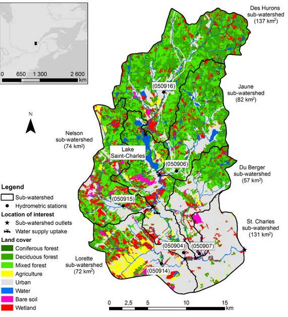
The St. Charles River watershed is located on the north shore of the St. Lawrence River, in southern Quebec, Canada. The river drains a total area of 554 km2, with altitudes ranging from 4 to 844 m above mean sea level (Natural Resources Canada, 2013). The mean annual total precipitation and mean temperature for the 1969-2016 period were 1329 mm (31% as snow) and 3.9°C (12.2°C from March 21 to September 20, -4.5°C from September 21 to March 20), respectively, whereas the mean annual stream flow was 8.1 m3/s at hydrometric station 050904 (Fig. 1; Ministry of Sustainable Development, the Environment and the Fight Against Climate Change, 2017).
The hydrographic network is composed of six main tributaries; dividing the watershed into major sub-watersheds (Fig. 1). Lake St. Charles (3.6 km2) is located at the center of the watershed and is replenished mostly by the Des Hurons River (82% of average annual inflows; APEL, 2015). The lake also acts as a drinking water reservoir for approximately 300,000 citizens of Quebec City. The drinking water treatment plant (i.e., uptake) is located 11 km downstream of the lake.
Based on the comparison of the 1978 and 2014 land cover maps (Table 1), wetland areas decreased from 12.5% (69.1 km2) to 10.6% (58.5 km2), representing a decrease of 15% at the St. Charles watershed scale. However, the changes in wetland areas at a finer scale highlight different dynamics among the sub-watersheds (Table 2). While the Jaune River sub-watershed had the most important decrease in wetland area (-44%), the Des Hurons and the water intake sub-watersheds also had wetland cover loss; decreasing by 40% and 30%, respectively. Such losses suggest that these sub-watersheds would also be the most impacted in terms of losses of hydrological services. Moreover, knowing that these three watersheds, mostly located in the upper part of the watershed, have a higher proportion of isolated wetlands, in contrast with riparian wetlands, their loss in hydrological services could even be stronger. This combination of spatial attributes has proven to play a key role in hydrological services, as illustrated by Fossey et al. (2016). Inversely, the Lorette sub-watershed underwent an increase in wetland areas from 10.1% (7.3 km2) to 14.7% (10.6 km2), where agriculture was dominant in the 1970s and fallow land could have naturally evolved into a wetland state (e.g.: wet meadows), therefore increasing their hydrological services.
Fig. 1. Location of the St. Charles River watershed, including sub-watershed delineation, hydrometric stations, locations of interest and 2014 land cover map (Blanchette et al., 2018). The numbers in parentheses refer to the ID of the hydrometric stations used for calibration.
Land cover classes 1978 2014 Wetland 12.5 (69.1) 10.6 (58.5) Forest 50.9 (281.8) 51.4 (284.8) Water 1.7 (9.6) 2.2 (11.9) Agriculture 20.3 (112.4) 3.5 (19.3) Urban 14.0 (77.5) 31.0 (171.8) Bare soil 0.6 (3.5) 1.4 (7.7)
Table 1. Percentage (numbers in parentheses refer to the area in km2) of land cover classes for the entire St. Charles watershed for the 1978 and 2014 land cover scenarios.
Sub-watershed Area (km2) 1978 2014 I R T I R T Des Hurons 137 10.4 (18.8) 4.4 (8.3) 14.8 (27.1) 6.0 (13.5) 2.9 (7.3) 8.9 (20.8) Jaune 82 8.2 (18.4) 5.7 (9.2) 14.0 (27.6) 4.6 (11.4) 3.2 (8.3) 7.8 (19.7) Nelson 74 14.4 (27.8) 4.7 (8.8) 19.1 (36.6) 11.2 (25.1) 6.5 (15.4) 17.6 (40.5) Lorette 72 5.5 (14.4) 4.6 (5.5) 10.1 (19.9) 8.2 (17.5) 6.5 (10.0) 14.7 (27.5) Du Berger 57 6.5 (18.1) 2.6 (5.5) 9.1 (23.6) 4.8 (15.1) 4.4 (10.8) 9.3 (26.0) Water intake 349 10.7 (20.8) 5.2 (8.8) 15.9 (29.6) 6.8 (16.2) 4.3 (9.8) 11.1 (25.9) Total 554 8.3 (17.2) 4.2 (6.9) 12.5 (24.1) 6.2 (15.3) 4.4 (9.4) 10.6 (24.7)
Table 2. Changes, between 1978 and 2014, of the area (%) occupied by wetlands and, in parentheses, their drainage area, for each sub-watershed. The drainage area of a wetland is calculated by processing the flow accumulation matrix in PHYSITEL (Fossey et al., 2015) and refers to the area drained by the wetland. I: isolated wetlands, R: riparian wetlands, T: total wetlands (the discrepancies in the total % of area are due to rounding effects).
2.2 Data input in PHYSITEL and processing steps
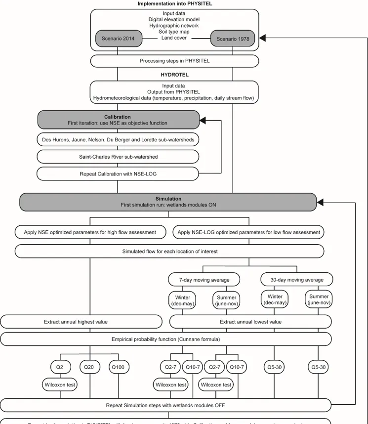
PHYSITEL is a specialized geographic information system (GIS) that was developed to support the implementation of distributed hydrological models (Turcotte et al., 2001; Rousseau et al., 2011; Noël et al., 2014). It requires the following input data (Fig. 2): (i) a digital elevation model (DEM), (ii) a hydrographic network, (iii) a soil type map, and (iv) a land cover map. The DEM and the river network were extracted from GeoGratis (http://geogratis.cgdi.gc.ca/). For this study, the resolution of the DEM
was 20 m, whereas the river network was extracted at a resolution of 1:50,000 (Natural Resources Canada, 2013). Prior to importation in PHYSITEL, the river network was filtered according to the following steps: (i) removal of intermittent river segments, segments located in waterbodies and segments/waterbodies unconnected to the river network, (ii) conversion of undesired loops to river segments by choosing the most plausible water pathway, (iii) merging water bodies made of multiple polygons into a single one, (iv) merging of all segments, (v) fragmentation of the river network into the desired location of nodes, and finally, (vi) removal of river segments smaller than one DEM cell (20 m). The final river network contained 434 river segments with a mean length of 900 m. A soil type map was used to identify the soil textures, based on the percentages of loam, clay, and sand (http://sis.agr.gc.ca/cansis/nsdb/slc/index.html; Soil Landscapes of Canada Working Group, 2010; Rawls and Brakensiek, 1989). Two different land cover maps (i.e., 1978 and 2014), generated using the same methodology (Blanchette et al., 2018), were used in this study, resulting in two different modelling projects.
Once the data were imported, the following processing steps were performed in PHYSITEL: (i) conversion of the river network into a raster format, (ii) calculation of the slope and flow direction of each cell (D8-LTD algorithm; Orlandini et al., 2003), (iii) identification of the cell corresponding to the outlet of the watershed, (iv) delineation of the watershed (using a recursive approach), (v) subdivision of the watershed into 1505 relatively homogeneous hydrological units (RHHUs; with a mean area of 0.83 km2 and a standard deviation of 2.14 km2), namely hillslopes, (vi) identification of the dominant soil type and percentages of different land covers for each RHHU, (vii) recognition of the wetland class from the land cover map, (viii) wetland surface and drainage area calculation, (ix) distinction between isolated and riparian wetlands, and (x) export to HYDROTEL. Because of standard data formats and universal data types, output data can be used by a wide range of distributed hydrological models.
2.3 HYDROTEL
2.3.1 Model description and data input
HYDROTEL (for complete descriptions of the governing equations of each computational module, see Fortin et al., 2001; Turcotte et al., 2003; Turcotte et al., 2007; Bouda et al., 2012; Bouda et al., 2014) is a distributed, process-based, continuous hydrological model which can be run at either daily or sub-daily time steps. The model is built around six computational modules performing various tasks and calculations: (i) interpolation of precipitations over the watershed at the scale of each RHHU, (ii) accumulation and melt of snowpack, (iii) potential evapotranspiration, (iv) vertical water balance, (v) surface/subsurface flow routing, and (vi) river flow routing. The water mass balance is computed at the RHHU level.
Besides the data processed by PHYSITEL, HYDROTEL requires meteorological data (daily precipitation, maximum and minimum temperatures) and hydrometric data (daily stream flows) for calibration purpose. A meteorological data set was built using daily precipitation and temperatures recorded by Environment and Climate Change Canada and Quebec City. For stream flows, a network of hydrometric stations has been recording water levels at different locations within the St. Charles River watershed, with one of the stations (050904, Fig. 1) in operation since 1969 (Ministry of Sustainable Development, the Environment and the Fight Against Climate Change, 2017).
2.3.2 Model calibration and validation
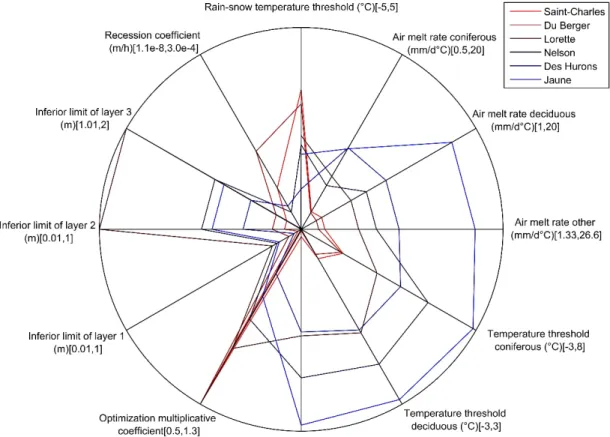
The dynamically dimensioned search (DDS; Tolson and Shoemaker, 2007) algorithm was used to calibrate the most sensitive parameters of the model, while the least sensitive parameters were fixed based on previous knowledge about the model (Supplementary material). DDS was designed to solve calibration problems with many parameters and is therefore particularly well suited for distributed hydrological models like HYDROTEL. The maximum number of iterations and the lower and upper bounds of each calibrated parameter values are required to initiate the automated calibration. Given this information, the algorithm searches for a global optimum in the first iterations and focuses on a local optimum as the number of iteration approaches the maximum number defined by the user.
For this project, the set of parameter values having the highest Nash-Sutcliffe efficiency criterion (NSE; Nash and Sutcliffe, 1970) was retained for high flows and the highest Nash-Sutcliffe efficiency calculated on logarithmic flows (NSE-LOG) was retained to assess low flows (Fig. 2). In both cases, DDS ran a total of 250 iterations. The Kling-Gupta efficiency criterion (KGE) (Gupta et al., 2009), the percent bias (P-Bias) (Yapo et al., 1996) and the root mean square error (RMSE) (Singh et al., 2005), which are goodness-of-fit indicators (GOFIs) extensively described in the literature and frequently used
in various calibration procedures of hydrological models, were also used to assess the calibration results, along with the performance rating scale developed by Moriasi et al. (2007). To avoid model initialization errors, a one-year spin-off period was considered for calculation of the GOFIs. The calibration was executed for a time interval of four to six years towards the end of the operation period of each station. The validation considered the entire period of operation. For the Lorette hydrometric station exclusively, which was only operated for four years, no validation was carried out. The Des Hurons, Jaune, Nelson, Du Berger and Lorette sub-watersheds were first calibrated independently. The St. Charles sub-watershed was calibrated taking into consideration the calibrated parameters of the Des Hurons, Jaune and Nelson sub-watersheds.
Considering that (i) the hydrological processes simulated in HYDROTEL are land cover sensitive and (ii) some hydrometric stations were operated only for a short interval throughout the study period, the land cover scenario representative of the operational years of each station was selected. As a result, the Jaune River and Du Berger River sub-watersheds, with gauge stations operated from 1983 to 1994 and 1983 to 1995, respectively, were calibrated with the 1985 and 1992 land cover scenarios, respectively. The other sub-watersheds were calibrated with the 2014 scenario. This is referred to as a multi-temporal calibration. Aside from using specific land cover scenarios for those two sub-watersheds, a steady-state land cover condition was applied during the calibration process. Calibration and validation GOFIs characterizing the multi-temporal calibration method were also compared with those obtained with a standard calibration methodology; that is using the 2014 land cover scenario for all watersheds. This comparison was done for the Jaune, Du Berger and St. Charles sub-watershed, since the hydrometric station of the latter is located downstream of the Jaune River outlet. 2.3.3 Simulation steps and stream flow analyses
For each scenario (1978 and 2014), two runs of HYDROTEL were performed: (i) one with the wetland modules, and (ii) one without. The calibrated parameters were applied to the modelling projects, in order to ensure that the simulated flows were solely influenced by land cover (Savary et al., 2009). In addition, all simulations were performed using the same meteorological data series compiled over the 1969 to 2016 period at a daily time-step. The with- and without-wetland simulations for each combination of scenario and location of interest in the watershed will be further referred to as pairs of simulations.
For low flows (i.e. lowest annual flow of a water course at a given point in space; Roche, 1986), the simulations were computed with the parameters calibrated using the NSE-LOG as objective function in DDS. The simulated stream flows at each location of interest were converted using a 7- and a 30-day moving average. The lowest values were extracted for the winter (December to May) and for the
summer periods (June to November), from the 7- and 30-day flows. For high flows, which were assessed using the NSE calibrated parameters, the annual highest value was extracted directly from the simulated flows. Flow-duration curves were plotted for these five series (48 values per series for 1969-2016), for each location of interest. In order to discard any uncertainty in the analysis of stream flows, flow-duration curve were built using an empirical probability function (Cunnane formula). Common flow indicators (i.e., with respect to return period) were extracted from the curves. For low flows, the 2-year (Q2-7) and 10-year (Q10-7) minimum flows over 7 days and the 5-year (Q5-30) minimum flow over 30 days were extracted. For high flows, the 2-year (Q2), 20-year (Q20) and 100-year (Q100) maximum flows were extracted. The difference between the flow-duration curves for each pair of simulations was calculated. The non-parametric Wilcoxon rank sum test (Wilcoxon, 1945) was used, with a significance level of 5%, to test if the medians (i.e. Q2 and Q2-7) of these gaps were significantly different between 1978 and 2014. This was tested at each location of interest in the watershed.
3. Results
3.1 Model calibration and validation
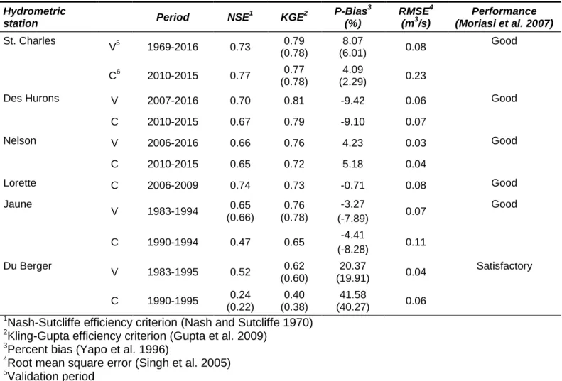
The calibration performance is “good” for all sub-watersheds (for parameter values, please refer to Supplementary material), except for the Du Berger sub-watershed which shows a “satisfactory” rating (Table 3). Calibration results using NSE-LOG as the objective function are presented in Supplementary material. Examination of the KGE values shows that some sub-watershed calibrations performed better than others. The best KGE for both the calibration (C) and the validation (V) periods were obtained for the Des Hurons (C: 0.79 and V: 0.81) and St. Charles (C: 0.77, V: 0.79) sub-watersheds. A closer look at the seasonal (spring: 03/21-06/20, summer: 06/21-09/20, fall: 09/21-12/20 and winter: 12/21-03/20) flow-duration curves confirmed that observed and simulated flows showed a good fit at the hydrometric station located on the Des Hurons River (Supplementary material). Indeed, except for the winter period which shows a small offset, the observed and simulated flow curves overlap.
Hydrometric
station Period NSE
1 KGE2 P-Bias 3 (%) RMSE4 (m3/s) Performance (Moriasi et al. 2007) St. Charles V5 1969-2016 0.73 0.79 (0.78) 8.07 (6.01) 0.08 Good C6 2010-2015 0.77 0.77 (0.78) 4.09 (2.29) 0.23
Des Hurons V 2007-2016 0.70 0.81 -9.42 0.06 Good
C 2010-2015 0.67 0.79 -9.10 0.07 Nelson V 2006-2016 0.66 0.76 4.23 0.03 Good C 2010-2015 0.65 0.72 5.18 0.04 Lorette C 2006-2009 0.74 0.73 -0.71 0.08 Good Jaune V 1983-1994 0.65 (0.66) 0.76 (0.78) -3.27 (-7.89) 0.07 Good C 1990-1994 0.47 0.65 -4.41 (-8.28) 0.11 Du Berger V 1983-1995 0.52 0.62 (0.60) 20.37 (19.91) 0.04 Satisfactory C 1990-1995 0.24 (0.22) 0.40 (0.38) 41.58 (40.27) 0.06 1Nash-Sutcliffe efficiency criterion (Nash and Sutcliffe 1970)
2Kling-Gupta efficiency criterion (Gupta et al. 2009) 3Percent bias (Yapo et al. 1996)
4Root mean square error (Singh et al. 2005) 5Validation period
6Calibration period
Table 3. Temporal and standard (in parentheses) calibration performance for each sub-watershed using NSE as the objective function.
Meanwhile, the lowest GOFI values were recorded for the Du Berger sub-watershed (Supplementary material) with particularly low values for the calibration period (C: 0.40, V: 0.62). While spring flows show a good fit, simulated summer flows are overestimated, especially for flows smaller than 5 m3/s. Fall simulated flows are greater than observed flows for values lower than 5 m3/s, except for flows smaller than 1 m3/s which are consistent with observed flows. Winter flows show reverse trends for different flow ranges. While the model underestimates flows at the hydrometric station between 0.5 m3/s and 1.3 m3/s, flows under 0.3 m3/s or between 1.3 m3/s and 2.5 m3/s are overestimated. Similar results were obtained with the calibration using NSE-LOG. These results will be further discussed later in this paper as urban storm water management is thought to have played a governing role.
The comparison between the GOFIs characterizing the multi-temporal and standard calibration (Table 3) does not reflect a systematic gain in calibration performance when using the multi-temporal calibration method, except for the P-Bias at the Jaune River hydrometric station, which shows larger
absolute values with the standard calibration method (C: -8.28% V: -7.89%) than with the multi-temporal calibration (C: -4.41%, V: -3.27%).
3.2 Stream flow analyses
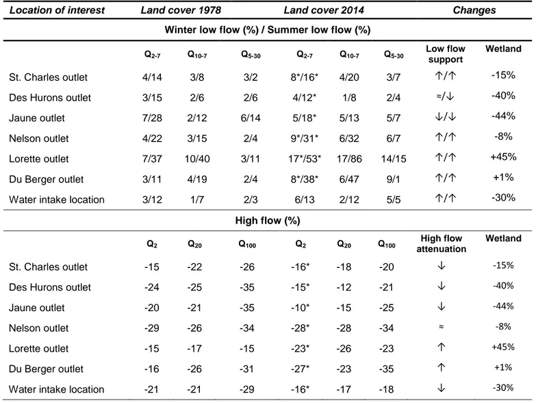
At the watershed scale, results show that winter low flow support provided by wetlands was increased from 3-4% to 3-8% given the 1978 and 2014 land cover scenarios, respectively, while summer low flows were increased from 2-14% to 7-20% during the same period (Table 4, top; for absolute values, please refer to Supplementary material). On the other hand, high flow attenuation was reduced from 15-26% for the 1978 land cover scenario to 16-20% for the 2014 scenario (Table 4, bottom). These results reflect some discrepancies in the relation between wetland change and hydrological services (section 4.2).
In contrast, at the sub-watershed scale, most of them are associated to a positive correlation between wetland change and stream flow mitigation. The Wilcoxon rank sum test (p < 0.05), used to test equality of medians, revealed that the decrease in summer low flow support was significant for the Des Hurons and the Jaune sub-watersheds. The increase in low flow support was also significant for the Nelson, Lorette, Du Berger and St. Charles sub-watersheds. The decrease or increase in high flow attenuation was also significant for all sub-watersheds, except at the Nelson outlet.
For example, results of the sub-watershed analysis of wetland changes (Table 2) showed that the Jaune River watershed had the most important relative decrease in wetland areas among sub-watersheds (-44%). The relative contribution of wetlands to low flow support for the winter period between pairs of simulations; that is for Q2-7 (2-year minimum flow over 7 days) and Q5-30 (5-year minimum flow over 30 days) decreased from 7% to 5% and 6% to 5%, respectively (Table 4, top), while it increased from 2% to 5% for Q10-7 (10-year minimum flow over 7 days). Meanwhile, for the summer period (Table 4, top), the reductions in the contribution of wetlands to low flows were more substantial, as anticipated. As illustrated in Fig. 3 (for other locations of interest, please refer to Supplementary material), the distances between the curves of paired simulations are smaller for the 2014 land cover than for the 1978 scenario, confirming that low flow support and high flow attenuation were greater in the 1978 scenario, for this sub-watershed. Wetlands in the 1978 scenario increased the summer Q2-7 by 28% (+0.12 m3/s) while those of the 2014 land cover increased by 18% (+0.08 m3/s) in 2014. Moreover, the Q5-30 decreased from 14% to 7%, while the Q10-7 remained stable, with a slight increase from 12% at 13%. On the other hand, the differences between high flow indicators between pairs of simulations also decreased from 20% to 10%, 21% to 15% and 35% to 25%, for Q2 (2-year maximum flow), Q20 (20-year maximum flow), Q100 (100-year maximum flow), respectively (Table 4, bottom).
The hydrographs at the outlet of the Jaune River sub-watershed for the Q20 event associated with the spring 2008 conditions show that the peak flow reduction was larger for the 1978 land cover scenario than for the 2014 scenario (Fig. 4). While wetlands of the 1978 land cover scenario decreased the Q20 peak flow (April 29, 2008) from 30.1 m3/s to 22.2 m3/s, the wetlands of the 2014 scenario were associated with a decrease from 31.8 m3/s to 26.9 m3/s for the same date. Additionally, the simulated hydrograph with wetlands shows a shift of the curve to the right, reflecting a lag in the peak flow timing. When comparing the paired simulations, it is also noteworthy that the recession limb reaches a larger low flow for the simulation with wetlands than that without wetlands.
Location of interest Land cover 1978 Land cover 2014 Changes
Winter low flow (%) / Summer low flow (%)
Q2-7 Q10-7 Q5-30 Q2-7 Q10-7 Q5-30 Low flow
support
Wetland
St. Charles outlet 4/14 3/8 3/2 8*/16* 4/20 3/7 ↑/↑ -15%
Des Hurons outlet 3/15 2/6 2/6 4/12* 1/8 2/4 ≈/↓ -40%
Jaune outlet 7/28 2/12 6/14 5/18* 5/13 5/7 ↓/↓ -44%
Nelson outlet 4/22 3/15 2/4 9*/31* 6/32 6/7 ↑/↑ -8%
Lorette outlet 7/37 10/40 3/11 17*/53* 17/86 14/15 ↑/↑ +45%
Du Berger outlet 3/11 4/19 2/4 8*/38* 6/47 9/1 ↑/↑ +1%
Water intake location 3/12 1/7 2/3 6/13 2/12 5/5 ↑/↑ -30%
High flow (%)
Q2 Q20 Q100 Q2 Q20 Q100 High flow
attenuation
Wetland
St. Charles outlet -15 -22 -26 -16* -18 -20 ↓ -15%
Des Hurons outlet -24 -25 -35 -15* -12 -21 ↓ -40%
Jaune outlet -20 -21 -35 -10* -15 -25 ↓ -44%
Nelson outlet -29 -26 -34 -28* -28 -34 ≈ -8%
Lorette outlet -15 -17 -15 -23* -26 -23 ↑ +45%
Du Berger outlet -16 -26 -31 -27* -23 -35 ↑ +1%
Water intake location -21 -21 -29 -16* -17 -18 ↓ -30%
Table 4. Impact of wetlands (%) on winter/summer (top) low flow support with respect to the following flow indicators: Q2-7, Q10-7 and Q5-30. Impact of wetlands (%) on high flow attenuation (bottom)
with respect to the following flow indicators: Q2, Q20 and Q100. The last column introduces the
changes in wetland area between 1978 and 2014. The asterisk refers to a significant difference between the change in the Q2-7 or Q2 given the 1978 and 2014 land cover scenarios.
Fig. 3. Flow-duration curves of annual 7-day (black lines) summer low flows and annual high flows (blue lines) at the outlet of the Jaune River sub-watershed for the land cover scenarios of 1978 (left) and 2014 (right). The 2-, 10-, 20-, and 100-year return periods are shown as dots.
Fig. 4. Impact of wetlands on the Q20 event of spring 2008, at the outlet of the Jaune River sub-watershed
4. Discussion
4.1 Calibration of the urbanized sub-watershed
The calibration performance of the Du Berger sub-watershed highlights the challenges facing hydrological modelling in urbanized watersheds (Salvadore et al., 2015). The lower values obtained for the Du Berger sub-watershed may be due to the important urban land cover (45%), where the surface routing of water from rainfall to runoff is not driven by the same processes as in the other land cover. Urbanization affects the hydrological cycle of a watershed by decreasing evapotranspiration and infiltration and increasing surface runoff. Moreover, through excavation and leveling, urban development can modify the topography and affect the natural surface drainage network of a watershed. In urbanized watersheds, the routing of water is rather controlled by urban drainage systems and storm water management practices (St-Hilaire et al., 2015). Unfortunately, at this point, urban drainage systems are not accounted for explicitly in the current computational modules of HYDROTEL. This is reflected by the positive P-Bias, which implies that the simulated flows are larger than the observed flows. This is due to the current urban drainage system implemented in Quebec City which controls combined sewer overflows using underground reservoirs and routes most of the storm runoff to a wastewater treatment plant located beyond the sub-watershed boundary (Pleau et al., 2005; Fradet et al., 2011). In order to increase the calibration performance for urbanized sub-watersheds, future work will focus on integrating the main conduits of the urban drainage system in the model. 4.2 Contrasting hydrological services with wetland change
In the St. Charles River watershed, the impact on low flow support and high flow attenuation for 1978 and 2014 land cover scenarios can be compared with the changes in the area occupied by wetlands at the sub-watershed scale (Table 4). For most sub-watersheds, the impact of wetlands on high flow attenuation was positively correlated with the changes in wetlands areas. The Lorette sub-watershed, which is known for recent flooding in 2005 and 2013 in the downstream urbanized area (City of Québec, 2017), would particularly benefit from an increase in wetland areas, in the upstream part. For low flow support in the Des Hurons, Jaune, Lorette and Du Berger River sub-watersheds, a decrease in wetland areas is associated with a decrease in low flow support, whereas an increase in wetland areas is reflected by an increase in low flow support. However, considering low flow support, two sub-watersheds present reverse tendencies, namely those of the St. Charles and the Nelson Rivers, where the decrease in wetland areas was associated with a significant increase in low flow support.
To explain these reverse tendencies, a few hypotheses would need to be tested. For example, land cover changes in the drainage areas of wetlands (e.g.: increase in impervious surfaces) should be
further investigated using archived aerial photographs. With respect to the St. Charles River outlet, the wetland areas underwent a decrease from 12.5% to 10.6% of the watershed area. However, this net decrease could be divided in: (i) losses in some parts of the watershed, and (ii) small gains in other locations (Supplementary material) that are strategically important for river flow routing, which could explain why an increase in their drainage areas was observed. This also suggests that the loss of wetlands could have modified locally the surface routing of water. Moreover, the St. Charles and Nelson sub-watersheds have been characterized by an important increase in urban areas according to the 1978 and 2014 land cover scenarios, from 5% to 16% and from 34% to 56%, respectively (Blanchette et al., 2018). Since HYDROTEL does not take into account urban drainage, results for these sub-watersheds should be taken with care. The second hypothesis to be tested refers to the small absolute flow indicator values for the two pairs of simulations (Supplementary material), which could lead to an exaggerated relative impact of wetlands. This could also explain why the reverse tendencies are observed more frequently for low flows. For example, for the 1978 land cover scenario at the Nelson River outlet where the wetland areas decreased from 19% to 18%, the Q10-7 was 0.28 m3/s with the contribution of wetlands and 0.25 m3/s without, which represents an increase of the low flow indicator of 0.03 m3/s with the contribution of wetlands. For the 2014 land cover scenario, the same low flow indicator had values of 0.30 m3/s and 0.25 m3/s, with and without the contribution of wetlands, respectively, an increase of 0.05 m3/s. As a result, the increase associated with the 1978 and 2014 land cover scenarios can be considered as negligible. Another element that could explain reverse tendencies is related to the concept of equifinality in the calibration process. The DDS algorithm leads to multiple solutions for an optimized value of the objective function. In our case, two sets of calibrated parameters were retained among other possible outputs for the NSE and the NSE-LOG. These parameters may have an impact on the simulated processes and consequently, on the simulated flows (Foulon and Rousseau, 2018a).
The effect of wetland changes on stream flows is comparable with results from other recent temperate-climate watershed studies. Evenson et al. (2018), used SWAT to assess the impact of various scenarios on storage, connectivity and stream flows, in the Pipestrem River watershed, located in the Prairie Pothole Region, in North Dakota. Their results demonstrated that the loss of depressionnal (i.e. generally isolated) wetlands resulted in increased peak flows. In contrast, they also mentioned that, using their 100% loss scenario, depressionnal wetlands did not have a sizable impact on base flow. Still using improved wetlands modules in SWAT, Lee et al. (2018) showed that the loss of geographically isolated wetlands in an agricultural watershed located within the Coastal Plain of the Chesapeake Bay Watershed decreased low flows and increased high flows. Moreover, they compared different loss
scenarios and found that the scenario showing the larger loss had a stronger impact on downstream flows.
4.3 Implications for management
A decrease in water availability represents a primary concern in the St. Charles River watershed. Indeed, the drainage area of the water intake located 11 km downstream the Lake St. Charles outlet acts as a source water watershed for more than 300,000 citizens and supply may be insufficient during low flows even in the near future (Foulon and Rousseau, 2018b). Other impacts of more severe low flows on hydrological systems include increased concentration of contaminants, temperatures, and sediments, resulting in changes to river morphology (Heicher, 1993). These physical changes, in turn, can impact aquatic habitat, by affecting the distribution and abundance of algae, vegetation, macroinvertebrates and fish (Heicher, 1993). In contrast, impacts of increased high flows on hydrological systems range from geomorphological changes, such as accelerated erosion or stream down-cutting, loss of biological integrity, decrease in water quality associated with elevated sediment transport, and flooding, resulting in damages to property and infrastructure (Acreman and Holden, 2013; Evenson et al., 2018).
In the St. Charles watershed, the contrasted findings between the different sub-watersheds show that some are more vulnerable to changes in wetland area, namely the Jaune and Lorette River sub-watersheds. From a wider perspective, this highlights the capacity of hydrological models to assist wetland management through the assessment of conservation programs focusing on hydrological services, such as legislation or creation of conservation networks (Erwin, 2009) or restoration (plugging drains, diking, controlling exotic/invasive vegetation; Erwin, 2009; Zedler and Kercher, 2005). As a tool to investigate the impacts of landscape attributes on watershed hydrology, models allow for the evaluation of physical processes at the sub-watershed level. Such assessment can be done at finer scales and this increased knowledge becomes particularly valuable to assist land managers in identifying the spatial location of the most hydrologically important wetlands in a given watershed. For instance, hydrological models are particularly adapted to identify and validate the pertinence of a given conservation network of wetlands. They could be used to assist governmental and municipal agencies in the application of the three steps of a mitigation sequence, that is: avoid, minimize and compensate. As illustrated by Fossey and Rousseau (2016b), the use of such models could highlight the benefits of using wetlands as mitigation measures of future extreme flows.
The scope of this paper was to quantitatively assess whether the changes in wetland surface area within the St. Charles River watershed between 1978 and 2014 were reflected on low flow support and high flow attenuation. The PHYSITEL/HYDROTEL modelling platform revealed that changes in wetland cover have had an effect on the capacity of the St. Charles River watershed to support low flows and attenuate high flows. For some locations of interest, the loss of wetlands was accompanied by a significant reduction in both hydrological services, while for others, an increase in wetland areas induced an increase in hydrological services. Unexpectedly, for low flow indicators, some locations of interest show a reverse tendency, that is for the outlets of the St. Charles and Nelson Rivers. These reverse tendencies could be explained by the hydrologically important increase in impervious surfaces in the drainage areas of wetlands and by the absolute values of low flow indicators. These hypotheses should be investigated in a future study using archived aerial photographs.
This paper also presented a novel approach that was introduced as a multi-temporal calibration strategy, taking advantage of the multiple land cover scenarios available for this project. The resulting GOFIs were associated with good to satisfactory calibration performances, with a slight gain in performance compared to a standard calibration.
The conclusions of this paper lead to new questions on the evolution of the studied hydrological services provided by wetlands. The methodological scheme developed in this study could also be adapted to evaluate the effect of using invariant wetland cover, to highlight the impact of urbanization or other hydrologically relevant land cover changes on the hydrological services provided by wetlands. Future modelling work should focus on identifying groups of wetlands to be protected to ensure basic hydrological services. The groups could be defined in terms of spatial attributes such as location and drainage area. Model improvements could also include the explicit accounting for the urban drainage network in the modelling platform in order to increase the ability of HYDROTEL to reproduce observed flows and assess the role of wetlands in urbanized watersheds. The potential for pursuing additional studies is promising and it is clear that increasing our understanding of the hydrological services provided by wetlands would be beneficial to municipal land planning; that is what we plan on doing next.
Acknowledgments
The authors would like to thank the City of Québec for providing precipitation data and hydrometric data for the Lorette River sub-watershed and the reviewers for their useful comments.
Funding
This work was supported by the Natural Sciences and Engineering Research Council (NSERC) of Canada through the Discovery Grant Program (A.N. Rousseau, principal investigator).
References
Acreman, M., Holden, J., 2013. How Wetlands Affect Floods. Wetlands. 5, 773-786. https://doi.org/10.1007/s13157-013-0473-2
APEL, 2015. Intoduction to issues related to the drinking water reservoir of the St. Charles Lake. p. 14 [In French].
Blanchette, M., Rousseau, A.N., Poulin, M., 2018. Mapping wetlands and land cover change with Landsat archives : the added value of geomorphologic data. Can. J. Remote Sens. https://doi.org/10.1080/07038992.2018.1525531
Blann, K.L., Anderson, J.L., Sands, G.R., Vondracek, B. 2009. Effects of Agricultural Drainage on Aquatic Ecosystems: A Review. Crit. Rev. Env. Sci. Tec. 11. 909-1001. https://doi.org/10.1080/10643380801977966
Bouda, M., Rousseau, A.N., Gumiere, S.J., Gagnon, P., Konan, B., Moussa, R., 2014. Implementation of an automatic calibration procedure for HYDROTEL based on prior OAT sensitivity and complementary identifiability analysis. Hydrol. Process. 12, 3947-3961. https://doi.org/10.1002/hyp.9882
Bouda, M., Rousseau, A.N., Konan, B., Gagnon, P., Gumiere, S.J., 2012. Bayesian uncertainty analysis of the distributed hydrological model HYDROTEL. J. Hydrol. Eng. 9, 1021-1032. https://doi.org/10.1061/(Asce)He.1943-5584.0000550
Brinson, M.M., Malvarez, A.I., 2002. Temperate freshwater wetlands: types, status, and threats. Environ. Conserv. 2, 115-133. https://doi.org/10.1017/S0376892902000085
Bullock, A., Acreman, M., 2003. The role of wetlands in the hydrological cycle. Hydrol. Earth Syst. Sc. 3, 358-389. https://doi.org/10.5194/hess-7-358-2003
City of Québec, 2017. City of Québec - Floods – Anti-flood wall on Lorette River. https://www.ville.quebec.qc.ca/citoyens/propriete/riviere_lorette.aspx (accessed November 27, 2017) [In French].
Davidson, N.C., 2014. How much wetland has the world lost? Long-term and recent trends in global wetland area. Mar. Freshwater Res. 10, 934-941. https://doi.org/10.1071/mf14173
DeFries, R., Eshleman, K.N., 2004. Land-use change and hydrologic processes: a major focus for the future. Hydrol. Process. 11, 2183-2186. https://doi.org/10.1002/hyp.5584
Diem, J.E., Hill, T.C., Milligan, R.A., 2018. Diverse multi-decadal changes in streamflow within a rapidly urbanizing region. J. Hydrol. 556, 61-71. https://doi.org/10.1016/j.jhydrol.2017.10.026
Erwin, K.L. 2009. Wetlands and global climate change : the role of wetland restoration in a changing world. Wetl. Ecol. Manag., 17 71-84
Evenson, G.R., Golden, H.E., Lane, C.R., McLaughlin, D.L., D’amico, E., 2018. Depressional wetlands affect watershed hydrological, biogeochemical, and ecological functions. Ecol. Appl. 4, 953-966. Fortin, J.-P., Turcotte, R., Massicotte, S., Moussa, R., Fitzback, J., Villeneuve, J.-P., 2001. Distributed
Watershed Model Compatible with Remote Sensing and GIS Data. I: Description of Model." J. Hydrol. Eng. 2, 91-99. https://doi.org/10.1061/(asce)1084-0699(2001)6:2(91)
Fossey, M., Rousseau, A.N., 2016a. Assessing the long-term hydrological services provided by wetlands under changing climate conditions: A case study approach of a Canadian watershed. J. Hydrol. 541 (Pt B), 1287-1302. https://doi.org/10.1016/j.jhydrol.2016.08.032
Fossey, M., Rousseau, A.N., 2016b. Can isolated and riparian wetlands mitigate the impact of climate change on watershed hydrology? A case study approach. J. Environ. Manage. 184 (Pt 2), 327-339. https://doi.org/10.1016/j.jenvman.2016.09.043
Fossey, M., Rousseau, A.N., Bensalma, F., Savary, S., Royer, A., 2015. Integrating isolated and riparian wetland modules in the PHYSITEL/HYDROTEL modelling platform: model performance and diagnosis. Hydrol. Process. 22, 4683-4702. https://doi.org/10.1002/hyp.10534
Fossey, M., Rousseau, A.N., Savary, S., 2016. Assessment of the impact of spatio-temporal attributes of wetlands on stream flows using a hydrological modelling framework: a theoretical case study of a watershed under temperate climatic conditions. Hydrol. Process. 11, 1768-1781. https://doi.org/10.1002/hyp.10750
Foufoula-Georgiou, E.Z., Takbiri, Z., Czuba, J.A., Schwenk, J., 2015. The change of nature and the nature of change in agriculture landscapes: Hydrologic regime shifts modulate ecological transitions. Water Resour. Res. 8, 6649-6671. https://doi.org/10.1002/2015WR017637
Foulon, E., Rousseau, A.N., 2018a. Equifinality and automatic calibration: What is the impact of hypothesizing an optimal parameter set on modelled hydrological processes? Can. Water Resour. J. 1, 47-67. https://doi.org/10.1080/07011784.2018.1430620
Foulon, E., Rousseau, A.N., 2018b. Surface water quantity for drinking water during low flows – sensitivity assessment solely from climate data. Water Resour. Manag. https://doi.org/10.1007/s11269-018-2107-1
Fradet, O., Pleau, M., Marcoux, C., 2011. Reducing CSOs and giving the river back to the public: innovative combined sewer overflow control and riverbanks restoration of the St. Charles River in Quebec City. Water Sci. Technol. 63 (2), 331-338. https://doi.org/10.2166/wst.2011.059 Gupta, H.V., Kling, H., Yilmaz, K.K., Martinez, G.F., 2009. Decomposition of the mean squared error
and NSE performance criteria: Implications for improving hydrological modelling. J. Hydrol. 377 (1-2), 80-91. https://doi.org/10.1016/j.jhydrol.2009.08.003
Heicher, D.W., 1993. Instream flow needs: biological literature review. Susquehanna River Basin Commission Publication No. 149, p. 37.
Lee, S., Yeo, I.-Y., Lang, M.W., Sadeghi, A.M., McCarty, G.W., Moglen, G.E., Evenson, G.R., 2018. Assessing the cumulative impacts of geographically isolated wetlands on watershed hydrology using the SWAT model coupled with improved wetland modules. J. Environ. Manage. 223, 37-48. https://doi.org/10.1016/j.jenvman.2018.06.006
Liu, Y., Yang, W., Wang, X., 2008. Development of a SWAT extension module to simulate riparian wetland hydrologic processes at a watershed scale. Hydrol. Process. 16, 2901-2915. https://doi.org/10.1002/hyp.6874
Liu,Y., Yang, W., Shao, H., Yu, Z., Lindsay, J., 2018. Development of an Integrated Modelling System for Evaluating Water Quantity and Quality Effects of Individual Wetlands in an Agricultural Watershed. Water. 6, 1-18
Magiligan, F.J., Nislow, K.H., 2005. Changes in hydrologic regime by dams. Geomorphology. (71) 1-2. 61-78. https://doi.org/10.1016/j.geomorph.2004.08.017
Ministry of Sustainable Development, the Environment and the Fight Against Climate Change, 2017. Daily hydrometric data at station 050904. Available at : http://www.cehq.gouv.qc.ca/depot/historique_donnees/fichier/050904_Q.txt (accessed August 7, 2018) [In French].
Moriasi, D.N., Arnold, J.G., Van Liew, M.W., Bingner, R.L., Harmel, R.D., Veith, T.L., 2007. Model Evaluation Guidelines for Systematic Quantification of Accuracy in Watershed Simulations. T. ASABE. 3, 885-900. https://doi.org/10.13031/2013.23153
Muma, M., Gumiere, S.J., Rousseau, A.N., 2016. Assessment of the impact of subsurface agricultural drainage on soil water storage and flows of a small watershed. Water. 8, 1-21. https://doi.org/10.3390/w8080326
Nash, J.E., Sutcliffe, J.V., 1970. River flow forecasting through conceptual models part I — A discussion of principles. J. Hydrol. 10 (3), 282-290. https://doi.org/10.1016/0022-1694(70)90255-6
Natural Resources Canada, 2013. Digital elevation model of Canada.
Noël, P., Rousseau, A.N., Paniconi, C., Nadeau, D.F., 2014. Algorithm for Delineating and Extracting Hillslopes and Hillslope Width Functions from Gridded Elevation Data. J. Hydrol. Eng. 2, 366-374. https://doi.org/10.1061/(Asce)He.1943-5584.0000783
Orlandini, S., Moretti, G., Franchini, M., Aldighieri, B., Testa, B., 2003. Path-based methods for the determination of nondispersive drainage directions in grid-based digital elevation models. Water Resour. Res. 6 https://doi.org/10.1029/2002WR001639
Pleau, M., Colas, H., Lavallée, P., Pelletier, G., Bonin, R., 2005. Global optimal real-time control of the Quebec urban drainage system. Environ. Modell. Softw. 4, 401-413. https://doi.org/10.1016/j.envsoft.2004.02.009
Ramsar Convention on Wetlands, 2018. Global Wetland Outlook: State of the World’s Wetlands and their Services to People. Ramsar Convention Secretariat. Gland, Switzerland. 88 p.
Rawls, W.J., Brakensiek, D.L., 1989. Estimation of soil water retention and hydraulic properties, in: Morel-Seytoux, H.J. (Ed.), Unsaturated Flow in Hydrologic Modeling: Theory and practice. Springer Netherlands, pp. 275-300.
Roche, M. F., 1986. Dictionary of Surface Water Hydrology. Masson. 288 p. [In French]
Rousseau, A. N., Fortin, J.-P., Turcotte, R., Royer, A., Savary, S., Quévy, F., Noël, P., Paniconi, C., 2011. PHYSITEL, a specialized GIS for supporting the implementation of distributed hydrological models. Water News Off. Mag. Can. Water Resour. Assoc. 1, 18-20.
Salvadore, E., Bronders, J., Batelaan, O., 2015. Hydrological modelling of urbanized catchments: A
review and future directions. J. Hydrol. 529 (Pt 1), 62-81.
https://doi.org/10.1016/j.jhydrol.2015.06.028
Savary, S., Rousseau, A.N., Quilbe, R., 2009. Assessing the Effects of Historical Land Cover Changes on Runoff and Low Flows Using Remote Sensing and Hydrological Modeling. J. Hydrol. Eng. 6, 575-587. https://doi.org/10.1061/(Asce)He.1943-5584.0000024
Singh, J., Knapp, H.V., Arnold, J.G., Demissie, M., 2005. Hydrologic modeling of the Iroquois river watershed using HSPF and SWAT. J. Am. Water Resour. As. 2, 343-360. https://doi.org/10.1111/j.1752-1688.2005.tb03740.x
Soil Landscapes of Canada Working Group, 2010. Soil Landscapes of Canada, v3.2.
St-Hilaire, A., Duchesne, S., Rousseau, A.N., 2015. Floods and water quality in Canada: A review of the interactions with urbanization, agriculture and forestry. Can. Water Resour. J. 1-2, 273-287. https://doi.org/10.1080/07011784.2015.1010181
Tolson, B.A., Shoemaker, C.A., 2007. Dynamically dimensioned search algorithm for computationally efficient watershed model calibration. Water Resour. Res. 1, 1-16. https://doi.org/10.1029/2005WR004723
Turcotte, R., Fortin, J.-P., Rousseau, A.N., Massicotte, S., Villeneuve, J.-P., 2001. Determination of the drainage structure of a watershed using a digital elevation model and a digital river and lake network. J. Hydrol. 240 (3-4), 225-242. https://doi.org/10.1016/S0022-1694(00)00342-5
Turcotte, R., Fortin, L.-G., Fortin, V., Fortin, J.-P., Villeneuve, J.-P., 2007. Operational analysis of the spatial distribution and the temporal evolution of the snowpack water equivalent in southern Québec, Canada. Hydrol. Res. 3, 211-234. https://doi.org/10.2166/nh.2007.009
Turcotte, R., Rousseau, A.N., Fortin, J.-P., Villeneuve, J.-P., 2003. A Process-Oriented, Multiple-Objective Calibration Strategy Accounting for Model Structure, in: Duan, Q., Gupta, H.V., Sorooshian, S., Rousseau, A.N., Turcotte, R. (Eds.), Calibration of Watershed Models, American Geophysical Union, Washington, pp. 153-163.
Wang, X., Shang, S., Qu, Z., Liu, T., Melesse, A.M., Yang, W., 2010. Simulated wetland conservation-restoration effects on water quantity and quality at watershed scale. J. Environ. Manag. 91 (7), 1511-1525. https://doi.org/10.1016/j.jenvman.2010.02.023
Wang, X., Yang, W., Melesse, A.M., 2008. Using Hydrologic Equivalent Wetland Concept Within SWAT to Estimate Streamflow in Watersheds with Numerous Wetlands. T. ASABE. 1, 55-72. https://doi.org/10.13031/2013.24227
Watson, K.B., Ricketts, T., Galford, G., Polasky, S., O'Niel-Dunne, J., 2016. Quantifying flood mitigation services: The economic value of Otter Creek wetlands and floodplains to Middlebury, VT. Ecol. Econ. 130, 16-24. https://doi.org/10.1016/j.ecolecon.2016.05.015
Wilcoxon, F., 1945. Individual Comparisons by Ranking Methods. Biometrics Bull. 6, 80-83. https://doi.org/10.2307/3001968
Wu, K., Johnston, C.A., 2008. Hydrologic comparison between a forested and a wetland/lake
dominated watershed using SWAT. Hydrol. Process. 10, 1431-1442.
https://doi.org/10.1002/hyp.6695
Yapo, P.O., Gupta, H.V., Sorooshian, S., 1996. Automatic calibration of conceptual rainfall-runoff models: sensitivity to calibration data. J. Hydrol. 181 (1-4), 23-48. https://doi.org/10.1016/0022-1694(95)02918-4
Zedler, J.B., Kercher, S., 2005. Wetland resources: Status, Trends, Ecosystem Services, and
Restorability. Annu. Rev. Env. Resour. 1, 39-74.
Supplementary material
Abbreviation Definition Abbreviation Definition
C Calibration Q10-7 10-year minimum flow over 7 days
DEM Digital elevation model Q5-30 5-year minimum flow over 30 days DDS Dynamically dimensioned search
algorithm Q2 2-year maximum flow
GIS Geographic information system Q20 20-year maximum flow GOFI Goodness-of-fit indicator Q100 100-year maximum flow
HEW Hydrologically equivalent wetland RHHU Relatively homogeneous hydrological units
KGE Kling-Gupta efficiency criterion RMSE Root mean square error
NSE Nash-Sutcliffe efficiency criterion SWAT Soil and Water Assessment Tool NSE-LOG NSE calculated on logarithmic flows SWIM Soil and Water Integrated Model
P-bias Percent bias V Validation
Q2-7 2-year minimum flow over 7 days Table1. List of abbreviations.
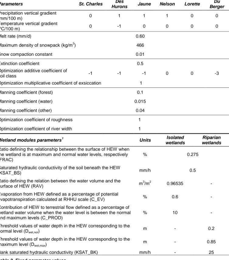
Parameters St. Charles Des
Hurons Jaune Nelson Lorette
Du Berger Precipitation vertical gradient
(mm/100 m) 0 1 1 1 0 0
Temperature vertical gradient
(°C/100 m) 0 -1 0 0 0 0
Melt rate (mm/d) 0.60
Maximum density of snowpack (kg/m3) 466
Snow compaction constant 0.01
Extinction coefficient 0.5
Optimization additive coefficient of
soil class -1 -1 -1 0 0 -3
Optimization multiplicative coefficient of exsiccation 1
Manning coefficient (forest) 0.1
Manning coefficient (water) 0.015
Manning coefficient (other) 0.04
Optimization coefficient of roughness 1 Optimization coefficient of river width 1
Wetland modules parameters1 Units Isolated
wetlands
Riparian wetlands Ratio defining the relationship between the surface of HEW when
the wetland is at maximum and normal water levels, respectively (FRAC)
% 0.275
Saturated hydraulic conductivity of the soil beneath the HEW
(KSAT_BS) mm/h 0.5
Ratio defining the relation between the water volume and the
surface of HEW (RAV) m
3
/m2 0.96535 -
Evaporation from HEW defined as a percentage of potential
evapotranspiration calculated at RHHU scale (C_EV) % 0.6 -
Contribution of HEW to terrestrial flow defined as a percentage of wetland water volume when the water level is between the normal and maximum levels (C_PROD)
% 10 -
Threshold values of water depth in the HEW corresponding to the
normal level (Dwet,nor) m - 0.2
Threshold values of water depth in the HEW corresponding to the
maximum level (Dwet,max) m - 0.85
Bank saturated hydraulic conductivity (KSAT_BK) mm/h - 25
Table 2. Fixed parameter values.
1
The selection of the parameter values associated with the wetland modules was done with due consideration of the dominant wetland typology, that is forested wetlands (swamps and forested peatlands).
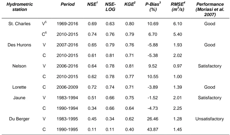
Hydrometric station
Period NSE1 NSE-LOG KGE2 P-Bias3 (%) RMSE4 (m3/s) Performance (Moriasi et al. 2007) St. Charles V5 1969-2016 0.69 0.63 0.80 10.69 6.10 Good C6 2010-2015 0.74 0.76 0.79 6.70 5.40
Des Hurons V 2007-2016 0.65 0.79 0.76 -5.88 1.93 Good C 2010-2015 0.61 0.81 0.71 -5.38 2.02 Nelson V 2006-2016 0.64 0.78 0.81 9.52 0.97 Satisfactory C 2010-2015 0.62 0.78 0.77 10.55 1.00 Lorette C 2006-2009 0.72 0.74 0.71 -3.89 1.39 Good Jaune V 1983-1994 0.51 0.66 0.75 -1.52 2.01 Satisfactory C 1990-1994 0.34 0.66 0.64 -4.73 2.25 Du Berger V 1983-1995 0.45 0.34 0.62 26.46 1.28 Unsatisfactory C 1990-1995 0.11 0.11 0.40 43.87 1.45
1Nash-Sutcliffe efficiency criterion (Nash and Sutcliffe 1970) 2Kling-Gupta efficiency criterion (Gupta et al. 2009)
3Percent bias (Yapo et al. 1996)
4Root mean square error (Singh et al. 2005) 5Validation period
6Calibration period
Table 3. Temporal calibration performance for each sub-watershed using NSE-LOG as the objective function.
Fig. 3. Seasonal flow-duration curves at the hydrometric station located on the Des Hurons River for the validation period (2007-2016).
Fig. 4. Seasonal flow-duration curves at the hydrometric station located on the Du Berger River for the validation period (1983-1995).
St. Charles outlet Des Hurons outlet Jaune outlet Nelson outlet Lorette outlet Du Berger outlet Water intake location 1978 2014 1978 2014 1978 2014 1978 2014 1978 2014 1978 2014 1978 2014 W in te r lo w fl o w s ↑ ≈ ↓ ↑ ↑ ↑ ↑ Q2 -7 W 3.24 2.85 1.02 0.99 0.37 0.35 0.44 0.44 0.28 0.25 0.51 0.36 2.17 2.12 Ø 3.10 2.65 0.99 0.95 0.35 0.34 0.42 0.40 0.26 0.22 0.50 0.33 2.12 2.00 % 4 8* 3 4 7 5 4 9* 7 17* 3 8* 3 6 Q1 0 -7 W 2.83 2.50 0.90 0.88 0.30 0.30 0.37 0.35 0.19 0.16 0.42 0.29 1.89 1.79 Ø 2.76 2.40 0.88 0.86 0.29 0.28 0.36 0.33 0.18 0.14 0.41 0.27 1.86 1.76 % 3 4 2 1 2 5 3 6 10 17 4 6 1 2 Q5 -3 0 W 3.29 2.90 0.96 0.96 0.35 0.34 0.41 0.42 0.26 0.24 0.48 0.34 2.05 2.05 Ø 3.20 2.81 0.94 0.95 0.33 0.32 0.40 0.39 0.26 0.21 0.47 0.32 2.02 1.94 % 3 3 2 2 6 5 2 6 3 14 2 9 2 5 S u m m e r l o w fl o w s ↑ ↓ ↓ ↑ ↑ ↑ ↑ Q2 -7 W 4.50 4.69 1.42 1.41 0.52 0.51 0.53 0.62 0.29 0.39 0.60 0.52 2.98 3.20 Ø 3.93 4.04 1.24 1.26 0.40 0.43 0.43 0.47 0.21 0.26 0.54 0.38 2.66 2.84 % 14 16* 15 12* 28 18* 22 31* 37 53* 11 38* 12 13* Q1 0 -7 W 3.07 3.37 0.99 1.07 0.27 0.34 0.32 0.38 0.18 0.26 0.48 0.38 1.87 2.26 Ø 2.85 2.80 0.93 0.98 0.24 0.30 0.28 0.28 0.13 0.14 0.40 0.26 1.76 2.02 % 8 20 6 8 12 13 15 32 40 86 19 47 7 12 Q5 -3 0 W 5.41 6.60 1.48 1.61 0.51 0.62 0.45 0.60 0.41 0.69 0.74 0.72 2.88 3.53 Ø 5.30 6.18 1.40 1.56 0.44 0.58 0.43 0.56 0.37 0.60 0.71 0.71 2.80 3.36 % 2 7 6 4 14 7 4 7 11 15 4 1 3 5 A n n u a l h ig h fl o w s ↓ ↓ ↓ ≈ ↑ ↑ ↓ Q2 W 72.95 80.20 27.35 30.40 12.75 14.70 8.04 8.63 16.35 15.90 6.15 8.50 41.95 47.20 Ø 85.60 95.30 36.10 35.80 15.95 16.25 11.30 12.00 19.15 20.70 7.33 11.70 53.35 56.50 % -15 -16* -24 -15* -20 -10* -29 -28* -15 -23* -16 -27* -21 -16* Q2 0 W 129.00 145.00 43.60 51.90 23.90 27.00 14.00 14.30 21.20 20.40 11.50 13.00 79.00 87.50 Ø 166.00 176.00 58.50 59.10 30.10 31.80 19.00 19.80 25.40 27.40 15.60 16.90 99.60 106.00 % -22 -18 -25 -12 -21 -15 -26 -28 -17 -26 -26 -23 -21 -17 Q1 00 W 180.00 205.00 89.60 108.00 43.10 49.50 17.80 18.10 23.50 22.40 26.60 29.30 118.00 138.00 Ø 242.00 257.00 137.00 136.00 66.10 66.00 26.90 27.60 27.80 29.20 38.70 44.90 167.00 169.00 % -26 -20 -35 -21 -35 -25 -34 -34 -15 -23 -31 -35 -29 -18
Changes in wetland area extent (%)
-15 -40 -44 -8 +45 +1 -30
Table 4. Low flow (Q2-7, Q10-7 and Q5-30) and high flow (Q2, Q20 and Q100) indicators for the
simulations with and without wetlands of the 1978 and 2014 land cover scenarios. W: simulation with wetlands, Ø: simulation without wetlands, %: percent difference between the indicator with and without the wetlands modules activated. The asterisk refers to a significant difference between the attenuation of the Q2-7 or Q2 in 1978 and
2014. The arrows represent the changes in stream flow regulation provided by wetlands.
Fig. 5. Flow-duration curves of annual 7-day (black lines) summer low flows and annual high flows (blue lines) at the outlet of the St. Charles River watershed for the land cover scenarios of 1978 (left) and 2014 (right). The 2-, 10-, 20-, and 100-year return periods are shown as dots.
Fig. 6. Flow-duration curves of annual 7-day (black lines) summer low flows and annual high flows (blue lines) at the outlet of the Du Berger River watershed for the land cover scenarios of 1978 (left) and 2014 (right). The 2-, 10-, 20-, and 100-year return periods are shown as dots.
Fig. 7. Flow-duration curves of annual 7-day (black lines) summer low flows and annual high flows (blue lines) at the water supply uptake for the land cover scenarios of 1978 (left) and 2014 (right). The 2-, 10-, 20-, and 100-year return periods are shown as dots.
Fig. 8. Flow-duration curves of annual 7-day (black lines) summer low flows and annual high flows (blue lines) at the outlet of the Nelson River sub-watershed for the land cover scenarios of 1978 (left) and 2014 (right). The 2-, 10-, 20-, and 100-year return periods are shown as dots.
Fig. 9. Flow-duration curves of annual 7-day (black lines) summer low flows and annual high flows (blue lines) at the outlet of the Des Hurons River watershed for the land cover scenarios of 1978 (left) and 2014 (right). The 2-, 10-, 20-, and 100-year return periods are shown as dots.
Fig. 10. Flow-duration curves of annual 7-day (black lines) summer low flows and annual high flows (blue lines) at the outlet of the Lorette River watershed for the land cover scenarios of 1978 (left) and 2014 (right). The 2-, 10-, 20-, and 100-year return periods are shown as dots.
Fig. 11. Examples of a) local losses and b) local gains in wetland areas and drainage areas for a net decrease from 12.5% to 10.6 % in wetland areas at the watershed scale.