Waveform inversion based on wavefield decomposition

(1)

HAL Id: tel-01299534

https://pastel.archives-ouvertes.fr/tel-01299534

Submitted on 7 Apr 2016

HAL is a multi-disciplinary open access archive for the deposit and dissemination of sci-entific research documents, whether they are pub-lished or not. The documents may come from teaching and research institutions in France or abroad, or from public or private research centers.

L’archive ouverte pluridisciplinaire HAL, est destinée au dépôt et à la diffusion de documents scientifiques de niveau recherche, publiés ou non, émanant des établissements d’enseignement et de recherche français ou étrangers, des laboratoires publics ou privés.

To cite this version:

Fang Wang. Waveform inversion based on wavefield decomposition. Geophysics [physics.geo-ph]. Ecole Nationale Supérieure des Mines de Paris, 2015. English. �NNT : 2015ENMP0043�. �tel-01299534�

(2)

MINES ParisTech Centre de Géosciences

École doctorale n° 398

Géosciences, Ressources Naturelles et Environnement

Ce

présentée et soutenue publiquement par

Fang WANG

le 16 Octobre 2015

Waveform inversion based on wavefield decomposition

L’inversion des formes d’ondes par décomposition des champs d’ondes

Doctorat ParisTech

T H È S E

pour obtenir le grade de docteur délivré par

_{l’École nationale supérieure des mines de Paris}

_{Spécialité “Dynamique et Ressources des Bassins Sédimentaires”}

Directeur de thèse : Hervé CHAURIS Co-encadrement de la thèse : Daniela DONNO

T

H

È

S

E

Jury

M. Stéphane OPERTO, Directeur de recherche, CNRS, Géoazur Président M. Paul SAVA, Professeur, Colorado School of Mines, Etats-Unis Rapporteur M. Gilles LAMBARE, Directeur de recherche, CGG, professeur associé IPGP Rapporteur M. Romain BROSSIER, Maître de conférences, Université Joseph Fourier Grenoble I Examinateur

M. Hervé CHAURIS, Professeur, MINES ParisTech Examinateur

Mme Daniela DONNO, Maître de conférences, MINES ParisTech Examinatrice

(3)

(4)

I would like to thank all the people who have contributed to this thesis work.

First of all, I would like to thank my advisers Hervé Chauris and Daniela Donno. I thank them for their availability, patience, support and encouragement given along my stay in the geophysics group. I thank them also for having trusted in my ability to develop this research even though I had not much experience in geophysics before the thesis. I especially acknowledgement their patience with me and explain to me even the basic knowledge and formulations. This really helps me to start the thesis in the irst year. The discussions with them have always been helpful for me. Thanks for their availability even on weekends to answer my questions or to help me revising reports and presentations. Their passion and persistence for the research also encourage me.

I would like to thank the members of my jury. Thanks to Paul Sava and Gilles Lambaré for having accepted to review my thesis in detail. Thanks to Stéphane Operto and Romain Brossier for examining my thesis.

I thank Total for inancially and technically supporting my thesis. I especially ac-knowledge Henri Calandra from Total who has brought me to the area of geophysics and initiated this PhD project. I thank François Audebert from Total for providing the real data set used for the real application in this thesis and for his help to apply for the com-putational resources from Total. I thank Florent Ventimiglia from Total for kindly helping me with troublesome computer and account problems.

Many thanks to the members in the geophysics team of the Geosciences Center at MINES ParisTech. I especially thank Véronique Lachasse for her help to facilitate the administrative afairs since my irst day at the oice. Thanks to the Alexandrine Gesret and Mark Noble for their availability and advices.

I would like to thank all my oicemates during the three and half years. Nidhal Be-layouni, Sébastien Penz, Carlos Pérez, Elise Vi Nu Bas, Charles-Antoine Lameloise, Em-manuel Cocher, Sven Schilke, Yves-Marie Batany, Yubing Li and Hao Jiang for their friend-ship and support. Thanks Elise for ofering me facilities when I arrived in Fontainebleau. I also thank Dominique Vassiliadis from the Geosciences Center and Evelyne Peyrillou from the delegation to help me solving administrative matters regarding the visa, contract, residence cart, etc.

Finally, I would like to thank my family for always respecting and supporting my professional and life choices. My research would not have been possible without their support. Before continuing with the text of this research, I would like to especially thank my boyfriend Haisheng Wang who voluntarily came to France to accompany me and has always been at my side and supporting me during these years.

(5)

(6)

The knowledge of the Earth subsurface poses economic, environmental, human and sci-entiic issues. Seismic imaging is a procedure to image the Earth subsurface from the data observed at the surface. In the context of hydrocarbon exploration, seismic imaging techniques are widely used to characterise the irst few kilometres of the Earth’s interior. Full Waveform Inversion (FWI) is one of the eicient seismic imaging method. Recent ad-vances in high performance computer make FWI feasible for large applications. In theory, FWI could reconstruct a high-resolution subsurface image provided that low frequency and wide angle/aperture/azimuth data are available. FWI is a data-itting procedure and is resolved as an optimization problem. Depending on the frequency content of the data, the objective function of FWI may be highly nonlinear and has many local minima. If a data set mainly contains relections, this problem particularly prevents the gradient-based methods from recovering the long wavelengths of the velocity model.

The model of the subsurface could be separated into two parts by scale separation. One part is the short-wavelength part which contains the singularities of the model and the other part is the long-wavelength part which is a smooth version of the model. In this thesis, I propose a variant of FWI based on the scale separation of these two parts to mitigate the nonlinearity of the problem.

In the irst section, methodologies of the conventional FWI and the new proposed method are presented. The new method is a Relection-based Waveform Inversion (RWI) method . It consists of decomposing the gradient of FWI into a short-wavelength part and a long-wavelength part and the inversion is performed in an alternating fashion between these two parts. The gradient decomposition is achieved by decomposing the waveields into their one-way components. Diferent waveield decomposition methods are also pre-sented.

In the second section, we implement the FWI and the new method to several case studies. For numerical modeling, we use a inite-diference approach to resolve the acoustic wave equation with constant density in the time domain. The model update is based on the L-bfgs algorithm and the waveield is decomposed using the 2D FFT-based method in the �-� domain. These case studies show the diiculties associated with FWI to recover the long-wavelength part of the velocity model when low frequency and large-ofset data are absent, and the initial model is far from the true one. The new method shows its robustness in this case especially for constructing the long-wavelength model.

(7)

(8)

La connaissance du sous-sol de la Terre pose les enjeux économiques, environnementaux, humains et scientiiques. L’imagerie sismique est une procédure à imager le sous-sol à par-tir des données observées à la surface. Dans le cadre de l’exploration des hydrocarbures, les méthodes d’imagerie sismique sont beaucoup utilisées pour caractériser les premiers kilomètres de l’intérieur de la Terre. Full Waveform Inversion (FWI) est l’une des méth-odes d’imagerie sismique eicace. Les progrès récents en superordinateur rendent FWI possible pour les grandes applications. En théorie, FWI pourrait reconstruire une image du sous-sol à haute résolution, à condition que les données de basse fréquences et grand-angle/ouverture/azimut sont disponibles. FWI est une procédure d’ajuster des données, et est résolu comme un problème d’optimisation. En fonction du contenu en fréquence des données, la fonction objectif de FWI peut être fortement non linéaire et présente de nombreux minima locaux. Pour des données qui contiennent principalement des rélex-ions, ce problème empêche notamment les méthodes basées sur le gradient de retrouver les longues longueurs d’onde du modèle de vitesse.

Le modèle du sous-sol peut être séparé en deux parties par separation d’échelle. Une partie est la partie courte longueur d’onde qui contient les singularités du modèle. l’autre partie est la partie longue longueur d’onde qui est une version lisse du modèle. Dans cette thèse, nous proposons une variante de FWI basée sur la séparation d’échelle entre les deux parties pour atténuer la non-linéarité du problème.

Dans la première section, les méthodologies de la FWI classique et la nouvelle méthode proposée sont présentés. La nouvelle méthode est une méthode de l’inversion des formes d’ondes basées sur les rélexions. Il consiste à décomposer le gradient de FWI en une partie de courte longueur d’onde et une partie de longue longueur d’onde, et l’inversion est efectuée d’une manière alternée entre ces deux parties. La décomposition du gradient est obtenu par la décomposition des champs d’ondes en leurs composants unidirectionnels. Diférentes méthodes de décomposition des champs d’ondes sont également présentées.

Dans la deuxième section, nous appliquons la FWI et la nouvelle méthode à plusieurs études de cas. Pour la modélisation numérique, nous utilisons une approche diférence inie pour résoudre l’équation des ondes acoustiques avec une densité constante dans le domaine temporel. La mise à jour du modèle est basé sur l’algorithme L-BFGS et les champs d’ondes sont décomposés en utilisant la méthode basée sur FFT 2D dans le domaine � - �. Ces études montrent les diicultés liées à FWI pour récupérer la partie longue longueur d’onde du modèle de vitesse lorsque les données de basse fréquence et grands ofsets sont absentes, et le modèle initial est loin du vrai modèle. La nouvelle méthode présente sa robustesse dans ce cas en particulier pour la construction du modèle de longue longueur d’onde.

Mots Clés: Inversion des formes d’ondes, décomposition des champs d’ondes, imagerie sismique.

(9)

(10)

List of igures

1-1 Wavenumber at a scattering point [Huang and Schuster, 2014]. . . 30 1-2 Separation of scales between the frequency content of the velocity model

and of the seismic data [Claerbout, 1982]. . . 32 2-1 An example of seismic data. We can observe the direct wave and the

re-lected waves. . . 41 2-2 The original Ricker wavelet (black) and the estimated source (red) in the

frequency domain (left) and in the time domain (right). . . 45 2-3 Wavenumber illumination. One source-receiver pair, one scattering point

and one frequency in the data provides one wavenumber in the image space [Huang and Schuster, 2014]. . . 50 2-4 Approximate resolution limits for (a) diving waves, (b) and (c)

relection-related transmission, (d) difraction-relection-related transmission and (e) relection migration [Huang and Schuster, 2014]. . . 51 2-5 First Fresnel zone for the specular relection [Huang and Schuster, 2014]. . 52 2-6 Wavepath for the irst-order free-surface multiple [Huang and Schuster, 2014]. 53 2-7 a) Ray diagram for interbed multiples generated by a difractor in a thin

layer and b) the associated mirror sources diagram [Huang and Schuster, 2014]. . . 53 2-8 1D exact velocity model. . . 54 2-9 Four Ricker wavelets. From top to bottom and from left to right, the central

frequency is respectively 4 Hz, 8 Hz, 12 Hz, and 16 Hz. . . 55 2-10 (Left) Gradient of the irst iteration of FWI with source wavelets displayed

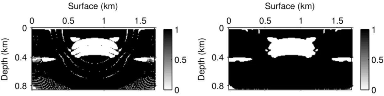
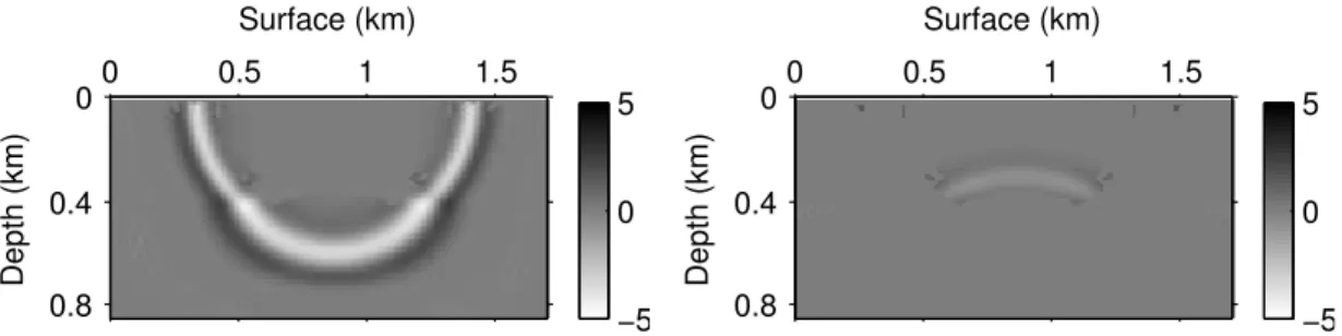
in Figure 2-9. The central frequency is respectively 4 Hz, 8 Hz, 12 Hz, and 16 Hz. (Right) The bandwidth of the vertical slice taken at the middle of each model on the left. . . 56 2-11 (Left) Gradient of the irst iteration of FWI for data with ofset range

[0–0.17] km, [0.34–0.51] km, [0.68–0.85] km respectively. (Right) The band-width of the vertical slice taken at the middle of each model on the left. . . 57 2-12 Comparison of the convergence rate of local methods applied on a 2D linear

inverse problem. The problem is solved using a) Gauss-Newton, b) gradi-ent descgradi-ent, c) preconditioned gradigradi-ent and d) conjugate-gradigradi-ent methods. The gradient in c) was preconditioned with the diagonal term of the inverse Hessian [Sirgue, 2003]. . . 60

(15)

2-13 Principle of cycle-skipping problem [Virieux and Operto, 2009]. If the phase mismatch is less than one half of the period, the local optimization methods could adjust the correct phase. In the contrary case, the local optimization methods adjust these two signals with one period shift and the inversion

falls into a local minimum. [Virieux and Operto, 2009] . . . 61

2-14 Exact velocity model. . . 61

2-15 Initial velocity model.. . . 62

2-16 Conventional FWI result.. . . 62

2-17 Velocity perturbation obtained with conventional FWI. . . 62

2-18 Multiscale FWI results. From top to bottom, the frequency used is 1.8 Hz, 2.5 Hz, 3.5 Hz, 5 Hz, 7 Hz, 10 Hz, 14 Hz respectively. For each frequency, 25 iterations of FWI is performed. . . 63

2-19 Velocity perturbation found with multiscale FWI. . . 64

3-1 Raypaths and illumination in the model space for diferent components of the gradient. Schematic wave propagation in 1D layer model. �+_{: direct} forward waveield (red solid line). �−: relected forward waveield (red dashed line). �−: direct backward waveield (blue solid line) and �+: relected backward waveield (blue dashed line). . . 69

3-2 Comparison of conventional FWI (left) and the decomposition-based wave-form inversion (right). . . 70

3-3 The initial velocity model. It is the sum of the homogeneous model at 2 km/s and the true relectivity model. The true relectivity is obtained by subtracting the smoothed true velocity model from the exact velocity model of Figure 2-8. . . 73

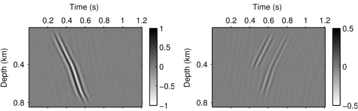
3-4 Correlation of decomposed forward and backward waveields for one source-receiver pair with the model in Figure 3-3. The source is located at 0.85 km. From top to bottom, the receivers are at 0.085 km, 0.85 km and 1.615 km respectively. Correlation of �+ _{and �}− (left); �− and �+ (right). . . . 74

3-5 Correlation of decomposed forward and backward waveields for one source-receiver pair with the model in Figure 3-3. The source is located at 0.85 km. From top to bottom, the receivers are at 0.085 km, 0.85 km and 1.615 km respectively. Correlation of �+ _{and �}+ _{(left); �}− and �− (right). . . . 75

3-6 Correlation of decomposed forward and backward waveield for the source located at 0.85 km with the model in Figure 3-3. Correlation of �+ _and �− (top left); �− and �+ (top right); �+ and �+ (bottom left); �− and �− (bottom right). . . 76

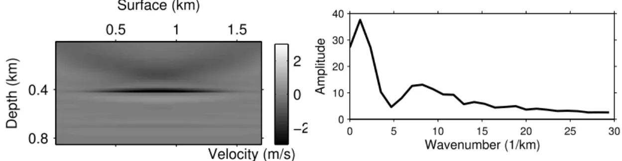
3-7 (Left) Correlation of forward waveield � and backward waveield � using all the available sources at the surface, starting from the model in Figure 3-3. (Right) Amplitude of spectrum of the vertical velocity proile taken at 0.85 km in the igure on the left.. . . 76

3-8 Correlation of decomposed forward waveield and backward waveield using all the available sources at the surface, starting from the model in Figure 3-3 (left). From top to bottom, correlation of �+ _{and �}−; �− and �+; �+ and �+_{; �}− and �− respectively. (right) Spectra of the vertical velocity proiles taken at 0.85 km for igures on the left respectively. . . 77

(16)

3-9 Direct and backpropagated waveield in the model in Figure 2-8. . . 78 3-10 Decomposed waveields for the initial waveields in Figure 3-9. �+ _(top

left), �+ _{(top right), �}− (bottom left) and �− (bottom right). . . 79

3-11 Four waveields in equation (3.11). �0_{(top left), �� (top right), �� (bottom}

left) and �0 _{(bottom right).} _{. . . 79}

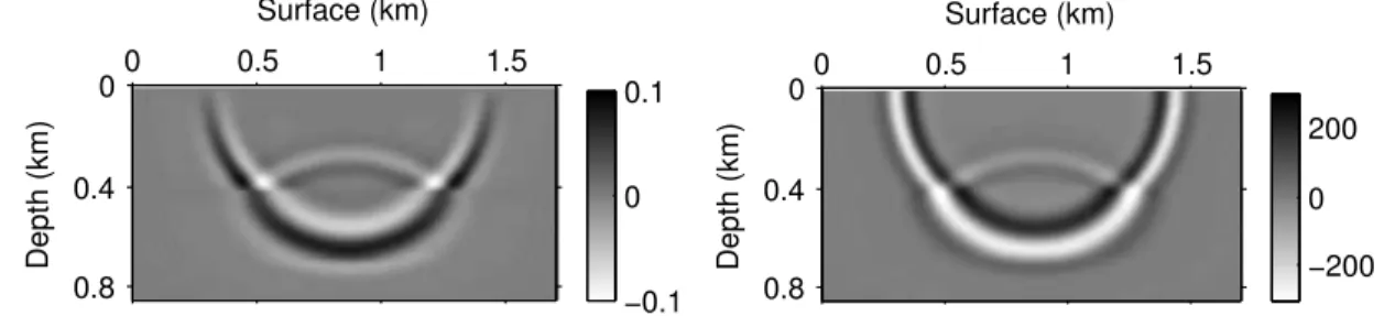
3-12 Gradients in equation (3.11). Correlation of (left) �0 _{and ��, (right) ��}

and �0_{. To be compared with Figure 3-8 (last two panels).} _{. . . 79}

3-13 One snapshot of the waveield propagated in the model in Figure 2-8 at � = 0.525 s. . . 82 3-14 (Left) The section of the waveield in the � − � domain for � = 0.85 km in

the middle of the model. (Right) FT of the igure on the left in the � − �z

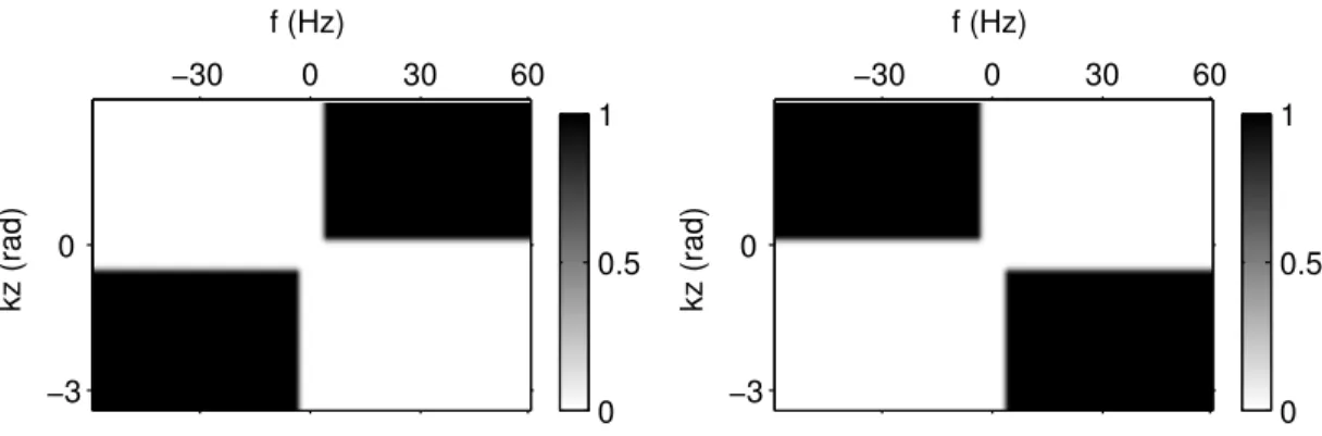
domain. . . 83 3-15 The down-going and up-going ilter in the � − �z domain. . . 83

3-16 Filtered parts of the initial image in Figure 3-14.. . . 84 3-17 Decomposed waveields in the � − � domain. Notice the diferent color-scale

between the two images. . . 84 3-18 Decomposed waveields in the space domain using the 2D FT-based

decom-position. �+ _{(left) and �}− (right). . . 84

3-19 (Left) Partial derivative of the waveield with respect to �. (Right) Partial derivative of the waveield with the respect to �. . . 86 3-20 The product of the two images in Figure 3-19. . . 86 3-21 The decomposed waveields using Poynting-vector method. �+ _{(left) and}

�− (right).. . . 87

3-22 Original mask (left) and median-iltered mask (right) for the decomposition by the Poynting-vector method. . . 87 3-23 Decomposed waveields using the mask in Figure 3-22 on the right. �+

(left) and �− (right). . . 88

3-24 A scale example of curvelet [Chauris et al., 2006]. . . 88 3-25 A direction example of curvelet [Chauris et al., 2006]. . . 88 3-26 The direction (left) and scale (right) ilter in the curvelet domain [Chauris

and Nguyen, 2008]. . . 89 3-27 Two snapshots at diferent recording time for � = 0.525 s (left) and � = 0.54

s (right). . . 89 3-28 One direction after the curvelet transform for the two snapshots in Figure 3-27. 90 3-29 Decomposed waveields using the curvelet method. �+ _{(left) and �}− (right). 91

3-30 One snapshot of the waveield propagated in the Marmousi model. . . 93 3-31 Decomposed waveields using the 2D FT method (irst panel), Poynting

method (second panel) and curvelet method (third panel). �+ _{(left) and}

�− (right).. . . 94

4-1 1D layer exact velocity model. . . 98 4-2 Final inversion results using a homogeneous initial model for FWI (irst

panel), long-wavelength model obtained with DWI (second panel), and FWI result starting from model in the second panel (third panel). Velocity pro-iles at 0.85 km (fourth panel) for the exact model (black line), initial model (red line), FWI (blue line) and DWI + FWI (green line). . . 99

(17)

4-3 2D exact velocity model [Perrone, 2013]. . . 100 4-4 Initial velocity models considered for 2D model in Figure 4-3.

Gradient-constant model (top) and homogeneous model (bottom). . . 100 4-5 Source wavelet in the time domain (left) and in the frequency domain

(right). The black lines represent the initial Ricker wavelet with central frequency of 8 Hz and the red lines represent the wavelet after the high-pass Butterworth iltering with cut frequency of 8 Hz. . . 100 4-6 Test 1. FWI result after 100 iterations. . . 101 4-7 Test 1. 1D vertical proiles of exact (black), initial (red) and FWI model

(blue). From top to bottom: � = 0.4, 1, 1.6 km. . . 102 4-8 Test 1. Top panels: shot gathers for observed data (left), initial data

(mid-dle) and inal data obtained with FWI (right). Bottom panels: observed (black), initial (red) and modeled (blue) seismic traces taken at three ofset positions: 0.5 km (top), 1.5 km (middle) and 2.5 km (bottom). Note that the observed data and the modeled data are overlapped. . . 103 4-9 Test 2. FWI result after 100 iterations. . . 103 4-10 Test 2. 1D vertical proiles of exact (black), initial (red) and FWI model

(blue). From top to bottom: � = 0.4, 1, 1.6 km. . . 104 4-11 Test 2. Top panels: shot gathers for observed data (left), initial data

(mid-dle) and inal data obtained with FWI (right). Bottom panels: observed (black), initial (red) and modeled (blue) seismic traces taken at three ofset positions: 0.5 km (top), 1.5 km (middle) and 2.5 km (bottom). . . 105 4-12 Test 3. FWI result after 100 iterations. . . 105 4-13 Test 3. Source bandwidths used for the four steps in multiscale FWI. The

black lines represent the initial Ricker bandwidth with central frequency of 8 Hz and the red lines represent the source bandwidth after the Butterworth ilter. The cut frequencies for the band-pass ilter are respectively (a) 8–9 Hz, (b) 8–12 Hz and (c) 8–15 Hz. A high-pass ilter with cut frequency of 8 Hz is used in (d). . . 106 4-14 Test 3. Multiscale FWI results at each steps. From top to bottom, the

source bandwidths used are respectively the one in Figure 4-13 a-d. . . 107 4-15 Test 3. 1D vertical proiles of exact (black line), initial (red line) and FWI

model (blue line) (left), or multiscale FWI model (blue line) (right). From top to bottom: � = 0.4, 1, 1.6 km. . . 108 4-16 Test 3. Long-wavelength model obtained for DWI (top), and FWI result

starting from model on the top (bottom).. . . 109 4-17 Test 3. 1D vertical proiles of exact (black line), initial (red line) and

multiscale FWI model (blue line) (left), or DWI + FWI model (blue line) (right). From top to bottom: � = 0.4, 1, 1.6 km. . . 110 4-18 Test 3. Top panels: shot gathers for observed data (left), initial data (right).

Middle panels: Final data obtained with FWI (left), multi-scale FWI (mid-dle) and DWI (right). Bottom panels: observed (black), initial (red), FWI modeled (blue), multi-scale FWI modeled (green) and DWI modeled (ma-genta) seismic traces taken at three ofset positions: 0.5 km (top), 1.5 km (middle) and 2.5 km (bottom). . . 111 4-19 Test 4. FWI result . . . 112

(18)

4-20 Test 4. Multiscale FWI results at each steps. From top to bottom, the source bandwidths used are respectively from (a) to (d) those shown in Figure 4-13. . . 113 4-21 Test 4. 1D vertical proiles of exact (black line), initial (red line) and FWI

model (blue line) (left), or multiscale FWI model (blue line) (right). From top to bottom: � = 0.4, 1, 1.6 km. . . 114 4-22 Test 4. Long-wavelength model obtained for DWI (top), and FWI result

starting from model on the top (bottom). . . 115 4-23 Test 4. 1D vertical proiles of exact (black line), initial (red line) and

multiscale FWI model (blue line) (left), or decomposition-based waveform inversion + FWI model (blue line) (right). From top to bottom: � = 0.4, 1, 1.6 km. . . 116 4-24 Test 4. Top panels: Shot gathers for observed data (left), initial data

(right). Middle panels: Final data obtained with FWI (left), multi-scale FWI (middle) and DWI (right). Bottom panels: Observed (black), initial (red), FWI modeled (blue), multi-scale FWI modeled (green) and DWI modeled (magenta) seismic traces taken at three ofset positions: 0.5 km (top), 1.5 km (middle) and 2.5 km (bottom). . . 117 4-25 (Top) The diference between the exact velocity model (Figure 4-3) and the

gradient-constant initial velocity model (Figure 4-4 on the top). (Middle) The smoothed version of the image on the top. (Bottom) The model per-turbation of the irst global iteration for the proposed decomposition-based inversion using zero-ofset data and 20 iterations of FWI in the irst step of inversion. Source wavelet without low frequencies less than 5 Hz is used for the two steps of inversion. . . 118 4-26 Model perturbation of the irst iteration of long-wavelength update for the

proposed decomposition-based waveform inversion when using large ofset data (1.2 km) in the short-wavelength update step of the inversion. . . 118 4-27 1D vertical proiles of exact model perturbation (black line), model

per-turbation for DWI applying all the key parameters (red line) and model perturbation for DWI when large ofset data (1.2 km) is used in the short-wavelength update step of the inversion (blue line). From top to bottom: � = 0.4, 1, 1.6 km. . . 119 4-28 Model perturbation of the irst iteration of the long-wavelength update for

DWI when using 1 iteration instead of 15 iterations in the short-wavelength update step of the inversion. . . 120 4-29 1D vertical proiles of exact model perturbation (black line), model

pertur-bation for DWI (red line) and model perturpertur-bation for DWI when 1 iteration instead of 15 iterations is used in the short-wavelength update step (blue line). From top to bottom: � = 0.4, 1, 1.6 km. . . 121 4-30 Model perturbation of the irst global iteration for DWI when using source

with low frequency in the short-wavelength update step of the inversion. . 121 4-31 1D vertical proiles of exact model perturbation (black line), model

per-turbation for DWI (red line) and model perper-turbation for DWI when using source with low frequency in the short-wavelength update step of the inver-sion (blue line). From top to bottom: � = 0.4, 1, 1.6 km. . . 122

(19)

4-32 Model perturbation of the irst global iteration for DWI when using Born approximation in the short-wavelength update step of the inversion. . . 122 4-33 1D vertical proiles of exact model perturbation (black line), model

per-turbation for DWI (red line) and model perper-turbation for DWI when using Born approximation in the short-wavelength update step of the inversion (blue line). From top to bottom: � = 0.4, 1, 1.6 km.. . . 123 4-34 (Top) Velocity proiles at 1.5 km for the model obtained after the irst step

of inversion by using zero-ofset FWI (red line) and zero-ofset iterative migration based on the Born approximation (blue line). (Bottom) Zoom of the zone in green box in (a). . . 124 4-35 Model perturbation of the irst global iteration for DWI when using source

with low frequency in the short-wavelength update step of the inversion. . 124 4-36 1D vertical proiles of exact model perturbation (black line), model

per-turbation for DWI (red line) and model perper-turbation for DWI when using source with low frequency in the short-wavelength update step of the inver-sion (blue line). From top to bottom: � = 0.4, 1, 1.6 km. . . 125 5-1 Acquisition geometry of the Brunei dataset. . . 131 5-2 One original shot gather (left) and its spectrum (right). . . 133 5-3 Picking results using the Coppen’s algorithm (blue) and smoothed versions

(red). From top to bottom, the size of windows are respectively 0.09 s, 0.15 s and 0.21 s. . . 134 5-4 Picking results using the STA/LTA algorithm (blue) and smoothed versions

(red). From top to bottom, the size of short-term windows are respectively 0.09 s, 0.15 s and 0.21 s, and the size of the long-term windows are respec-tively 0.9 s, 1.5 s and 2.1 s . . . 135 5-5 Picking results using the diference-based algorithm (blue) and smoothed

versions (red). The size of the window is 0.09 s. . . 136 5-6 The shot gather after removal of direct waves (left) and the shot gather

after low-pass iltering with cut frequency of 10 Hz (right). . . 136 5-7 The shot gather after denoising in the f-k domain (left) and its spectrum

(right). . . 137 5-8 FWI model provided by Total. . . 137 5-9 Estimated source wavelet in the time domain (left) and in the frequency

domain (right). . . 137 5-10 Constant density case. The observed data (left) and the calculated data in

the model of Figure 5-8 (right). . . 138 5-11 Constant density case. Seismic traces of observed (black) and calculated

(red) data taken at four ofset positions, from top to bottom: 0.15 km, 2 km, 4 km and 6 km respectively.. . . 139 5-12 Density model obtained with the Gardner’s formula in equation 5.1. . . 140 5-13 Variable density case. The observed data (left) and the calculated data

(right) using the density model in Figure 5-12. . . 140 5-14 Variable density case. Seismic traces of observed (black) and calculated

(red) data taken at four ofset positions, from top to bottom: 0.15 km, 2 km, 4 km and 6 km respectively.. . . 141

(20)

5-15 The migrated image using data within ofset range of [150–2500] m. Note

that the image is not focused in the red circled zone. . . 142

5-16 From top to bottom: the migrated image using data with ofset range of [150–275] m, [275–400] m, [400–525] m, [525–650] m and [650–775] m respec-tively. Note that from top to bottom, the migrated images shift horizontally. The red vertical lines are ixed at � = 5.2 km in these images. . . 143

5-17 The migrated image using data with ofset range of [150–775] m. . . 144

5-18 Vertical slices taken in Figure 5-16. From left to right, � = 3 km, 6 km and 11 km respectively. . . 144

5-19 The initial velocity model for inversion. . . 144

5-20 FWI result after 100 iterations. . . 145

5-21 The model perturbation of the irst global iteration with DWI. . . 145

5-22 (Top) The diference between the FWI model (Figure 5-8) and the initial model (Figure 5-19). (Bottom) The smoothed version of the image on the top. . . 146

5-23 Long-wavelength model obtained with DWI (top), and FWI result after 100 iterations, starting from the model on the top (bottom). . . 148

5-24 Amplitude variation with ofset for constant density case. Blue: observed data; red: calculated data; green: the ratio of calculated data and observed data; magenta: 1/√� as a reference. . . 148

6-1 True velocity model (left) and the true density model (right).. . . 156

6-2 FWI results after running 20 iterations using the true density model (top left), smaller density model (top right) and larger density model (middle). Vertical slices taken at � = 0.425 km for the above three FWI models (black: true density model; red: smaller density model; blue: larger density model. During the inversion, the density model is ixed. . . 158

(21)

(22)

List of tables

(23)

(24)

Chapter 1 Introduction

L’imagerie sismique permet d’imager l’intérieur de la Terre, pour analyser les propriétés physiques du sous-sol. L’imagerie sismique pose des questions économiques, humaines, en-vironnementales et scientiiques. Dans la géophysique d’exploration, cette technique est principalement utilisée pour la détection d’hydrocarbures. Avec le développement des ordinateurs de haute performance, l’imagerie sismique 3D est de plus en plus sophis-tiquée [Biondi, 2006], pour obtenir de meilleures résolutions. Le résultat de l’imagerie sismique 3D est similaire à une imagerie médicale. Mais l’imagerie sismique se prolonge plusieurs kilomètres ou plus dans la Terre. Et surtout, les sources et récepteurs ne sont qu’à la surface. Les méthodes d’imagerie sismique continuent à s’améliorer, et les ordina-teurs les plus avancés maintenant permettent aux scientiiques de traiter les données en quelques jours plutôt qu’en mois, et accélèrent la découverte et la production inale du pétrole et du gaz.

Dans l’imagerie sismique, la propriété physique nous voulons imager est généralement le modèle de vitesse de la propagation des ondes, en utilisant les données sismiques en-registrées à la surface pendant l’acquisition terrestre ou marine. Les données enen-registrées apportent des informations sur le sous-sol. La loi physique reliant le modèle de vitesse et les données est décrite par l’équation de propagation des ondes. Cette relation est habituellement non linéaire, et l’imagerie sismique est considérée comme un problème d’optimisation non linéaire.

Le modèle de vitesse que nous cherchons à caractériser pourrait être séparé en deux parties. Une première partie est la partie des grandes longueurs d’onde qui peut être con-sidérée comme une version lisse du modèle, et qui est désignée comme le macro-modèle. L’autre partie est la partie des courtes longueurs d’onde qui contient toutes les singular-ités du modèle, et est appelée le modèle de rélectivité ou l’image migrée. La procédure standard dans l’imagerie sismique consiste à reconstruire les grandes longueurs d’onde en premier, suivie par la reconstruction des courtes longueurs d’onde. La qualité de la mise à jour des courtes longueurs d’onde dépend de l’exactitude du macro modèle.

Avec le développement des ordinateurs de haute performance, l’imagerie sismique 3D et 4D s’est développée. Elle fournit des images du sous-sol de haute résolution. Néanmoins, l’imagerie sismique présente plusieurs limitations communes. Par exemple, la résolution de l’imagerie sismique est limitée par la bande de fréquence de la source, de l’atténuation et de la géométrie d’acquisition. A cause de la bande limitée de la source et de l’acquisition inie, souvent il est diicile d’obtenir une résolution suisante. De plus, les basses fréquences dans la source et les données de grands ofsets et grandes ouvertures sont importantes pour la reconstruction des grandes longueurs d’ondes du modèle. Cependant, les données de grands ofsets et grandes ouvertures présentent des déis de déploiement et inanciers.

L’inversion des forme d’ondes (en anglais, Full Wavefrom Inversion, FWI) est l’une des techniques principales de l’imagerie sismique. Nous pouvons citer [Fichtner, 2010] et [Virieux and Operto, 2009] pour une revue tutorielle de cette méthode. FWI déinit un problème inverse non linéaire dans le domaine des données [Tarantola, 1984, Lailly, 1983], cherchant à minimiser les moindres carrés des diférences entre les données observées et simulées. Le principe de FWI est d’utiliser tous les types d’ondes (ondes directes, rélexions, réfractions, et multiples) pour résoudre les diférents paramètres du modèle (la vitesse, la densité, l’atténuation, . . . ). Les informations du champ d’ondes complet

(26)

(phase et l’amplitude) sont tous pris en considération en même temps, sans avoir besoin d’introduire explicitement le temps de trajet. FWI est capable de traiter des modèles complexes et de fournir des images de haute résolution. Dans l’industrie, FWI est prin-cipalement utilisée pour l’exploration pétrolière. Toutefois, elle est également appliquée à d’autres domaines, tels que l’électromagnétisme.

Les méthodes d’optimisation utilisées pour FWI pourraient être divisées en méthodes d’optimisation globales et méthodes d’optimisation locales. Les méthodes d’optimisation globales, telles que Monte-Carlo [Jin and Madariaga, 1994], les algorithmes génétique [Jin and Madariaga, 1993], permettent potentiellement d’explorer l’ensemble de l’espace pour trouver le minimum global de la fonction objective. Les méthodes d’optimisation locales, telles que les méthodes basées sur le gradient [Tarantola, 1984], commencent à partir d’un modèle initial, et calculent la direction de la mise à jour du modèle en utilisant le gradient de la fonction objective. Le gradient peut être calculé en utilisant la méthode de l’état-adjoint [Plessix, 2006], puis le modèle est mis à jour et des itérations sont répétées jusqu’à ce que la critère de convergence est remplie. Bien que les méthodes globales soient plus robustes pour résoudre les problèmes non linéaires, elles demandent un coût de calcul élevé, et la taille de l’espace des modèles et la taille des données à traiter sont au-delà de la capacité de calcul actuelle pour les applications réelles. Généralement, une méthode d’optimisation locale est utilisée pour la FWI et le problème d’optimisation est résolu de manière itérative pour compenser la non-linéarité [Tarantola, 1984].

FWI a été initialement appliquée en temps [Tarantola, 1984,Lailly, 1983]. La première application 2D de FWI en géophysique d’exploration a été mise en œuvre par [Gauthier et al., 1986]. [Tarantola, 1986] and [Mora, 1987] ont appliqué FWI en temps au cas élastique. FWI appliquée sur des données réelles est mis en œuvre par [Crase et al., 1990]. FWI en fréquence a été proposée depuis les années 90 [Pratt and Worthington, 1990,Pratt, 1999]. FWI multi-échelle a été étudiée dans le domaine temporel [Bunks et al., 1995] et dans le domaine fréquentiel [Sirgue and Pratt, 2004] en vue d’atténuer la non-linéarité du problème inverse. Cette approche consiste à d’abord inverser les données de plus basses fréquences et d’introduire progressivement des fréquences élevées dans l’inversion. Avec le développement de l’ordinateur haute performance, FWI est entré dans une nouvelle ère depuis 2009, lorsque les premières applications 3D de FWI ont été obtenus avec des données réelles [Plessix, 2009, Sirgue et al., 2010].

Un problème inverse est considéré comme le pendant du problème direct qui relie les paramètres de modèle avec les données que nous observons. Le problème direct de FWI simule la propagation des ondes dans un modèle donné. Les données réelles sont décrites plus précisément par la modélisation élastique plutôt que la modélisation acoustique, où la vitesse des ondes P, la vitesse des ondes S, la densité et l’atténuation sont tous consid-érées. Toutefois, il est encore une pratique courante d’appliquer la FWI acoustique sur des données réelles en considérant la propagation des ondes acoustiques. L’équation des ondes acoustiques pourrait être résolue dans le domaine temporel [Tarantola, 1984,Mora, 1987,Mora, 1989] ou dans le domaine fréquentiel [Pratt and Worthington, 1990,Sirgue and Pratt, 2004]. La résolution numérique de l’équation diférentielle partielle pourrait être réalisée par des méthodes numériques, telles que la méthode des diférences inies [Virieux, 1986,Moczo et al., 2004], éléments inis [Marfurt, 1984], etc. Lorsque la discrétisation spa-tiale est efectuée sur une grille régulière, la méthode des diférences inies est généralement choisie car elle est rapide et facile à mettre en œuvre.

(27)

FWI est capable de potentiellement imager des structures complexes. Cependant, elle présente plusieurs limitations [Virieux and Operto, 2009]. Pour atténuer la nonlinéarité de FWI, de nombreuses formulations alternatives sont proposées, qui sont principalement liées aux choix de la représentation des données, aux choix de la norme des résidus des données, et aux choix du critère d’optimisation.

Lorsqu’on traite les données de sismique rélexion, l’utilisation des méthodes d’inversion basées sur les rélexion (en anglais Relection Waveform Inversion, RWI) [Mora, 1989,

Chavent et al., 1994,Xu et al., 2012,Biondi et al., 2012,Tang and Lee, 2013,Wang et al., 2013, Brossier et al., 2015,Zhou et al., 2015, Wang et al., 2015b] semblent prometteuses. Ces approches reposent sur la séparation explicite du modèle en un modèle de grandes longueurs d’onde et un modèle de rélectivité. Le modèle de rélectivité est obtenu en pre-mier par la migration et ensuite se comporte comme les sources primaires en profondeur, ce qui permet de produire les transmissions entre les rélecteurs et la surface. Ces trans-missions sont utiles pour la mise à jour du modèle de grandes longueurs d’ondes.

Des données de rélexions contiennent des informations de temps de trajet ainsi que l’amplitude, donc l’inversion de la forme d’onde des rélexions devrait en principe être capable de reconstruire à la fois les grandes longueurs d’ondes et les courtes longueurs d’ondes [Snieder et al., 1989, Hicks and Pratt, 2001]. Toutefois, en pratique, la qualité de l’inversion est dégradée à cause des données à bande limitée et ofsets limités. Dans le domaine temporel, lorsqu’une grande gamme de fréquences est utilisée en même temps, ces deux composantes sont mélangées pendant la FWI. Ce couplage est un problème majeur pour la FWI [Snieder et al., 1989], puisque la mise à jour des grandes longueurs d’ondes a généralement une amplitude plus faible que la mise à jour des courtes longueurs d’onde. Par conséquent, lorsque ces deux composants sont mélangées ensemble, la mise à jour du modèle est dominée par les courtes longueurs d’ondes. Il est donc naturel d’inverser séparément ces deux parties.

Dans cette thèse, nous proposons une méthode d’inversion en deux étapes obtenue par la décomposition de la formule de gradient de FWI en une partie de grandes longueurs d’ondes et une partie de courtes longueurs d’ondes [Wang et al., 2013].

Dans le chapitre 2, nous passons en revue les notation basiques de la FWI, y compris la fonction objective et la résolution du problème direct en utilisant le schéma de diférences inies. Le calcul du gradient de la fonction objective et les méthodes d’optimisation locales sont également détaillées. La résolution du gradient est analysée pour étudier la résolution de FWI.

Dans le chapitre 3, nous présentons la méthode d’inversion proposée, et montrons com-ment les deux étapes d’inversion séparés, soit une pour la mise à jour des courtes longueurs d’ondes et l’autre pour la mise à jour des grandes longueurs d’ondes, sont formulés. Nous illustrons cette approche en utilisant un modèle de couche 1D. Diférentes méthodes de décomposition des champs d’ondes sont également introduites, l’une dans le domaine de Fourier, l’une en utilisant le vecteur de Poynting et la troisième dans le domaine des curvelets.

Dans le chapitre 4, nous appliquons la FWI, la FWI multi-échelle et la nouvelle méthode d’inversion proposée sur deux modèles synthétiques et comparons les résultats. Nous analysons aussi l’inluence des paramètres clés pendant l’inversion sur le résultat d’inversion.

(28)

sur un jeu de données réelles, et présentons les pré-traitements efectués sur les données et les diicultés que nous rencontrons avec l’hypothèse acoustique de la propagation des ondes.

(29)

1.1 Seismic imaging

1.1.1 General principles

Seismic imaging allows to image the Earth’s interior, to analyze the physical properties of the subsurface. It poses economic, human, environmental and scientiic issues. In explo-ration geophysics, seismic imaging is mainly used for the detection of hydrocarbons. With the development of the high performance computers, sophisticated 3D seismic imaging is investigated [Biondi, 2006], yielding high-resolution images of the subsurface. The result of 3D seismic imaging is similar to an X-ray scan or medical imaging that extends several kilometres or more into the Earth. 4D seismic imaging [Zhang et al., 2007] allows imaging potential luid migration paths within the reservoir, by inverting for time-lapse parame-ters. Methods for seismic imaging continues to improve, and more advanced computers now enable scientists to accelerate the data processing, speeding up the discovery and inal production of oil and gas.

In seismic imaging, the physical property we want to image is usually the model of the wave propagation velocity, using the seismic data recorded during land or marine acquisitions. Seismic acquisitions use controlled seismic sources (explosive and vibroseis for land acquisitions or air guns for marine acquisitions). Then, seismic waves propagate in the subsurface and relected or refracted waves are recorded by the seismic sensors placed at the surface (geophones for land acquisitions or hydrophones for marine acquisitions). The recorded data bring information of the subsurface. The physical law relating the velocity model and the data is described by the wave propagation equation. This relationship is usually nonlinear, and seismic imaging is considered as a nonlinear optimization problem.

1.1.2 Review of classic methods/scale separation

The wave-propagation velocity model that we would like to characterize could be divided into two parts. One part is the long-wavelength part which can be considered as a smooth version of the model, and is referred to as the macro or background model. The other part is the short-wavelength part which contains all the singularities of the model, and is referred to as relectivity model or migrated image. The standard procedure in seismic imaging consists of recovering the long wavelengths irst, followed by the reconstruction of the short wavelengths, as the quality of the short-wavelength update depends on the accuracy of the background model.

The background model could be recovered either by traveltime tomography [Bishop et al., 1985, Pratt and Chapman, 1992, Billette and Lambaré, 1998, Woodward et al., 2008] or by Migration Velocity Analysis (MVA) [Symes and Carazzone, 1991,Chauris and Noble, 2001, Sava and Biondi, 2004]. Traveltime tomography uses the traveltimes to es-timate the wave propagation velocity. In industry, the ray-based tomography approaches involved migration, residual move-out picking, demigration and linear or non-linear veloc-ity updates. Nonlinear slope tomography uses a local focusing criterion without using a pre-deined shape of the relectors or of the RMO curves [Guillaume et al., 2008].Migration Velocity Analysis (MVA) is performed in the image domain and aims at building a rela-tionship between migrated image perturbation and model perturbation. This approach a priori does not require picking.

(30)

The short wavelengths provide the ine structure of the subsurface model, allowing to lo-calize relectors in depth. The short wavelengths can be obtained by migration techniques, assuming the background velocity is correct. There are two major categories of migration methods: ray-based methods [Beylkin, 1985,Bleistein, 1987], which are based on the high frequency assumption, and wave-equation based methods [Baysal et al., 1983, Whitmore et al., 1983]. [Etgen et al., 2009] gives a comparison of diferent migration methods. The principle of migration is formulated by [Claerbout, 1971], and it consists of propagating the source signal and the recorded data into to the medium and cross correlate these two wave-ields. The zero-lag cross correlation gives the locations of relectors. There exist other imaging conditions, such as deconvolution-based imaging condition [Valenciano et al., 2003], source/receiver-normalized imaging condition [Kaelin et al., 2006], extended imag-ing condition [Sava and Fomel, 2006]. [Chattopadhyay and McMechan, 2008] and [Sava and Hill, 2009] give a summary of the imaging conditions. The classical correlation-based migration is qualitative, as it only provides a relectivity image. Alternately, quantitative migration [Lambaré et al., 1992, Jin et al., 1992, Lameloise et al., 2015, Symes, 2015] al-lows imaging the values of the physical parameters. Recent developments have shown that for migration-based velocity analysis, quantitative migration is preferable as it provides a more accurate migration image.

1.1.3 Diiculties in seismic imaging

With the development of advanced computers, 3D and 4D seismic imaging are investigated, yielding more accurate subsurface images. Nevertheless, seismic imaging presents several common limitations:

∙ Insuicient resolution. The quality of seismic imaging resolution is limited by the source wavelet bandwidth, the wave propagation attenuation and the acquisition geometry. In the framework of the single-scattering approximation [Devaney, 1982,

Miller et al., 1987], the wavenumber at a point of the model depends on the local wavelength and the scattering angle (Figure 1-1).

According to Figure 1-1, high resolution can be obtained with small relection angle and small wavelength, and small wavelength corresponds to small velocity and high frequency. However, during the wave propagation, waves sufer from attenuation efect. Apart from the geometric spreading, intrinsic attenuation is also presented due to the nature of some material. High frequency waves are particularly attenu-ated during the propagation, making diicult to image the deep part of the Earth. Besides, as we will show in Chapter 2, numerical resolution of the wave equation im-poses the stability condition on the spatial sampling, which depends on the maximum frequency of the source wavelet. The use of a high frequency source requires iner spatial and temporal sampling, making the problem more computational extensive. ∙ Acquisition limits. The quality of the migrated image depends closely on the ac-quisition geometry and acac-quisition devices. [Mora, 1989] and [Pratt et al., 1996] show that the long wavelengths of the model could be retrieved through the use of long-ofset (diving waves, refractions) and transmission data. If the data lacks of low frequencies, then long-ofset and wide-aperture/azimuth acquisitions [Sirgue

(31)

Figure 1-1: Wavenumber at a scattering point [Huang and Schuster, 2014].

et al., 2010,Shipp and Singh, 2002] are necessary in order to image deep parts of the model [Sirgue, 2006]. However, long-ofset and wide-aperture/azimuth acquisitions usually present deployment and inancial challenges.

∙ Requirement of good velocity model. [Versteeg, 1993] analysed the sensitivity of the depth migrated image to the velocity model and found that the accuracy of the depth image closely depends on the accuracy of the long wavelengths of the model, and, if an incorrect model is used, the migration image is unfocused and relectors are mispositioned. In practice, the inversion of the background velocity model still remains a challenge.

1.2 Full waveform inversion

We now concentrate on a very popular method used for imaging the Earth. We refer to [Virieux and Operto, 2009] and [Fichtner, 2010] for recent reviews.

1.2.1 History

Full waveform inversion (FWI) is one technique for seismic imaging which develops rapidly. FWI deines a nonlinear inverse problem in the data-domain [Tarantola, 1984,Lailly, 1983], seeking to minimize the least-squares diferences between observed and simulated data. The principle of FWI is to use all types of waves (direct waves, relections, refractions, and multiples) to resolve diferent model parameters (velocity, density, attenuation). The information of the complete waveield: traveltime, phase and amplitude are all taken into consideration at once. FWI is capable of dealing with complex models and of delivering high resolution images with a resolution of half the minimal wavelength [Sirgue and Pratt,

(32)

2004]. In industry, FWI is mainly used for the oil exploration; however, it could also be applied to other domains, such as electromagnetics and medical imaging.

The optimization methods used to solve the FWI nonlinear problem could be divided into global optimization methods and local optimization methods. Global optimization methods, such as Monte-Carlo [Jin and Madariaga, 1994], genetic [Jin and Madariaga, 1993] and simulated annealing algorithms [Sen and Stofa, 1991], allow to potentially ex-plore the whole model space to ind the global minimum of the objective function. Local optimization methods, such as gradient-based methods [Tarantola, 1984], start from an ini-tial model, and calculate the model update direction by computing the gradient of the ob-jective function. The gradient could be calculated using the adjoint-state method [Plessix, 2006] and then the model is updated and iterations will be repeated until the convergence criterion is met. Although global methods are more robust to handle nonlinear problems, they require a high computational cost, and the size of the model space and the size of data to process is beyond current computation capacity for real data applications. Usually a local optimization method is used and the optimization problem is resolved iteratively to compensate the nonlinearity [Tarantola, 1984].

FWI was originally applied in the time domain [Tarantola, 1984, Lailly, 1983]. The irst 2D application of FWI in exploration geophysics was implemented by [Gauthier et al., 1986]. [Tarantola, 1986] and [Mora, 1987] applied the time-domain FWI to the elastic case. FWI applied on real data set is implemented by [Crase et al., 1990]. The frequency-domain FWI was proposed since the ’90s [Pratt and Worthington, 1990, Pratt, 1999]. The frequency-domain FWI is equivalent to the time-domain FWI when all frequencies are considered simultaneously [Pratt et al., 1998]. From a series of discrete frequencies, FWI in the frequency domain aims at retrieving model perturbations [Sirgue, 2006]. Rules have been designed to select frequencies [Sirgue, 2006]. Multiscale FWI was investigated in the time domain [Bunks et al., 1995] and in the frequency domain [Sirgue and Pratt, 2004] in order to mitigate the nonlinearity of the inverse problem. The method consists of starting by inverting the lower frequency data and of progressively introducing high frequencies in the inversion. Moreover, long-ofset data could be used to retrieve irst the long wavelengths of the model [Shipp and Singh, 2002, Sirgue, 2006].

With the development of high performance computing, FWI entered in a new era since 2009, when the irst 3D FWI applications were successfully obtained with real data [Plessix, 2009, Sirgue et al., 2010]. The redundancy of the 3D acquisitions, together with the availability of long-ofset and wide-azimuth data allow reducing the non linearity of the problem.

1.2.2 Physics of wave propagation

An inverse problem is considered as the "inverse" of the forward problem which relates the model parameters to the data we observe. The forward problem in FWI simulates the wave propagation in a given model.

Among the recorded seismic waves, we can distinguish between P waves and S waves. P waves, also called pressure waves or primary waves, are characterized by particle motion in the same direction as wave propagation. S waves, also called shear waves or secondary waves, are characterized by particle motion in the plane perpendicular to the direction of wave propagation. P waves and S waves are all body waves but surface waves could also

(33)

be present in real data. Real data are more accurately described by elastic rather than acoustic modeling, where P-velocity, S-velocity, density and attenuation are all considered. However it is still common practice to apply acoustic FWI on real data. By considering the acoustic wave propagation, S waves are neglected and only the P waves are modeled. The acoustic wave equation could be resolved in the time domain [Tarantola, 1984,Mora, 1987, Mora, 1989] or in the frequency domain [Pratt and Worthington, 1990, Sirgue and Pratt, 2004]. The numerical resolution of the partial diferential wave equation could be achieved by numerical methods, such as inite diference [Virieux, 1986, Moczo et al., 2004], inite element [Marfurt, 1984], etc. When the spatial discretization is done using a regular grid, the inite-diference method is usually chosen because it is fast and easy to implement.

1.2.3 Current limitations of FWI

FWI is capable of potentially imaging complex structures. However, it presents several limitations [Virieux and Operto, 2009]:

∙ Local minima. The objective function of FWI is highly nonlinear with respect to the model parameters and has many local minima [Bunks et al., 1995]. These local minima prevent gradient-based techniques from inding the global minimum if the initial model is far from the global solution. This is known as the cycle-skipping problem. A phase mismatch of less than one half of the wavelength is required between the exact model and the initial model, to avoid falling into a local minimum. ∙ Lack of low frequency data. [Claerbout, 1982] and [Jannane et al., 1989] irst demon-strate that relectivity model is linearly derived from the relected waves in the data, while the large-scale velocity model does not linearly depend on the data. It seems that the data are not sensitive to middle range scale wavelengths. To avoid the non-linearity, multiscale FWI is needed to reconstruct the model, starting from low frequencies and progressively adding higher frequencies. When the low frequencies are missed in the data, which is often the case with real data, the FWI usually fail to retrieve the long-wavelength part of the model, and only acts as a migration mode.

Figure 1-2: Separation of scales between the frequency content of the velocity model and of the seismic data [Claerbout, 1982].

∙ Multi-parameter inversion. The principle of FWI is to use all types of waves (direct waves, relections, refractions, and multiples) to resolve diferent model parameters

(34)

(velocity, density, attenuation). Since the ’90s, FWI has been mainly used for imag-ing the P-wave velocity model by considerimag-ing the acoustic wave propagation. This approximation is quite valid when FWI is mainly based on direct arrivals (diving waves, transmissions), as these waves are less sensitive to density perturbations. But for relected data, which are sensitive to density perturbations, the P-wave velocity model does not always allow the reliable interpretation of the complex structure of the subsurface, as the density model, the S-wave velocity model and the attenuation factor all have a great inluence on the amplitude of relection data. [Mulder and Plessix, 2008] study the efect of acoustic inversion of elastic data through a marine data set and conclude that variable-density acoustic inversion of marine data can have some value if the subsurface is not too complex and the target is not too deep. For complex models, multi-parameter inversion should be considered. However si-multaneous inversion of several parameters is still challenging. The main obstacle is that diferent parameters have coupling efects and diferent orders of magnitude, making the inversion poorly conditioned and more nonlinear. In [Operto et al., 2013,Prieux et al., 2013,Malinowski et al., 2007], the authors propose guidelines to choose suitable strategies for multi-parameter FWI.

1.2.4 Alternative formulations

To mitigate the non-linearity of FWI, many alternatives formulations are proposed, which are mainly related with:

∙ Choice of the representations of the data, such as logarithm of the complex value of the data [Shin and Min, 2006], separation of data amplitude and phase [Shin and Min, 2006, Bozdağ et al., 2011], envelope of the data [Chi et al., 2014, Wu et al., 2014, Bozdağ et al., 2011], normalized integration of the data [Donno et al., 2013], energy lux of the data [Causse, 2002]. Among these possible alternatives, the Laplace-domain FWI [Shin and Cha, 2008] has been shown to be efective to build a smooth velocity model. The authors show that by transforming the wave in the Laplace domain, the objective function of the ℓ2 norm of the logarithmic waveield

appears to be more convex and artiicial frequencies smaller than the frequencies in the source wavelet are created.

∙ Choice of data residual norm. The ℓ2 norm is based on the assumption of Gaussian

distribution of data uncertainties [Tarantola, 2005]. It may be not valid for all cases. Moreover, it is sensitive to large errors [Tarantola, 2005]. ℓ1 norm [Crase et al.,

1990], which is not based on Gaussian assumption, has been proven to be more robust in the presence of noise in the data [Brossier et al., 2010]. Besides, as ℓ1 norm

ignores the amplitude in the residual, the inversion is less sensitive to the large data error [Virieux and Operto, 2009]. We can also cite the Huber norm [Guitton and Symes, 2003, Ha et al., 2009], the sech norm and the Cauchy criterion norm [Crase et al., 1990, Amundsen, 1991]. These alternative norms could be considered as intermediate between ℓ1 norm and ℓ2 norm.

∙ Choice of minimization criterion. The conventional criterion measures the least-squares data misit which could be quite nonlinear with respect to model. Other

(35)

criterion are proposed to mitigate the nonlinearity of the problem, such as data diferential based criterion [Chauris and Plessix, 2012] or data correlation based criterion [van Leeuwen and Mulder, 2008]. [van Leeuwen and Mulder, 2008] show that compared to the least-squares functional, most of the weighted norms of the correlation function have a large basin of attraction and respond smoothly to a perturbation of the true velocity model.

1.3 Relection-based waveform inversion

1.3.1 Principles

When dealing with relection data, the use of Relection-based Waveform Inversion (RWI) [Mora, 1989, Chavent et al., 1994,Xu et al., 2012,Biondi et al., 2012,Tang and Lee, 2013, Wang et al., 2013,Brossier et al., 2015,Zhou et al., 2015,Wang et al., 2015b] appears promising. The method relies on the explicit separation of the model into a background model and a relectivity model. The relectivity model is inverted irst by migration and then serves as primary sources in depth, which allows computing the transmission wavepaths from the relectors to the surface. These transmission wavepaths are useful for the update of the background model. A new relectivity model must be generated by migration according to the background velocity model update at each nonlinear iteration and the two-step worklow is iterated until a ixed convergence criterion is met [Brossier et al., 2015].

Migration Based Traveltime Tomography (MBTT) [Chavent et al., 1994] is based on a combination of migration and modelling. It combines the least-squares migration and the multiscale FWI to mitigate the nonlinearity. [Tang and Lee, 2013] use the waveield decomposition to separate the migration part and the tomography part in the gradient. Their idea is to mix these two parts together and set diferent weights to enhance the tomography part. [Tang and Lee, 2013] determine, at each iteration, the weights by solving an optimization problem, which is not a trivial task. The advantage is that, it is easier to compute the misit function at each iteration and then to control the convergence. [Brossier et al., 2015] propose a relection-based full waveform inversion. They use a correlation-based misit function instead of the classic least-squares data misit function to avoid cycle-skipping. Besides, the inversion is performed in the pseudo-time domain instead of depth domain to avoid recomputing the relectivity at each iteration of the inversion. [Zhou et al., 2015] propose to introduce diving waves along with relections to improve the reconstruction of the shallow parts of the model, which in turn improves the imaging of the deeper parts. [Alkhalifah and Wu, 2015] combine FWI and Migration Velocity Analysis (MVA) to generate a new objective function.

1.3.2 Limitations of RWI

In recent years, RWI has shown its robustness compared to conventional FWI. However, this method is not mature yet, and several limitations could be listed. Firstly, as RWI is based on the relection data, other waves, such as diving waves, refractions, which are useful for the determination of the long-wavelength model, are neglected. [Zhou et al., 2015] propose to combine the relections with the diving waves to enhance the long-wavelength

(36)

components of the model. [Wang et al., 2015b] propose to combine the relections with refractions. In [Wang et al., 2013] and [Tang and Lee, 2013] the proposed methods do not use relections explicitly and could a priori incorporate diving waves and refractions automatically. Further investigations on this point are needed.

Secondly, during the inversion, at each nonlinear iteration a new relectivity must be recomputed, causing a slow convergence rate. [Brossier et al., 2015] propose to perform the migration in the pseudo-time domain as the zero-ofset traveltime is preserved during the inversion, to avoid the re-computation of the relectivity model at each iteration.

Thirdly, the nonlinear step is sensitive to the relectivity model obtained in the mi-gration step. Thus building a true-amplitude relectivity is important. The relectivity is usually obtained by migration methods. However, as the migration uses the adjoint of forward-modeling operator instead of the inverse operator, a single iteration does not necessarily preserve the true amplitude of migration images. Alternatively Least-Squares Migration (LSM) can be used. LSM is an iterative migration method resolving the lin-earized inversion problem. It has been shown to improve amplitude information and to better focus migrated images. Several authors show that the LSM provides more reliable results than conventional migration images [Clapp, 2005, Valenciano, 2008, Zhang et al., 2005].

1.4 Objective and outline of the thesis

Seismic relection data contain traveltime information as well as relection-amplitude in-formation, therefore waveform inversion of relections should in principle be able to re-cover both the long wavelengths and the short wavelengths of the model [Snieder et al., 1989, Hicks and Pratt, 2001]. However, in practice, the quality of the inversion is de-graded due to the band-limited and ofset-limited data. In the time domain, when a large frequency range is used at once, these two components are coupled during FWI. This coupling is a major problem for FWI [Snieder et al., 1989], as the long-wavelength update usually has a smaller amplitude than the short-wavelength update. Therefore, when these two components are mixed together, the velocity update is mainly driven by the short-wavelength update. It is therefore natural to try to invert separately the long-short-wavelength and the short-wavelength components of the velocity model.

Following [Xu et al., 2012] and [Zhou et al., 1995], we propose a two-step inversion worklow achieved by decomposing the gradient formula of FWI into the long wavelength part and short wavelength part [Wang et al., 2013]. From the literature, the FWI gradient is computed as the cross-correlation of the forward propagated source waveield and the back-propagated residual waveield [Tarantola, 1984, Lailly, 1983, Plessix, 2006]. With two-way modeling, both down-going and up-going components are present in the propa-gating waveields. After decomposition of the forward and back-propagated waveields into their down- and up-going components, the correlation of the two initial waveields actually gives four terms. The back-scattered correlations provide the positions of the relectors (short-wavelength components), while the forward-scattered correlations give information along the propagation paths (long-wavelength components). For Reverse-Time Migra-tion (RTM) imaging, the forward-scattered correlaMigra-tions are usually removed because they create long-wavelength artifacts in the inal migrated image [Liu et al., 2011, Yoon and

(37)

Marfurt, 2006]. But for velocity analysis, these correlations help in updating the long wave-length components of the velocity model [Diaz and Sava, 2012,Wang et al., 2013,Brossier et al., 2015].

In Chapter 2, I review the basics of FWI, including the objective function, and the resolution of the direct problem using the inite-diference scheme. The calculation of the gradient of the objective function and the available local optimization methods are also detailed.

In Chapter 3, I outline the proposed inversion procedure, and show how the two sepa-rate inversion steps, either for short-wavelength or long-wavelength update, are formulated. I illustrate the method using a 1D layer model. Diferent waveield decomposition tech-niques are also introduced, one in the Fourier domain, one using the Poynting vector and an alternative in the curvelet domain.

In Chapter 4, I apply FWI, multiscale FWI and the proposed inversion method on two synthetic models and compare the results. I also analyze the inluence of key parameters during the inversion.

In Chapter 5, I apply FWI and the proposed inversion method on the Brunei real dataset, and present the preprocessings on the data and the diiculties we meet with the acoustic assumption.

Publications:

∙ Wang, F., Chauris, H., Donno, D., and Calandra, H. "Taking advantage of wave ield decomposition in full waveform inversion." 75th EAGE Conference & Exhibition incorporating SPE EUROPEC 2013. 2013

∙ Wang, F., Chauris, H., Donno, D., Audebert, F., and Calandra, H. "Full waveform inversion based on waveield decomposition." SEG summer research workshop. 2015. ∙ Wang, F., Chauris, H., Donno, D., Audebert, F., and Calandra, H. "Full waveform

(38)