Crustal heat production : implications for geoneutrino flux and heating of the continental lithosphere

CRUSTAL REAT PRODUCTION :

IMPLICATIONS FOR GEONEUTRINO FLUX

AND HEATING OF THE CONTINENTAL LITHOSPHERE

THESIS PRESENTED

AS A PARTIAL REQUIREMENT

OF THE MASTERS OF BARTH SCIENCES

BY

LIDIA IAROTSKY

Avertissement

La diffusion de ce mémoire se fait dans le respect des droits de son auteur, qui a signé le formulaire Autorisation de reproduire et de diffuser un travail de recherche de cycles supérieurs (SDU-522 - Rév.03-2015). Cette autorisation stipule que «conformément à l'article 11 du Règlement no 8 des études de cycles supérieurs, [l'auteur] concède à l'Université du Québec à Montréal une licence non exclusive d'utilisation et de publication de la totalité ou d'une partie importante de [son] travail de recherche pour des fins pédagogiques et non commerciales. Plus précisément, [l'auteur] autorise l'Université du Québec à Montréal à reproduire, diffuser, prêter, distribuer ou vendre des copies de [son] travail de recherche à des fins non commerciales sur quelque support que ce soit, y compris l'Internet. Cette licence et cette autorisation n'entraînent pas une renonciation de [la] part [de l'auteur] à [ses] droits moraux ni à [ses] droits de propriété intellectuelle. Sauf entente contraire, [l'auteur] conserve la liberté de diffuser et de commercialiser ou non ce travail dont [il] possède un exemplaire.»

PRODUCTION DE CHALEUR DE LA CROUTE : IMPLICATIONS POUR LE FLUX DE GÉONEUTRINOS

ET LE CHAUFFAGE DE LA LITHOSPHÈRE CONTINENTALE

MÉMOIRE PRÉSENTÉ COMME EXIGENCE PARTIELLE

DE LA MAÎTRISE EN SCIENCE DE LA TERRE

PAR LIDIA IAROTSKY

For your unlimited patience and wisdom, your priceless sense of humor and incredibly honest support I would like to thank you first and most Jean-Claude. You made everything about this possible and have shown more kindness over the past two years then I have see in my lifetime. I thank you for the opportunity to work with you, for your generosity and the happy memories I will keep. A especially want to thank you for making such a good humored place out of our working lab, where I could feel like I belong more then anywhere else. Thank you ! Tea tune at 4 ?

Thanks to the bonkers office ! I will never forget the mad moments spent together. You are forever irreplaceable. Carolyne, you've been there for me all the way, you've helped me when i needed it, you consoled me, you made me laugh like few ever have, and for ail that I am profoundly grateful. Fernando, you've been there for me more then you realize. Your unexpected and thought provoking ways gave me a new perspective on fundamental social concepts. Thank you for having enriched my grad life and life in general. Ignacio, I especially thank you for having been my parter in crime on so many occasions. You made me feel normal by been at my level of crazy. Thanks.

Thank you Fiona for you unique remarks and precious contribution to the lab spirit. Marie, thanks for the greatest moral support ever and for the out of the ordinary conversa-tions. Petar, you make me smile all the time. Alessandro thanks for being there. Thank you Conny for moral support and Muay Thaï initiation and Arlette for great times.

A special thanks to chocolate, I wouldn't be here without you. Kim John Fridge and Doctor Francesco Fish, the geophysical experirnent you brought even more "special" to an already extraordinary group.

Thank you, Claude Jaupart, for your tune, contribution and generosity and for your special talent of turning any crazy situation into a serious conversation.

Schaef-fer, Jonathan O'Neil, and Louise Hénault-Ethier for interesting conversations. Helene Bou-querel and Catherine Phaneuf thank you for our collaborations.

A special thanks to the GEOTOP crew. The congresses and conferences have given me additional insight on the diversity of Earth sciences. Thank you Nicole. I am grateful to NSERC that founded my research through a discovery grant to Jean-Claude Mareschal. I would also like to thank the faculty of science for additional support through "bourse d'excellence"

Thanks Lucille for our secret lunchs. Allison, Louis, Cesar, Matilde and François you made class time IT).Ore fun. Thank you Elyse, Sophie and Marcello for an unforgettable GEOTOP congress. The British crew, Ian, Amy, Alister, Mitch and especially Laura Pe-trescu :).

Thank you Genevieve for telling me about Jean-Claude and for cheering me along the way. This all started thanks to you.

I ACKNOWLEDGMENTS. LIST OF TABLES LIST OF FIGURES RÉSUMÉ . . ABSTRACT. GENERAL INTRODUCTION vii ix Xlll XlV 1

CALCULATING CRUSTAL HEAT PRODUCTION AND GEONEUTRINO

FLUX IN STABLE CONTINENTS. 5

1.1 Global Crustal Model 5

1.2 Comparing Heat Flow 6

1.2.1 Global Analysis . 7

1.2.2 Regional Analysis 8

1.2.3 Conclusion . . . . 10

1.2 Estimating Crustal Geoneutrino Flux 10

1.3.1 Varying Heat Production . . . 12

1.3.2 Varying Calculation Method Used for the Madel 13

1.3.3 Varying the Sampling Square Size 14

1.3.4 Power Spectra . 14

1.3.5 Conclusion . . . . 15

Il

THE EARTH'S HEAT BUDGET, CRUSTAL RADIOACTIVITY AND MANTLE

GEONEUTRINOS 26

Abstract . . . . 27

2.1 Introduction 28

2.2 The Secular Cooling and Evolution of Barth 30

2.2.2 Growth of the Continents and Depletion of the Barth's Mantle in Heat-Producing Elements

33

2.2.3 The Secular Cooling Rate of the Barth 2.3 The Present Heat Loss of the Barth

2.3.1 Continental Heat Flow . 2.3.2 Oceanic Heat Flow . . 2.4 The Main Sources of Bnergy

2.4.1 Heat Producing Elements in Bulk Silicate Barth 2.4.2 Heat Flow from the Core . . . . 2.4.3 Balancing the Budget : Secular Cooling of the Mantle 2.5 Determining U and Th in the Mantle with Geoneutrinos . 2.6 Crustal Contribution to Geoneutrino Flux in Continents .

2.6.1 Variations in Surface Heat Flux and Crustal Heat Production in Stable Continents . . . . . . . . . . . . . . . . . .

2.6.2 Determining the Moho Heat Flux . . . . . . . . . 2.6.3 Distribution of Heat Producing Elements in the Crust 2.6.4 Bstimating the Crustal Geoneutrino Signal

2.7 Conclusions Appendix . . . Acknow ledgements III

THE EFFECT OF INTERNAL HEATING OF THE CONTINENTAL LITHOS-34 36 36 37

39

40 41 42 43 44 45 46 47 48 54 55

56

PHERE 75

3.1 Effect of the Differentiation Index . 76

3 .2 Continental Growth . . . . . . . . 77

3.2.1 Lateral Growth of Continental Crust . 77

3.2.2 Crustal Thickening 78

3.4 Conclusion . . . . . . . . . . . . . . . . . . . . . . . . . . . . . 80 IV

RADIOGENIC HEAT PRODUCTION IN THE CONTINENTAL CRUST 87

Abstract . . . . 88

4.1 Introduction 89

4.2 Geochemical Models of the Continental Crust 91

4.3 Thermal Models of the Continental Crust: Inputs and Uncertainties 94 4.3.1 The Total Amount of Heat Produced in the Crust . . . . . . . 95 4.3.2 Sensitivity of the Moho Temperature to the Depth of Heat Sources 97 4.3.3 Sensitivity of Heat Flux and Temperature Anomalies to tlie Depth of the Sources . . . . . . . . . . . . . . . . . 98

4.4 Horizontal Variations of Crustal Heat Production 100

4.4.1 Global Data Sets . . . . . . . . . . . 100

4.4.2 The Scales of Heat Production Variations 101

4.4.3 Relationship Between Heat Flow and Heat Production 102

4.4.4 United Kingdom . 104

4.4.5 Norwegian Shield 105

4.5 Large-scale Controls on the Bulk Crustal Heat Production . 105 4.5.1 Significance of Average Crustal Characteristics . 106 4.5.2 Large-scale Pattern . . . : . . . . . . 106 4.5.3 Variations of Crustal Heat Production with Age. 108 4.6 Vertical Distribution of Heat Producing Elements . . . 109 4.6.1 Determining the Upper Crustal Heat Flow Component 109 4.6.2 Sampling the Mid and Lower Crust . . . . . 112 4.6.3 Assessing the Extent of Crustal Stratification 112

4.7 Thermal Control on Crustal Thickness 114

4.7 .1 Melting Conditions . . . . 114

4.8 The Role of Crustal Heat Production in High-T Metamorphism and Crustal Anatexis . . . . . . . . . . 117

4.8.1 Sorne General Characteristics 117

4.8.2 Crustal Thickening . . . 118

4.8.3 The Appalachian Province and the Acadian Orogeny . 119 4.8.4 The Archean Lewisian Complex, Northern Scotland 121 4.9 Thermal Transients . . . . . . . . . . . . . 122

4.9.1 Post-Orogenic Metamorphism and Anatexis 123

4.9.2 Secular Changes of Lithospheric Temperatures 124

4.10 Conclusion . 126

4.11 Appendix . . 156

4.11.1 Thermal conductivity . 156

4.11.2 Moha Heat Flux . . . 158

4.11.3 Horizontal Variations in Heat Sources 160

4.11.4 Rheology and strength of the lithosphere 162 BIBLIOGRAPHY .

Appendices ANNEXE I

IMPORTANT EQUATIONS

A.1 Horizontal variations in Heat Sources A.2 Transient effects . . . . . . . . . . .

A.2.1 Heating by heat production 1-D . A.3 Transients 2-D . . . . . . . . . . 166 190 191 191 194 194 196

Table Page 1.1 Heat production per unit volume assigned to each crustal layer for the

dif-ferent models. . . . . . . . . . . . . . . . . . . . . . . . 16 2.1 Estimates of the continental and oceanic heat flux and global heat Joss 57 2.2 Sorne estimates of bulk continental crust heat production

< A

>,

of the

crustal component of heat flux for a 41km thick crust

<

Qc >, and of the total heat production of the continental crust . . . . . . . . . . . . 57 2.3 Radio-element concentration and heat production in meteorites, in the Bulk

Silicate Barth, in Barth mantle and crust . . . . . . . . . . . . . . 58 2.4 Mantle energy budget, preferred value and range. The distribution in the

range is barely known for most cases and the preferred value is simply the middle one. The cooling rate is computed assuming Cp

=

1200JK-1kg-1. 59 2.5 Various estimates of the global budget . . . . . . . . . . . . . . . 59 2.6 Estimates of bulk continental crust heat production from heat flow data

(Jaupart and Mareschal, 2014) . . . . . . . . . . . . . . . . . . . . . 60 2.7 Regional variations of the heat flux in different cratons. Minimum and

maximum values obtained by averaging over 200kmx200km windows . . 60 2.8 Various estimates of the heat flux at Moho in stable continental regions

(Jaupart et al., 2014) . . . . . . . . . . . . . . . . . . . . 61 2.9 Low heat flow regions in the world.

<

Q

>

is the mean surface heat flux,

<

H

> the mean

surface heat production . . . . . . . . . . . 62 4.1 Different estimates of heat production in the continental crust (in µW m-3 ).

For each crustal model with the exception of the North American cordillera, the fust line lists the thicknesses of the crustal layers and the total crust thi-ckness . . .

4.2 High heat production granites .

vu

128 129

4.3 Mean heat flow and surface heat production in different parts of the same geological province. The mean heat production is that of all the samples from the heat flow sites. . . . . . . . . . . . . . . . 130 4.4 Average crustal heat production range A and crustal heat flow component

qc calculated for a 40km thick crust vs crustal age group. From Jaupart and Mareschal (2014). . . . . . . . . . . . . . . . . . . . . . . . . . . . . . 130 4.5 Crustal Component of Heat Flow in high-T metamorphism provinces.

Ave-rage surface heat flux, q0 , mantle heat flux, qm, crustal component, qc. . . 131 4.6 Heat production of granulite facies terranes in different regions ranked by

age and maximum pressure of granulite facies metamorphism. . . . . . . 132 4.7 Average surface heat flux, q0 , average crustal heat production, A, crustal

thickness, hm, and differentiation index, DI, (equation 4.11) for different provinces. . . . . . . . . . . . . . . . . . . . . . . 133 4.8 Heat Production Data for the Appalachians province, U.S.A. 134 4.9 Heat Production Data for the Lewisian-Scourie area, NW Scotland. 135

4.10 Lowest surface heat flux rneasurements . 136

4.11 Moho heat flux (qm) in different regions 136

4.12 Creep parameters for lithospheric materials used in calculating the strength of the lithosphere (Ranalli, 1995; Carter and Tsenn, 1987). . . . . . . . . 137

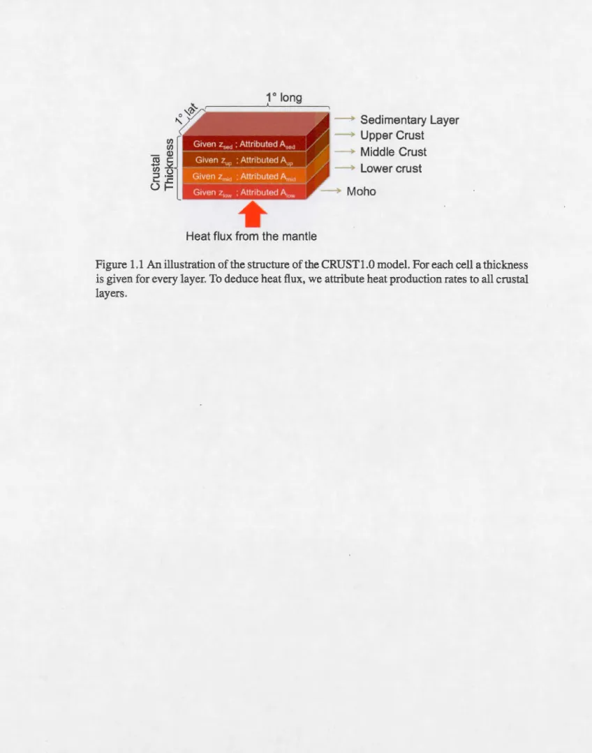
Figure Page 1.1 An illustration of the structure of the CRUSTl .0 model. . . . . . . . . 17 1.2 Globally calculated heat production from borehole data of heat flux

avera-ged over 1 ° x 1 ° cells supposing a constant mantle flow of 15mW m-2 ₁₈

1.3 Four attempts to estimate heat flux on a global scale.

1.4 Eastern Canada calculated heat production from heat flux data averaged over 1 ° x 1 ° cells supposing a constant mantle flux of 15mW m-2

1.5 Four attempts to estimate heat flux on a regional scale.

1.6 Eastern Canada crustal thlckness according to the CRUSTl .0 model in (a)

and according to data (F. Darbyshire, pers. comm) in (b) . 1.7 Active vs steady state cells for our calculations. . . .

1.8 Difference between the models using the heat flow data and the ones using heat productions estimated with CRUSTl.O model in TNUs.

1.9 Comparing local to global calculation methods. . . . . .

19 20 21 22 22 23 24 1.10 We have compared the two models by subtracting the local model from the

global one for both the data deduced maps and the CRUS Tl .0 deduced one. 25

1.11 Effect of rescaling the cell size on the calculation accuracy. . . 2.1 Two variables that illustrate the secular evolution of the Barth.

2.2 World heat flow map combining continental heat flux measurements in the 25 63

continents and plate cooling model for the oceans. . . . . . . . . . . . 64 2.3 Breakdown of the present energy budget of Barth from Jaupart et al. (2014). 65 2.4 Crustal heat production map of the southeastern Canadian Shield calculated

from data. . . . . . . . . . . . . . . . . . . . . . . . . 66 2.5 Difference between observed surface heat flux in the south eastern part of

the Canadian Shield and the values estimated from CRUSTl.0 with the

layered crustal composition model of Huang et al. (2013).

2.6 Crustal heat production map for the Sudbury region. . . . .

ix

67 68

2.7 Relative increase in neutrino flux at the center of a region where crustal heat production is higher than background as a function of the radius of the anomaly relative to crustal thickness. . . . . . . . . . . . 69 2.8 North-South section of the Sudbury Structure inferred from seismic, gra

-vity, and magnetic data. . . . . . . . . . . . 70 2.9 Crustal geoneutrino flux in eastem Canada estimated from CRUSTl.O

crus-tal structure model with concentrations of heat producing elements propo-sed by Huang et al. (2013). . . . . . . . . . . . . . . . . . . . . 71 2.10 Crustal geoneutrino flux in eastern Canada estimated from heat flow data. 72 2.11 Crustal geoneutrino flux map for central Finland estimated from CRUSTl .O. 73 2.12 Crustal geoneutrino flux map for central Finland estimated from heat flow

data. . . . . . . . . . . . . . . . . . . . . . . . . . . . . 74 3 .1 An illustration of the structure of the mode! used to calculate the

tempera-ture profiles. . . . . . . . . . . . . . . . . . . . . . . . . . . . . 81 3.2 Moho temperatures as a function of crustal thickness for different DI and

heat production. . . . . . . . . . . . . . . . . . . . . . . . . . . . 81 3.3 Heat production of the lower crust as a function of crustal thickness for

varying DI and surface heat production. . . . . . . . . . . . 82 3.4 Temperature field contributed by crustal heat producing elements : cross

sections for a 2D crustal belt of infinite length. . . . . . . . . . . . . 82 3.5 An illustration of the crustal structure variation that have been considered. 83 3.6 Temperature contributed by heat production profiles at the centers of belts

as a fonction of their half width. 83

3.7 Vertical temperature profiles at the centers of belts as a function of their half width. . . . . . . . . . . . . . . 84

3.8 Temperature profiles for doubling the thickness. 85

3.9 Temperature profiles as a fonction of crustal thickness with Archean ave -rage heat production. . . . . . . . . . . . . . . 85

3 .10 Temperature profiles as a function of crustal thickness with present day average heat production. . . . . . . . . . . . . . . . . . . 86 3.11 Temperature profiles as a function of depth of the enriched crustal layer. 86 4.1 Radiogenic heat production rate as a fonction of Si02 content in the Sierra

Nevada batholith, from data in Sawka and Chappell (1988). . . . . 138 4.2 Radiogenic heat production rate as a fonction of P-wave velocity in

Pre-cambrian granulite-facies rocks from Finland and Estonia, from data in Joeleht and Kukkonen (1998). . . . . . . . . . . . . . . . . . . 139 4.3 Amplitude of variations of the surface heat flow and the Moho temperature

due to heat production variations in a 10-km thick crustal layer as a fonction of horizontal scale. . . . . . . . . . . . . . . . . . . . 140 4.4 Map of crustal thickness based on the CRUSTl .0 model on a 1

° x

1

°

grid

(Laske et al., 2013). For many cells without seisrnic data, the values for the crustal thickness are based on geological type. . . . . . . . . . . . . 141 4.5 Map of continental heat flux based on;::::; 35,000 unevenly distributed

conti-nental heat flow measurements. . . . . . . . . 142 4.6 Scatter plot of heat flux and crustal thickness. 143 4.7 Plot of surface heat flow as a function of surface heat production for three

different scales in the Canadian Shield and the Appalachians, from Lévy et al. (2010). . . . . . . . . . . . . . . . . . . . . . . . . . . . . . . 144 4.8 Relationship between heat flow and heat production in the United

King-dom, from Webb et al. (1987). . . . . . . . . . . . . . . . . . 145 4.9 Heat flow map of Fennoscandia, from data in Slagstad et al. (2009). 146 4.10 Relationship between heat flow and heat production in Fennoscandinavia,

from Slagstad (2008). . . . . . . . . . . . . . . . 147 4.11 Average crustal heat production as a function of age, from Jaupart and

Ma-reschal (2014). . . . . . . . . . . . . . . . . 148 4.12 Histogram of continental crust thicknesses sampled at 1 ° x 1 °from Laske

4.13 Moho temperature variations in fonction of crustal thickness and differen-tiation index DI for a mean crustal heat production 1.5 µW m-3 represen-ting Archean conditions.

4.14 Total strength of lithosphere as a fonction of crustal thickness. The strength 150

is calculated for Dl= l (undifferentiated) and Dl= 4.5 (differentiated crust).151 4.15. Post-accretion thermal evolution of crust with an initial temperature

ano-maly confined to a lower crustal layer. Results are given for the lower crust (z

=

0.8 x hm). The two temperature components

Tl

and T, (equation 4.15) are also shown. . . . . . . . . . . . . . . . . . . . . . . . . . . 152 4.16 Vertical temperature profiles illustrating the heating of the crust and lithos

-phere by crustal heat sources. . . . . . . . . . . . . . . . . . . . 153 4.17 Variation of temperature at the base of the lithosphere due to crustal heat

production for two different values of the lithosphere thickness, 150 and 220 km. . . . . . . . . . . . . . . . . . . . . 154 4.18 Variation of the lattice component of thermal conductivity as a function of

RÉSUMÉ

Le budget d'énergie de la Terre dépend de la production de chaleur et de son refroi-dissement séculaire. Le flux de chaleur est généralement mesuré dans les trous de forage dans le cadre de prospections minières et pétrolières limitant la couverture de données aux régions économiquement intéressantes. Pour toute autre région, des méthodes alternatives doivent être employées. CRUSTl .0 est un modèle de la croûte terrestre qui a été utilisé pour estimer la production de chaleur de la croûte dans les continents. Nous avons cherché à améliorer les prédictions du modèle en ajustant les productions de chaleur des différentes couches constituants la croûte terrestre. Nos résultats montrent que l'hypothèse d'une pro-duction de chaleur uniforme pour chaque couche crustale n'est pas valide.

Le flux de géoneutrinos peut être directement déduit à partir de la production de chaleur par les éléments radioactifs. Nous avons testé la validité des prédictions faites grâce au modèle CRUSTl .0 en le comparant au calcul basé sur les données de flux de chaleur. Le traitement différentié des couches crustales n'a pas amélioré le flux prédit. Nous avons également tenté une approche de calcul différente ainsi qu'un rééchantillonage dans le but d'augmenter la précision. Pour toutes ces tentatives, l'erreur peut atteindre 81 % par rapport aux valeurs calculées à partir des données de flux de chaleur dans l'Est canadien. Ceci montre que le modèle CRUSTl .0 ne peut pas être utilisé pour prédire le flux de géoneutrinos provenant de la croûte.

La production de chaleur dans la croûte continentale détermine le régime et l'évolution thermique de la lithosphère. Une augmentation de la production de chaleur fait monter les températures lithosphériques alors que la différentiation des éléments radioactifs abaisse les profils de température. Nous avons étudié l'évolution thermique d'une croûte conti-nentale archéenne lors de sa formation. La croissance conticonti-nentale chauffe la lithosphère et fond la croûte terrestre. Lorsque la largeur de ceintures accrétées dépasse les 300 km et que l'épaisseur de la croûte est de 40 km ou plus, la température à la base de la croûte dépasse les 800°C pour une production de chaleur uniforme. Le métamorphisme et la fusion par-tielle produisent une croûte différentiée verticalement ce qui diminue l'effet du chauffage radioactif. Le chauffage de la lithosphère par les éléments radioactifs augmente avec leur profondeur.

Mots clés

Flux de Chaleur

Il

Elements produisant de la chaleur

Il

Budget énergétique

Il

Terre silicatée

I

l

Nombre d'Urey

I

l

Refroidissement du noyau

Il

Refroidissement du manteau

Il

Cratons

Il

Lithosphère

Il

Production de chaleur de la croûte

I

l

Évolution de la croûte

Il

Métamorphisme à haute température

Il

Métamorphisme post-orogenique

Earth's energy budget includes secular cooling and heat production. Surface energy loss is measured by heat flow which can be determined in available boreholes usually drilled for economic purposes. This limits the data coverage to areas of interest for oil and minerai exploration. For regions of insufficient data coverage, heat flow must be estimated by alternative methods. CRUSTl .0 is a global crustal model that has been used to estimate radiogenic heat production in stable continental regions. We have looked at various ways to improve the models by adjusting the heat production of the different crustal layers. Our analysis of this model shows.that the assumption of laterally uniform heat production throughout the continental crust is not valid.

Crustal geoneutrino flux can be directly calculated from radiogenic heat production. We tested the CRUSTl .0 models efficacy at predicting the geoneutrino flow by comparing them to predictions made with heat flow data. A layered crust does not improve the mo-del predictions. We have also tried altemate calculation methods and rescaling. All failed at improving the model's predictions that are off by as much as 81 % in Eastern Canada showing that using CRUSTl .0 fails to predict the geoneutrino flux.

Heat production in the continental crust affects the lithosphere's thermal regime and evolution. Higher heat production increases temperatures, while differentiating the radio-active elements in the upper crust lowers the temperature. We investigated how the width and thickness of the continental crust affected its thermal structure in the Archean. We found that continental growth heats the lithosphere and can melt the crust. For accretio-nary belts, with a total width of over 300 km and a thickness of 40 km, the temperature at the base of a non differentiated crust exceeds 800 °C. The depth of a high heat producing layer augments the temperature increase this layer will generate. As a result the lower crust undergoes metamorphism and partial melts and the radioactive elements are redistributed into the upper crust thus cooling the lithosphere.

Keyword

Heat flow

Il

Heat producing elements

I

l

Energy budget

Il

Bulk silicate Earth

Il

Urey number Il Core cooling I

l

Mantle cooling I

l

Cratons I

l

Lithosphere I

l

Crustal heat production

Il

Crustal evolution Il High temperature metamorphism I

l

Post orogenic metamorphism

The long term thermal evolution of the Barth is constrained by the present energy bud-get. Earth's total heat cornes from two main sources. The first is the secular heat that was stored in the planet during its formation and early evolution. The second source is the heat generated by radioactive decay in the bulk silicate Barth (BSE) comprising both the crust and mantle. The continental crust is enriched in heat producing elements relative to the mantle. The main focus of this study is the distribution of heat producing elements in BSE and the thermal regime of the continental crust.

The amount of radiogenic heat produced in the Barth decreases exponentially with time following the radioactive decay law. Today's total heat loss is about 46±3 TW out of which 19±5 TW is accounted for by heat production and the remainder by secular cooling (Jaupart et al., 2014).

Convection is the most efficient cooling mechanism for an Earth-sized body. Hot and buoyant materials at the bottom of the mantle rise while cold dense materials at the surface sink. This generates large scale displacements in the silicate rocks of the mantle. This al-lows for a mixing of the materials throughout the mantle. The lithosphere can be defined as the upper boundary layer through which the heat transfer mechanism is conduction. The continental lithosphere does not take part in convection while the oceanic lithosphere forms at oceanic ridges and returns to the mantle at subduction zones. Today, continental crust is formed by accumulation of melts from the subducting oceanic lithosphere in back-arc environments. Radioactive elements such as Uranium, Thorium and Potassium are incom-patible with mantle crystalline structures thus accumulating in the continental crust. This concentration of heat producing elements near the surface makes more efficient the evacua-tion of the heat produced. Although the mantle has a much larger mass (~ 67% of Earth's mass for the mantle against ~ 0.4% for the crust) its total heat production is only slightly more than that of the crust.

lithosphere between the spreading centers and the subduction zones. The present rate of heat loss through the sea floor is 32±2 TW as estimated by Jaupart et al. (2015). For the continental crust, only half of the 14 TW heat loss cornes from the mantle. The other half is from heat produced by radioactive decay. Globally, crustal heat production generates from 5.8 to 7.2 TW (Jaupart and Mareschal, 2015). Mantle heat flow is nearly constant under stable continental crust at ~ 15 mW m-2 . The surface heat flow ranges from 15 to 75 m W m-2 in stable continental crust. In tectonically active regions such as rifts (like the East African rift) or continental collision (like the Himalayas) heat flow is much higher due to magma intrusions or thicker crust.

Heat is propagated from the upper mantle to the surface by conduction. According to Fourier's law, the heat flux Q is defined as follows :

Q= -À

ar

az (1)

where À is the thermal conductivity, T is temperature and z is depth. Thermal conductivity is an intrinsic property of the rocks. In stable continental crust, thermal steady state can be assumed. In steady state and without heat production heat flux would be constant through the lithosphere.

The radioactive elements concentrated in the crust produce heat which is then evacuated by conduction near the Earth's surface. The heat flux measured at the surface is the sum of the mantle heat flow and the total crustal heat production which can be expressed as follows:

rz

m

Qo

=

Qm

+

Jo H(z)dz (2)

where Qo and Qm are the heat flux at the surface and at the Moho respectively. H(z) is the heat production rate as a function of depth, and Zm is Moho depth.

There are many reasons to study heat production in the continental crust. First and foremost, heat production is one of the components that determines how temperature varies

with depth in the continental crust. Integrating Fourier's law to obtain the temperature we find:

r

z

l

T(

z)

=

To

+

Jo IQ(

z')

dz'

(3)

where the heat flow with depth Q(z) is determined by equation 2 where we integrate over

z

"

up to a given depth

z

'.

(4) Temperature depends on the vertical distribution of the radioactive elements in the enriched crust. It controls melting, metamorphic processes and mechanical properties.

The study of continental heat flow can also improve our understanding of the global energy budget and gives us some constraints on Earth's thermal reconstruction. During the course of my Masters, we were interested in two problems : How to best estimate crustal heat production in steady state continental crust? What are the implications of crustal heat production for the thermal regime during continental accretion?

First, heat flow can be determined from measurements of temperature profiles in bore-holes or it can be estimated by using a global model derived from seismic data. From the bore hole data, one can get precise estimate of the local surface heat flux. The first method is always preferred but unfortunately it has not been possible to make heat flow measure-ments ail over the Earth's surface, thus the interest of complementing the data by using the second method. We have compared the estimates from seismic models to the heat flow data and tried to adjust the parameters (heat production for the different layers of the seismic model) to reduce the differences with the data where available.

In the second chapter, the outcome from our models are compared with results from different other studies in a more general context including the present day comprehension of mechanisms of heat loss and partition of heat sources between the continental crust and mantle. Earths secular and radiogenic heat production are discussed as a part of Earth's heat

budget. The CRUST models serve to estimate the continental crustal heat and neutrino production. The mantle heat and neutrino contributions to the surface flux are discussed afterwards.

Then, we looked at the thermal regimes of the crust during craton formation. Long belts

of crustal material accrete together to form continents. We calculate the temperature profile for accretion belts of various widths and thicknesses. These profiles inforrn us about partial melts and other temperature controlled phenomena.

In the Jast chapter, the calculations made above are compared with large data sets on heat flow and heat production. Herein, we discus crustal stratification estimates and heat production in a number of geological provinces.

Ca

lc

ulating crustal heat production and

geo-neu

t

rino flux in stable continents.

1.1 Global Crustal Model

In this section, we illustrate the tests that we made with the CRUSTl .0 model to esti -mate surface heat flow and geoneutrino flux. CRUSTl.O is a global crustal model based on seismic data and crustal type and age. Excluding ice and water, the crust is divided in six layers, three for the sediments and three for crystalline crust. The Earth is divided in cells

of 1

° latitude per 1

°

longitude and the model gives a thickness and physical properties for each crustal layer in every cell.

We shall calculate for each cell the crustal heat production and surface heat flux and compare the result with heat flux measurements. The motivation for this approach is that if the model matches well with the available data, it can be used with a certain confidence to estimate heat flow in thermally equilibrated areas where data are unavailable. The objective is to find the heat production rates that will provide a good fit.

1.2 Comparing Heat Flow

ln steady state the surface heat flux is the surn of the mantle heat flux and the total crustal heat production. We attribute a heat production rate to each crustal layer and inte-grate over crustal thickness to obtain the component of the surface heat flow contributed by crustal heat production. We attributed heat production rate to all sedimentary layers adding an average mantle heat flow Qm gives us the surface heat flux that can be compared with measured heat flux as shown in equation 2 (page 2).

6 Qo

=

Qm

+

[ A;&;

1

Where A; and &; are the heat production rate and thickness of the crustal layer i.

(1.1)

The heat flow data are unevenly distributed. To compare with the mode!, we averaged the data points over 1 °xl O

cells thus also reducing the weight of anomalous individual measurements. We can then compare all cells with data to cells from the model in stable continental areas where transient thermal perturbations are negligible.

We tried different heat production rates for the different crustal layers. As a first ap-proximation, we tried a global crustal average for the heat production of 0.89 µW m-3 , as calculated by Rudnick and Gao (2014). We then made different attempts with a differen-tiated crust. In the. first attempt, we used the heat production rates for crustal layers from Rudnick and Gao (2014) and 0.9 µW m-3 _{for sediments. The results follow more closely} the crustal thickness maps than the heat production maps.

We also varied the heat production rates to find the set of A; that minimizes the root

mean square (RMS) difference with the datl. This gave the optimized model. We calculated the optimal set of parameters separately for each region of analysis. This yielded the maps 1.3c for the global optimization and 1.5c for Eastern Canada's optimization. The optimal values obtained for both global and regional scales are listed in table 1.1 where we assumed

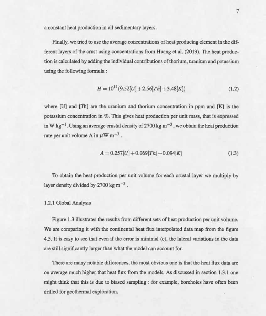
a constant heat production in all sedimentary layers.

Finally, we tried to use the average concentrations of heat producing element in the dif-ferent layers of the crust using concentrations from Huang et al. (2013). The heat produc-tion is calculated by adding the individual contributions of thorium, uranium and potassium using the following formula :

H

=

1011(9.52[U] + 2.56[Th] +3.48[K]) (1.2)

where [U] and [Th] are the uranium and thorium concentration in ppm and [KJ is the potassium concentration in %. This gives heat production per unit mass, that is expressed in W kg-1. Using an average crustal density of 2700 kg m-3, we obtain the heat production

rate per unit volume A in µW m-3 .

A

=

0.257[U] + 0.069[Th] + 0.094[K] (1.3)

To obtain the heat production per unit volume for each crustal layer we multiply by layer density divided by 2700 kg m-3 .

1.2.1 Global Analysis

Figure 1.3 illustrates the results from different sets of heat production per unit volume.

We are comparing it with the continental heat flux interpolated data map from the figure

4.5. It is easy to see that even if the error is minimal (c), the lateral variations in the data are still significantly larger than what the model can account for.

There are many notable differences, the most obvious one is that the heat flux data are on average much higher that heat flux from the models. As discussed in section 1.3.1 one rnight think that this is due to biased sampling : for example, boreholes have often been drilled for geothermal exploration.

But averaging the points over cells of the same dimensions as the model reduces signi-ficantly the weight of those data points as can be observed in figure 1.2. Then there are the contrasts that are much greater in the data than in any of the model. The high heat flow regions that have a higher surface flux than the models are not in equilibrium and will not be discussed further. The low heat flux areas, specifically the shields have a lower flow than any of the models because their heat production is very low even though the crust is thick. In other words, continental shields and low heat flow regions are not visible because the model assumes incorrectly a constant heat production in each layer. On a large scale, all the models exhibit the same patterns as the crustal thickness map shown in Figure 4.4 rather than those of heat fl.ow data.

1.2.2 Regional Analysis

We then tested the model on a regional scale over Eastern Canada where there are many heat fl.ow data. the region has two distinct crust types : the Shield and the Appalachians. Looking at the interpolated data map of figure 2.4 one can see that the northern older regions are characterized by very low heat production. The highest heat production is in the southeasternmost corner of Canada : the Appalachians. Several small scale areas of high heat production can also be observed. As in the global analysis, for the purpose of comparison, all data points have been averaged on cells identical to those of the model and shown in figure 1.4.

The difference between the Shield and the Appalachians is not seen in any of the tests and the calculated heat flux is directly proportional to crustal thickness. Because the crus-tal thickness of the Appalachians is close to that of the shield, see figure 1.6 one can not distinguish one from the other if the heat production is uniform throughout the entire crust. The Rudnick and Gao (2014) heat production rates generates a model that suggests a hi-gher heat production on average in the Appalachians than in the Shield, but the contrasts in heat production are much larger for the data maps especially in central Quebec. We have minimized the root mean square difference to obtain the optimal model. Sorne of the low

heat production zones are better represented but the high heat production remains signi

-ficantly higher in the data. On the other hand, the model resulting from concentration of heat producing element of Huang et al. (2013) attributes well for the high heat producing

areas notably the Appalachian orogen but fails in the older Shield areas with very low heat production.

In the data, variations of over 35m W m-2 in the surface heat flux can occur over less than 100 km(,=::; 1 cell) which is never seen in the models that are very smooth in compa-rison. The variations in all models are spread out over large distances and show no abrupt changes comparable to those in the data.

We have also compared the model crustal thickness to that from seismic data. Looking

at the two maps of crustal thickness in Eastern Canada one can see that the crustal thick

-ness is accurate in that region. Therefore the discrepancy in heat productions is not due to an error in predicted crustal thickness but only due to the calculation method. We have concluded that assuming a constant heat production within each layer of the crust is not

valid. Thus the heat production is higher in the Appalachian not because the highest heat producing layer is thicker than in the Shield but because the concentration of heat produ-cing elements is higher within the same layers. A similar conclusion applies to the Shield for low heat production. It is also more natural for small scale high heat flow anomalies to

coincide with a large increase in concentrations rather than abrupt thickening of a layer. If crustal thickness is not the issue when modeling heat production, then the only re-maining parameter is the heat production rate. Bach value used represents an average for

a given crustal layer. Even if the average is accurate, the heat production rates will still vary laterally within the layer over large and small scales. The only way to get additional

information on these variations is by heat flow measurements. This is not due to a short

-coming of CRUSTl.O which contains no information on heat production, but to the wrong

1.2.3 Conclusion

Both the global and regional analysis show large discrepancies emerging in areas of low heat production characteristic of continental shields. In the multilayered models, the Appalachians can barely be distinguished from the shield and the amplitude of the dif-ference in heat productions is significantly less in the model than in the heat production deterrnined from the heat flow measurements. This shows the obvious lack of lateral va-riability of scale and amplitude in the CRUSTl .0 models that can not account for lateral changes in concentrations of heat producing elements. The mode! assumes that the heat production rate remains constant within each crustal layer which cannot show the lateral variations in heat flow that have been observed.

1.3 Bstimating Crustal Geoneutrino Flux

As described in Fiorentini et al. (2005) disintegration of each radiogenic element pro-duces heat and neutrinos in known amounts. We can thus deduce geoneutrino flux from heat flow provided that we know the ratios of the concentrations in Heat producing ele-ments. Assuming a perfectly spherical geometry of Barth and integrating over it's volume, the total geoneutrino flux at any point is obtained by :

<I>i(r

)

= -

1 (

AJf'

)

p(?) dV'

,

47r

Jv

I

r' -

r

l2

(1.4)

where Ai is the luminosity (number of anti-neutrinos per unit time produced inside Barth) per unit mass for isotopes 238U and 232T h, p is the local density. r' and rare the location of the source and the observation point, respectively. Here we only consider isotopes 238_{U and} 232_{Th because both} 4_{°K and} 235_{U produce neutrinos below the 1.8 MeV threshold of} de-tection in liquid scintillatior (Fiorentini et al., 2005). But, given the elemental abundances ratios that are better known, one can deduce the amount of 4°K and 235U once the absolute abundance of 238U and 232Th are measured.

Because we are only interested in calculating the crustal component of the neutrino flux <I> in terms of heat production H from the crust, we integrate only over the volume of Earth's crust.

<I>( 8' </>)

=

~4a2 {zm dz' {2n d</>' {n d case' H(z' ':'' </>')'

rr Jo

Jo

Jo

RPP'

(1.5)

where the factor y is the conversion factor of crustal radioactivity to neutrino production rate, a is the radius of the Barth, 8 and </> are, respectively, the colatitude and longitude at the observation point, z the depth, Zm the Moha depth, Rpp' is the distance between the source (p') and the observation point (p) and H is the crustal heat production. Here the unchanging factor y assumes a constant mass ratio of the heat producing elements. For Th/U = 4 and K/U =12,000, we obtain

y=

0.65 x 1012 J-1. Neutrino Flux is expressed in terrestrial neutrino units (TNU). Where one TNU corresponds to one event recorded per year of exposure in a detector of 1032 protons.

To calculate the global neutrino flux, we calculated the flux from equation 1.5 for each of CRUSTI .0 model cells. We separated the near and the far field regions. For two cells that are far apart, we mak:e a point source approximation. Rpp' is the distance between the centers of both cells. For neighboring cells, the point approximation is not valid, but we can neglect Earths curvature when we integrate over all Rpp'· We compared two different calculation methods for this in subsection 1.3.2.

Because of the geoneutrino radial flux and Earth's geometry one needs to have a heat flow value for each cell off the model to get an accurate estimate of the crustal geoneutrino flux. Because many cells do not contain heat flow data, we extrapolated the data where possible. In areas where the crust is not in thermal equilibrium and heat production cannot be estimated from heat flow, we used heat flow estimates from the CRUSTl .0 model. For cells in continental stable crust where heat production is calculated with confidence we can approximate the difference in geoneutrino flux from heat production estimated with the

CRUSTl .0 model and from the calculated heat flux.

We subdivided the world map in three crustal categories, oceanic, active and stable continental crusts. We consider as oceanic, ail the cells that have an oceanic crustal age. The distinction between stable and active crustal areas are based on heat flow and crustal thickness. We consider as active the continental crust thinner than 25 km or thicker than 60 km and/or regions with heat flux higher than 65 mW m-2 . This classification is illustrated in figure 1.7 where the areas in green are the only ones where heat flow data can be used for estimating neutrino flux.

From this comparison, we get an estimate of the magnitude of the error made by the model using CRUSTl.O alone·to predict neutrino flux.

1.3.1 Varying Heat Production

The neutrino flux maps are much smoother than the heat production ones. The intensity of the neutrino flux is inversely proportional to the square of the distance as shown in equation 1.5, while the heat flux is proportional to

z/

R3.

For the far field, we are using a point source approximation so we can only use one heat production per cell of the model. We have looked at the effect of changing the ave-rage crustal heat production on the scale of the difference it will produce with the model using heat flow data where available. We subtracted the neutrino flux calculated using only CRUSTl.O estimated heat flux from the one using data where available in stable crust for each of the difference maps in figure 1.8. The differences are in TNU units. We use TNUs in this section to compare with the neutrino detection resolution in TNUs.

In the previous section we have seen that the model does not account well for the regions with low concentrations of heat producing elements in the crust that often are found in Shields. Therefore we expect to overestimate the neutrino production in those areas. In figure 1.8a the global average heat production is estimated at 0.67 µW m-3 _the

CRUSTl .0 deduced model seems to underestimate the data deduced one unlike what we would expect. The following figure 1.8b assumes a 0.75 µW m-3 of global heat production average and what shows well here is that all the areas where the neutrino difference is very positive, are near the stable to active crust boundary. In other words the areas where the crust is stable but the neutrino flux modeled with data are higher that the ones coming from CRUSTl .O. This shows that the heat production rate of those areas is underestimated. The only areas where the heat flow is higher than in the model are in active crustal zones. This is coherent with the continental heat production estimates of 0.79 to 0.95µW m-3 _by Jaupart and Mareschal (2014). Both figure 1.8c with an average heat production of 0.83 µW m-3 and figure 1.8d with 0.90 µW m-3 are within that range and show significantly smaller areas with positive error and a more of the expected negative error.

In the last figure 1.8e, we have calculated the crustal average heat production for each cell assurning concentrations for each layer from Huang et al. (2013). The resulting dif-ference map is very sirnilar to the results from figure 1.8d with 0.90 µW m-3 _{, showing} small differences in the Canadian and Baltic Shields but larger ones in Asia.

1.3.2 Varying Calculation Method Used for the Model

We have calculated the neutrino flux using two different methods. The first one that we call global, uses a cylindrical approximation to integrate over the volume of a crustal column in the near field. The second method that we call local, performs a two dimensional integration over the surface of the cell and multiplies by crustal thickness in the near field.

The results based on data (figures 1.9a and 1.9b) display greater variation than the ones based on crustal thickness (figures 1.9c and 1.9d). The differences between the data and crustal thickness based models (figures 1.9e and 1.9f) are as high as 25 TNUs for both calculation methods. This is an error larger than the absolute value of the flux in the northern Quebec region. In the surroundings of the Sudbury Neutrino Observatory (SNO) the error is low. The very old northern Quebec craton core is where the error is largest.

Figure 1.10 shows the north to south gradient to be due to the cylindrical approximation and the size variation of cells with latitude. Comparing the two calculation methods in figure 1.10, we note that th~ difference is less than 1 TNU over most of the region. This implies that the error of the cylindrical approximation is small. The calculation method does not affect the results of the model when predicting the neutrino flux.

1.3.3 Varying the Sampling Square Size

We also looked at the effect of rescaling the size over which we integrate to have a better

accuracy in the neutrino flux. Instead of using the 1 ° latitude per 1 ° longitude division we

tried dividing the Earth in 0.5''' per 0.5° and 0.25° per 0.25° sized cells.

The increased "accuracy" has no effect on the model. Increase in precision of calcula-tion does not show on the smoothed (figures 1.11) highlighting once a gain the systematic

error in the models use.

1.3.4 Power Spectra

We have compared the power spectra of the heat flow and crustal thickness for the North American continent. Both data sets were placed on a 1 ° x 1 °to calculate the power

spectra over the same range of wavenumbers. Unfortunately both data sets do not have

sufficient spatial resolution to make a comparison over a large range of wavenumbers. The comparison shows that crustal thickness is smoother than the heat flow field. The spectral slope (dlog(P) / dlog(k)) of the crustal thickness power spectrum (2.3) is larger than that of the heat flow (1.5) resulting in a smoother field. Partly, this is because small scale features

on the Moho cannot be resolved by seismic data. But, this is also an artifact due to the elimination in the crustal model of differences in thickness between cells that have the

same geological type. The heat flow integrates heat production vertically and horizontally over a cone whose radius increases with depth, also resulting in smoothing of the field but not in annihilation of the sborter wavelength. Over North America, heat flow and crustal

thickness are not correlated (r=0.15). Worldwide, the correlation between heat flow and crustal thickness is even slightly negative (r==-0.1) (Mareschal and Jaupart, 2013).

1.3.5 Conclusion

Regardless of heat production values used, the models using CRUSTl .0 predictions are off by more than 25 TNUs in continental Shields. The error remains as great with improved calculation methods and accuracy. CRUSTl .0 can not be used to accuratly predict neutrino flux. This is developed in the following chapter as a part of larger discussion on heat flow.

Average Heat Productions per Unit Volume (µW m-3₎

Madel sedimentary

I

upper crust

I

middle crust

I

lower crust (a) Single-layered

(b) 1 st Multilayered (c) Optimized Global Estem Canada (d) Concentrations:j: t Rudruck and Gao (2014) :j: Huang et al. (2013) 0.9 1.5 1.5 0.98 0.89 t l.6t 0.96t 0.18t 1.4 0.8 0.6 1.4 0.2 0.1 1.67 0.78 0.19

- Upper Crust

- Middle Crust

- Lower crust

•

Heat flux from the mantle

Figure 1.1 An illustration of the structure of the CRUSTl .0 model. For each cella thickness

is given for every layer. To deduce heat flux, we attribute heat production rates to all crustal

12o·w eo·

w

o

·

0 10 15 20 25 30

eo

·E 12o·E

35 40 45 50 mwm-2 150

Figure 1.2 Globally calculated heat production from borehole data of heat flux averaged

12o·w so·w o· so·e 12o·e 30"N · o· -3o·s (a) 12o·w SO'W o· SO'E 12o·e (b) (c) 12o·w SO'W o· so·e 120'E 30'N -o· -30'5 -mwm-2 0 10 15 20 25 40 45 50 150 (d)

Figure 1.3 Four attempts to estimate heat flux on a global scale where (a) is obtained using a crustal average heat production of 0.89 estimated by Rudnick and Gao (2014) (b), (c)

and (d) are using a differentiated crustal heat production with the heat production rate of each crustal layer is that estimated by Rudnick and Gao (2014) in (b) optimized to reduce the average difference with the data in (c) and is deduced from estimated concentrations of heat producing elements by Huang et al. (2013) in (d) the heat production rate values for each model are shown in table 1.1

11o·w 1oo·w go·w ao·w 7o·w

mwm-2

0 10 15 20 25 30 35 40 45 50 150

Figure 1.4 Eastern Canada calculated heat production from heat flux data averaged over 1 °

0 10 15 20 25 30 35 40 45 50 150 0 10 15 20 25 30 35 40 45 50 150

(a) (b)

0 10 15 20 25 30 35 40 45 50 150 0 10 15 20 25 30 35 40 45 50 150

(c) (d)

Figure 1.5 Four attempts to estimate heat flux on a regional scale where (a) is obtained using

a crustal average heat production of 0.89 mW m-2 estimated by Rudnick and Gao (2014) (b), (c) and (d) are using a differentiated crustal heat production with the heat production

rate estimated by Rudnick and Gao (2014) in (b) optimized to reduce the difference with the data in (c) from estimated concentrations of heat producing elements by Huang et al.

(2013) in (d). The heat production values for each attempt are shown in table 1.1.The

55"N

SO"N

45.N

10 15 20 25 30 35 40 45 50 55 60 10 15 20 25 30 35 40 45 50 55 60

(a) (b)

Figure 1.6 Eastern Canada crustal thickness according to the CRUSTl .0 model in (a) and according to data (F. Darbyshire, pers. comrn) in (b)

210· 250· 310·

o

·

50· 100· 150·

Figure 1.7 Active vs steady state cells for our calculations. The cells are BLUE for oceanic crust, GREEN for stable continental crust, and RED for active continental crust. Stable continental crust is defined as having a heat flow below 65 mW m-2 and crustal thickness between 25 and 60 km.

20· o· -20· (a) (b) 210· 2so· 310· o· so· 100· 210· 20"N o· 2o·s (c) (d)

15o·w10o·w 5o·w o· 50"E 1oo·E 15o"E

so· 100· 1so·

-25 -20 -15 -10 -5 0 5 10 15 20 25 (e)

Figure 1.8 Difference between the models using the heat flow data and the ones using heat productions estimated with CRUST1 .0 model in TNUs. In each case we used a dif-ferent heat production for the crust. (a) average hp

=

0.67 µW m-3 (b)average hp

=

0.75

µW m-3 (c) average hp

=

0.83 µW m-3 (d) average hp

=

0.90 µW m-3 (e) using Huang

24 29 34 39 (a) 24 29 34 39 (c) -25 -20 -15 -10 -5 (e) 44 49 44 49 54 54 10 TNU 59 TNU 59 TNU 15 24 29 34 39 (b) 44 49 54 TNU 59

-

~

-

J

59 TNU 24 29 34 39 44 (d) ]~ :--- - - . -25 -20 -15 -10 -5 (t) 49 54 TNU

~

-

_;...

--""

10 15

Figure 1.9 Comparing local to global calculation methods. AU the figure on the right hand

side are produced with the global model. The ones one the left are from the local model. In the first row, we presented the models using heat flow data where available, in the second

one, the model using only CRUSTl .0 values and in the last row, we have subtracted the

TNU

-

-

-

--11111

-1.0 -0.5 0.0 0.5 1.0 1.5 (a) -1.0 -0.5 0.0 (b) 0.5 1.0 TNU 1.5

Figure 1.10 We have compared the two models by subtracting the local mode! from the global one for both the data deduced maps in (a) and the CRUSTl.0 deduced one in (b).

(a) (b) (c)

Figure 1.11 Effect of rescaling the cell size on the calculation accuracy. (a) the crustal model with a cell of 1 °square; (b) resized to 0.5 °andin (c) resized to 0.25 °.

The Earth's Heat Budget, Crustal

Radioac-tivity and Mantle Geoneutrinos

Jean-Claude Mareschal

GEOTOP, University of Quebec at Montreal, POB 8888, sta. downtown, Montreal,

H3C3P8, Canada - mareschal.jean-claude@uqam.ca

Claude Jaupart

Institut de Physique du Globe de Paris, 1, rue Jussieu -75238 Paris cedex 05, France

- jaupart@ipgp.fr Lidia Iarotsky

GEOTOP, University of Quebec at Montreal, POB 8888, sta. downtown, Montreal, H3C3P8, Canada - iarotsky.lidia@courrier.uqam.ca

Mareschal, J.C., Jaupart C., Iarotsky L., 2016. The Earth's Heat Budget, Crustal Radioactivity and Mantle Geoneutrinos, In : Ludhova, L. (Ed.), Geoneutrinos. ISBN 978-83-944520-1-8

Abstract

Studies of the Barth's thermal evolution have progressed slowly because of the fonda-mental difficulty of dealing with a highly heterogeneous system that continuously changes its upper boundary conditions and internai distribution of heat sources. Here, we review current understanding on the mechanisms of heat loss and on the partition of heat sources between the continents and the convecting mantle. We evaluate the various items, including the core heat loss, in the energy budget of our planet with emphasis on the methods used to deterrnine them and their uncertainties. The total energy Joss of the Barth 46

±

3TW is well established by heat flow measurements in the continents and well-tested physical models for cooling of the sea floor. This energy loss is balanced by heat production of radioactive elements in the crust and in the mantle and by secular cooling of the mantle and core. The amount of heat due to radioactive decay in the continental crust can be de-termined quite accurately (i.e., within

±

10%) and accounts for a fraction of the Barth's total heat generation that may be as large as 50%. In contrast, heat generation in the Bar-th's mantle is poorly constrained, which limits our understanding of the BarBar-th's convective engine. For geologists, the main challenge is not to determine the Barth's secular cooling rate because it can be determined directly from ancient lava samples, but to understand the physical controls on plate tectonics and continental growth, which act to deplete the Bar-th's mantle in heat producing elements. On land, heat flux measurements record the total crustal heat production without knowledge of ail the rock types present including those of lower crustal horizons that are beyond the geologist's reach. Geoneutrino observations and measurements of the Barth's surface heat flux are both needed to narrow down the uncertainties on the breakdown of the energy budget. They complement each other in the interpretation of the geoneutrino signal at observatories located on land where the crustal contribution is much larger than the mantle one and must be determined independently.

Keyword

number

I

l

Core cooling

Il

Mantle cooling

2.1 Introduction

Secular cooling has always been a central issue in the Barth Sciences because our pla-net's present state and geological activity result from more than four billion years of evolu-tion. In the 19th century, advances in the theory of heat conduction and in thermodynamics were immediately applied to questions regarding the interna! structure and thermal evolu-tion of the Barth. When Fourier first published his Théorie Analytique de la Chaleur, he realized that the temperature inside the Barth had to be very high and he thought that the Barth had retained most of the heat from its formation (Fourier, 1820, 1824). Lord Kelvin reached the same conclusion with his famous calculation of the age of our planet (Thom-son, 1864). His result was not consistent with geological evidence. The strong controversy that ensued is exemplary of the di vide still to be bridged between physicists and geologists. At the tirne of Fourier and Kelvin, the Earth's temperature gradient was estimated to be in the range 20-30 K km-1_{, which is surprisingly accurate. From this value, Kelvin deduced} that our planet was not much older than 100 My. His calculation rested on the assumptions that the Barth is cooling by conduction and that there are no sources of heat inside it, which are not valid. He rnight not have followed this approach if he had paid more attention to the variability of surface heat flux. Even in his days, temperature measurements in deep mine shafts and galleries showed that the heat flux varies by large amounts at Earth's surface, which is not consistent with a uniform cooling model for the planet. From our present-day perspective, the most serious flaws of Kelvin's model are that it relied on a value for the temperature gradient in continents and that it did not account for the fondamental

diffe-rences that exist between oceans and continents. We know now that heat generated locally

by the decay of uranium and thorium in the crust is by far the largest contribution to the continental heat flux. The Barth is losing most of its heat through the sea floor and it is in the oceans that the hypothesis of a static planet cooling by conduction was invalidated in the most spectacular manner. As we shall see, the fondamental dichotomy of the

mecha-nisms of heat loss in continents and oceans has hampered progress in part because it took a long time to secure reliable measurements at sea and in part because heat flux measure-ments on land had to be complernented by determinations of radiogenic heat production in crustal rocks.

The discovery of radioactivity by Becquerel in 1896 completely changed our unders-tanding of the Barth's energy budget. The importance of long-lived radioactive elements was rapidly appreciated (Strutt, 1906; Joly, 1909; Holmes, 1915a,b). Attention was soon focussed on the distribution of heat producing elements within the Barth and only much later turned to the issue of heat transport by convection. With almost no evidence for the early Barth's thermal state, some authors even entertained the notion that the Barth had been heating because of radioactivity (Halines, 1931). Although it is now clear that this is not so, the contribution of secular cooling to the energy budget remains very poorly constrained. Another consequence of the discovery of radioactivity is that the heat released in rocks by the decay of uranium, thorium and potassium can be compared with the heat flux and used to constrain the composition of the Earth. Three years before the discovery by seismology of the Mohorovicic discontinuity separating the crust and the mantle, Strutt (1.906) used this method to conclude that the Barth's crust could not be thicker than 60km. These studies set the course of research on surface heat flow and on. the cooling of the Earth very early on. Heat flow studies provide the strongest constraints on the total heat loss of the Barth but, except for heat production in the continental crust, they can not resolve the other components of the energy budget (mantle and core cooling, mantle heat production). It is hoped that geoneutrino observations will provide a direct measurement of the concentration of uranium and thorium in the Barth's mantle, Jead to better constraints on mantle heat production, and reduce the uncertainty on the secular cooling of the core and mantle. Geoneutrino and heat flow studies complement one another in another impor-tant area. In continental observatories, the neutrino flux is dominated by the local crustal radioactivity. Accounting for this contribution is a major challenge because of the extre-mely heterogeneous structure of the Barth's crust at all scales and the difficulty in relating

a geophysical model of crustal structure to the amount of radioactive elements. The surface heat flux directly records the total crustal heat production beneath the measurement site, from which one can infer uranium and thorium contents with little error.

In this chapter, we begin by reviewing the present understanding of Earth's secular evolution and the debates on the mantle processes that have shaped the Barth. We then briefly summarize how the total heat Joss of the Barth has been calculated. Outstanding questions on how the tectonic regime of our planet has evolved are best tackled from a thermal perspective and rel y on an analysis of the secular evolution of mantle convection, which requires a breakdown of the energy budget of the Earth's mantle. We show that uncertainties on the main items of this budget are crippling and discuss how geoneutrino studies could help. Turning to crustal heat production, we demonstrate how the total crustal neutrino flux can be determined directly from heat flux measurements in stable continents. In a final section, we discuss different ways to calculate the crustal geoneutrino signal with applications to the Sudbury neutrino observatory, Canada, and the proposed site at Lena in Finland.

2.2 The Secular Cooling and Evolution of Barth

2.2.1 Initial Conditions

Initial conditions are required for thermal calculations but, more importantly, provide the most natural perspective to evaluate how the Earth's current dynamic regime has super-seded previous ones. There is no doubt today that our planet started from very high initial temperatures. The earliest phases of its existence were marked by several independent pro-cesses which all released large amounts of energy. The end of accretion probably saw a giant impact which led to the formation of the Moon and heated the planet by as much as 7000 K, such that parts of the Barth were vaporized (Cameron, 2001; Canup, 2004) . This makes irrelevant the question of whether the Barth was melted from impacts during the accretion sequence. Following accretion, large quantities of iron sank through the Earth's