THÈSE
THÈSE
En vue de l'obtention du
DOCTORAT DE L’UNIVERSITÉ DE TOULOUSE
DOCTORAT DE L’UNIVERSITÉ DE TOULOUSE
Délivré par Institut National Polytechnique de Toulouse Discipline ou spécialité : Informatique
JURY
Stefanie Hahmann, Professeur à l'Institut de Technologie de Grenolble Eckehard Steinbach, Professeur à la Technische Universität München
Mathias Paulin, Professeur à l'Université de Toulouse
Wei Tsang Ooi, Asistant Professeur à la National University of Singapore Géraldine Morin, Maître de Conférences à l'Université de Toulouse Romulus Grigoras, Maître de Conférences à l'Université de Toulouse
Ecole doctorale : Mathématiques, Informatique et Telecommunications de Toulouse Unité de recherche : Institut de Recherche en Informatique de Toulouse
Directeur(s) de Thèse : Mathias Paulin
Rapporteurs : Stefanie Hahmann, Eckehard Steinbach
Présentée et soutenue par Sebastien Mondet Le 8 juin 2009
A
DAPTIVE
M
ODELING AND
D
ISTRIBUTION
OF
L
ARGE
N
ATURAL
S
CENES
Sebastien Mondet
Thesis Committee:
Supervisor: Mathias Paulin (University of Toulouse)
Co-advisors: Géraldine Morin (University of Toulouse)
Romulus Grigoras (University of Toulouse)
Wei Tsang Ooi (National University of Singapore)
Examiners: Stefanie Hahmann (Grenoble Institute of Technology)
Author: Sebastien Mondet
Advisors: Mathias Paulin, Géraldine Morin, Romulus Grigoras
Abstract:
This thesis deals with the modeling and the interactive streaming of large natural 3D scenes. We aim at providing techniques to allow the remote walkthrough of users in a natural 3D scene ensuring botanical coherency and interactivity.
First, we provide a compact and progressive representation for botanically realistic plant models. The topological structure and the geometry of the plants are represented by generalized cylinders. We provide a multireso-lution compression scheme, based on standardization and instantiation, on difference-based decorrelation, and on entropy coding.
Then, we study efficient transmission of these 3D objects. The proposed packetization scheme works for any multiresolution 3D representation. We validate our packetization scheme with extensive experiments over a WAN (Wide Area Network), with and without congestion control (Datagram Congestion Control Protocol).
Finally, we address issues on streaming at the scene-level. We optimize the viewpoint culling requests on server-side by providing an adapted data-structure and we prepare the ground for our further work on scalability and deployment of distributed 3D streaming systems.
Keywords: Streaming, Plant models, Multiresolution, Progressive coding, Progressive transmission, Networked Virtual Environment
Auteur : Sebastien Mondet
Encadrants : Mathias Paulin, Géraldine Morin, Romulus Grigoras
Résumé :
Cette thèse traite de la modélisation et la diffusion de grandes scènes 3D naturelles. Nous visons à fournir des techniques pour permettre à des util-isateurs de naviguer à distance dans une scène 3D naturelle, tout en assur-ant la cohérence botanique et l’interactivité.
Tout d’abord, nous fournissons une technique de compression multi-résolution, fondée sur la normalisation, l’instanciation, la décorrélation, et sur le codage entropique des informations géometriques pour des modèles de plantes.
Ensuite, nous étudions la transmission efficace de ces objets 3D. L’algorithme de paquétisation proposé fonctionne pour la plupart des représentations multi-résolution d’objet 3D. Nous validons les techniques de paquétisation par des expériences sur un WAN (Wide Area Network), avec et sans contrôle de congestion (Datagram Congestion Control Proto-col).
Enfin, nous abordons les questions du streaming au niveau de la scène. Nous optimisons le traitement des requêtes du côté serveur en fournissant une structure de données adaptée et nous préparons le terrain pour nos travaux futurs sur l’évolutivité et le déploiement de systèmes distribués de streaming 3D.
Mots-clés : Streaming, Modèles de plantes, Multirésolution, Codage pro-gressif, Transmission progressive, Environnement Virtuel Distribué
Autor: Sebastien Mondet
Supervisores: Mathias Paulin, Géraldine Morin, Romulus Grigoras
Resumen:
Esta tesis se refiere a la modelización y la distribución de escenas 3D in-teractivas naturales. Nuestro objetivo es proporcionar la tecnología para permitir a los usuarios navegar en una escena 3D natural a distancia al tiempo que se garantiza la coherencia botánica y la interactividad.
En primer lugar, se proporciona una técnica de compresión multiresolu-ción, sobre la base de la normalizamultiresolu-ción, la instanciamultiresolu-ción, la decorrelamultiresolu-ción, y la codificación entropica de la información geométrica de modelos de plantas.
A continuación, se estudia la transmisión eficaz de estos objetos 3D. El algoritmo de paquetización que proponemos funciona con la mayoría de las representaciones multiresolución de objetos 3D. Validamos las técnicas paquetización por experimentos en una Red de Área Amplia (WAN), con y sin control de la congestión (Datagram Congestion Control Protocol). Por último, se aborda las cuestiones del streaming al nivel de la escena. Optimizamos el procesamiento de consultas en el lado del servidor, pro-porcionando una estructura de datos adaptada y preparamos el terreno para nuestro trabajo futuro sobre la escalabilidad y el despliegue de los sistemas distribuidos de streaming 3D.
Palabras clave: Streaming, Modelos de plantas, multiresolución, codifi-cación entropíca, transmisión progresiva, Entorno Virtual Distribuido
TEXT:
大规模自然场景的自适应建模和分发
本论文研究大规模三维自然场景的建模和交互性流传输,
目标是使用户能够在三维自然场景中远程漫游,并且保
证交互性和植物的真实性(植物学意义上与真实植物保
持一致)。
首先,本文为(植物学意义上严格)真实的植物模型提
供一个紧凑和渐进
(progressive)的表现方式。
此模型中,植物的拓扑结构和几何特性以通用柱体来
表示。本文提供了一个基于标准化和实例化, 差值解
相关, 和熵编码的多分辨率的压缩体系。
然后,本文研究了上述三维物体的高效传输。文中给出
的打包体系适用于任何多分辨率的三维表现方式。本文
用广域网上大量的实验(实验中既用了有拥塞控制的协
议,也用了无拥塞控制的协议)来验证了这个打包机制。
最后,本文解决了场景层面上的流传输中的一些问题。
文中提供了一个改进的数据结构来优化服务器端的视
点挑选
(culling)操作这为我们将来研究分布式三维流媒
体传输系统的可扩展性和部署问题打下了基础。
Autor: Sebastien Mondet
Indrumatori: Mathias Paulin, Géraldine Morin, Romulus Grigoras
Rezumat:
Teza trateaz˘a modelizarea s,i difuzarea scenelor 3D naturale de mari
dimen-siuni. Aceate lucrare propune tehnici ce permit utilizatorilor s˘a navigheze
de la distant,a într-o scen˘a 3D natural˘a, asigurând în acelas,i timp coerent,a
botanica s,i o bun˘a interactivitate.
Într-o prim˘a etap˘a, prezentam o tehnic˘a de compresie multirezolut,ie,
bazat˘a pe normalizarea, instant,ierea, decorelarea s,i codajul entropic al
informat,iilor geometrice privind modelele de plante.
În continuare, studiem transmisia eficace a acestor obiecte
tridimen-sionale. Algoritmul de pachetizare propus funct,ioneaz˘a pentru majoritatea
reprezentarilor 3D multirezolut,ie ale unui obiect. Astfel, valid˘am tehnicile
de pachetizare prin experimente realizate în cadrul unei retele WAN (Wide
Area Network) cu s,i f˘ar˘a control de congestie (Datagram Congestion
Con-trol Protocol).
Partea final˘a abordeaz˘a problema streaming-ului la nivelul scenei.
Prezen-t˘am as,adar optimizarea tratamentului cererilor serverului prin furnizarea
unei structuri de date adaptate s,i preg˘atim terenul pentru dezvolt˘ari
ul-terioare vizând scalabilitatea s,i implementarea sistemelor distribuite de
streaming.
Cuvinte cheie: Streaming, Modele de plante, Multirezolut,ie, Codaj
Autor: Sebastien Mondet
Doktorväter: Mathias Paulin, Géraldine Morin, Romulus Grigoras
Zusammenfassung:
Diese Dissertation beschäftigt sich mit der Modellierung und dem inter-aktiven Streaming von großen natürlichen 3D-Szenen. Unser Ziel ist es, Methodiken zu erarbeiten, die es einem ueber ein Netzwerk angebundenen Benutzer ermoeglichen, durch eine natuerlich Szene zu navigieren. Beson-deres Augenmerk liegt dabei auf der Erhaltung der botanischen Kohärenz und der Interaktivität.
Unser erstes Ziel ist es, eine kompakte und stufenweise Darstellung botanisch realistischer Modelle von Pflanzen zu erarbeiten. Die topologis-che Struktur und die Geometrie der Pflanzen werden durch verallgemein-erte Zylinder repraesentiert. Wir erarbeiten ein multiresolution Komprim-ierungsschema, das auf Standardisierung und Instanziierung, auf Differen-zkorrelation und auf Entropiekodierung aufbaut.
Anschliessend untersuchen wir die effiziente Übertragung dieser 3D-Objekte. Das vorgeschlagene Packetierungsschema kann auf alle multires-olution 3D-Darstellungen angewendet werden. Wir validieren unser Pack-etierungsschema in umfangreichen Experimenten über ein WAN (Wide Area Network), mit und ohne Verstopfungskontrolle (Datagram Conges-tion Control Protocol).
Abschliessend befassen wir uns mit Fragen des Streamings auf der Ebene der Szene selbst. Wir optimieren die Anfragen auf Serverseite basierend auf Sichtbarkeitsanalyse in einer angepassten Datenstruktur.
Diese Dissertation legt die Basis fuer weitere Arbeiten im Bereich der Skalierbarkeit und Verfuegbarkeit im verteilten 3D Streaming.
Schlagworte: Streaming, Pflanzenmodelle, Multiresolution, Stufenweise Darstellung, Stufenweise Übertragung, Vernetzte Virtuelle Umgebung
1 Introduction 1
1.1 The Context . . . 2
1.2 Streaming of Large Natural 3D Scenes . . . 6
1.3 Thesis Outline . . . 10
2 Progressive Representation of Plant Models 13 2.1 Relevance and Specificities of Plant Models . . . 14
2.2 Representing and Modeling Plants . . . 15
2.3 A Progressive Representation of Plant Models . . . 19
2.4 Experimental Results . . . 39
2.5 Implementation . . . 42
2.6 Conclusion and Perspectives . . . 44
3 Packetizing and Transmitting 3D Objects 47 3.1 Multimedia, Streaming and Networks . . . 48
3.2 The Packetization Problem . . . 50
3.3 Packetizing and Transmitting 3D Objects . . . 55
3.4 An Analytical Model for Progressive 3D Streaming . . . 56
3.5 Performance Evaluation . . . 63
3.6 Conclusion and Perspectives . . . 73
4 Modeling and Streaming of Natural 3D Scenes 75 4.1 3D Natural Scenes . . . 76
4.2 Current Work . . . 78
4.3 Server-Side Adaptation . . . 81
4.4 Deploying Scalable 3D Streaming Systems . . . 92
4.5 Conclusion and Perspectives . . . 98
5 Practical Issues And Lessons Learned 101 5.1 Tools & Lessons . . . 101
5.2 Software . . . 105 xvii
6 Conclusion 107 6.1 Contributions . . . 108 6.2 Perspectives . . . 108 6.3 Further Work . . . 109 A French Summary 111 A.1 Introduction . . . 112
A.2 Représentation progressive de modèles de plantes . . . 119
A.3 Paquétisation et transmission d’objets 3D . . . 126
A.4 Paquétisation et transmission d’objets 3D . . . 132
A.5 Modélisation et streaming de scènes 3D naturelles . . . 135
A.6 Aspects pratiques et leçons retenues . . . 138
A.7 Conclusion . . . 140
B Cast (in order of appearance) 143
C Acknowledgements 145
Introduction
Contents1.1 The Context . . . 2
1.1.1 The Natsim Project . . . 3
1.1.2 Streaming of Point-Based 3D Scenes . . . 4
1.2 Streaming of Large Natural 3D Scenes . . . 6
1.2.1 Target Applications . . . 6
1.2.2 Issues and General Solutions . . . 7
1.2.2.1 Four Main Issues . . . 7
1.2.2.2 One Keyword: Adaptation . . . 8
1.3 Thesis Outline . . . 10
Availability of high bandwidth Internet connections at home and powerful graphics hardware on commodity PCs have increased the popularity of networked virtual environment (NVE) applications. NVEs are one of a few truly multi-media applications that involve many media types: 3D models, animation, images, audio, and video. These media data are typically stored on a server, collectively describ-ing a virtual environment. A client connects to the server to navigate through the environment, requesting a subset of the media data based on its current viewpoint. The server transmits the requested media data to the client, which receives it and creates a partial/local 3D scene that is further rendered into a virtual environment at the client.
The multimedia research community has made much progress on audio and video transmissions, enabling high quality audio communications and video streaming within the NVE. The quality of 3D objects in NVEs, however, is still primitive and not realistic in general. Simplified models or image-based represen-tations are commonly used in NVE to reduce both computational and bandwidth re-quirements. While Moore’s Law and advances in GPU (Graphics Processing Unit) technology have made concerns on computational requirements less relevant, net-work bandwidth still remains a major bottleneck. For instance, current generation
Figure 1.1 – Photography of a Bavarian landscape and screenshot of the Natsim Vi-sualization Tool.
of GPU is capable of rendering in real-time the Stanford’s Thai Statue model with 10 millions triangles, but the model, with a size of 122 MB after compression, still needs 1.6 minutes to download even on a fast 10 Mbps link. The latency induced by completely downloading such an object during a client navigation is prohibitive for interactive use. Thus, to enable realistic, high resolution 3D object in NVE, it is not acceptable to render a 3D object only after it is completely received.
Among the data that one would aim to represent in a NVE, the world we live in is certainly the most obvious. It surrounds us and any realistic virtual representa-tion should reproduce it faithfully. On one hand, the botanic, biologic and physics communities acquire and store huge data sets representing each single natural en-tity with a dedicated model. On the other hand, the user community is willing to smoothly navigate in realistic virtual environments with complex plants (trees, forests, meadows), watercourses (rivers, rivulets, waterfalls) and atmospheric phe-nomena (clouds, mist, fog).
In the present work, we study the interactive streaming in large natural scenes. The final goal is to provide a system able to allow a set of independent users to interactively walk through a remote large natural scene. The 3D scene may be stored on one or more servers. The clients may be using different devices (desktop computers, smart phones). The network lying in between is a best-effort IP network (e.g. the Internet).
This document presents our work performed from October 2006 to March 2009 within a PhD studentship. This first chapter of the thesis aims at giving an overview of the context of the thesis (section 1.1), and a presentation of the research topic (section 1.2).
1.1
The Context
This work has been supervised by Mathias Paulin, Géraldine Morin and Romulus Grigoras at Toulouse’s Computer Science Laboratory (IRIT) from the University
of Toulouse within the VORTEX research group (Visual Objects from Reality To EXpression). Wei Tsang Ooi from National University of Singapore has jointly supervised this thesis, especially during a three-months internship at the School of Computing of the NUS, from June to August 2008.
The work done during this thesis preparation has been mostly funded by the
NatSimproject (section 1.1.1) and is a follow-up to a previous study we performed
in 2005 (section 1.1.2). 1.1.1 The Natsim Project
The Nature Simulation Project1, funded by the French National Research Agency
(ANR) had the code name: 05-MMSA-0004-01. It aimed at studying and providing tools for modeling, representing, and transmitting natural scenes from a simultane-ous computer graphics and multimedia point of view.
Despite a growing interest, this emerging research topic had received little attention. Hence, the project focussed on the models, the evolution, the adaptive transmission, and the visualization, but also on the composition of several natural entities in a complex virtual environment.
Natsim brought together a multidisciplinary consortium of participants having complementary expertise covering a wide range of skills:
• IRIT laboratory, through the VORTEX research team, had acquired recog-nized knowhow on point-based graphics, multiresolution, visualization and streaming (c.f. section 1.1.2) but these works had only been applied to static scenes;
• EVASION project was a well established research team in natural phenom-ena modeling, visualization, and simulation;
• CIRAD (formerly AMAP) was internationally recognized in the domain of plant modeling. The research groups Virtual Plants and Stand and
Land-scapebrought into the project their botanical and computer science expertize
in plant architecture analysis, modeling and simulation.
• IPARLA team had acquired a solid experience on point-based graphics and hardware dependent visualization (from smart phones to reality center); • LIAMA, through the GreenLab project, had been developing research on
plant, crop and landscape visualization. Five “work-packages” were the basis of NatSim:
1. Multi-model representation worked on multi-resolution, multi-model repre-sentation of natural scenes;
2. Acquisition, editing and modeling studied the input part of the pipe-line; 1c.f. www.irit.fr/Natsim
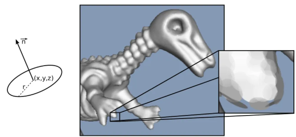
(x,y,z) r n
Figure 1.2 – The structure of a Splat (Point-based surface base element), and an example of rendering.
3. Rendering and lighting simulation provided real-time rendering of natural scenes (c.f. figure 1.1);
4. Animation and simulation focused on the dynamic aspect;
5. Streaming, our work-package, has been working on the streaming of large natural scenes.
The Streaming work-package was intended to provide a distribution frame-work for remote visualization, while participating in the Multi-model
represen-tation work-package. This double context has for example allowed us to initiate
collaboration with the team Virtual Plants from the CIRAD (Frédéric Boudon, Christophe Pradal, and Christophe Godin).
1.1.2 Streaming of Point-Based 3D Scenes
This thesis follows previous work we have done on streaming of point-based 3D scenes. A master thesis has been prepared during the period from February to June 2005. This work is described, in French, in “Mise en ligne d’environnements 3D vastes échelonnables : adaptation aux ressources et à la navigation” (Mondet,
2005)2and, in [MMG05].
This previous work was based on a client-server architecture providing inter-active walk-through of distant 3D scenes modeled as point-sampled geometry.
Point-based geometry, even if presented long ago by Marc Levoy and Turner Whitted (c.f. [LW85]), has gained recently a lot of attention from the Computer
Graphicscommunity (c.f. [RL00, KB04, Pau03, BSK04] and figure 1.2). We had
chosen point based geometry because it is inherently much more fault tolerant than meshes. To manage the points on server-side, our system was based on a Kd-Tree
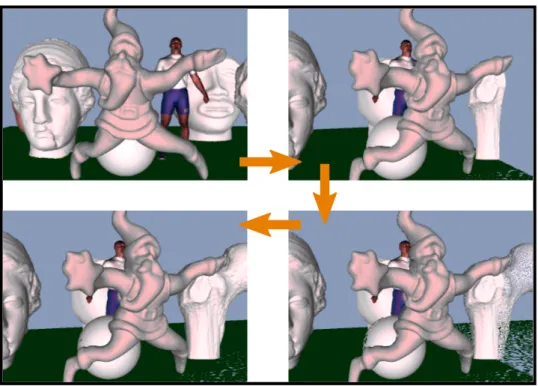
Figure 1.3 – Screenshot of the point-based streaming client with viewpoint adapta-tion.
structure representing the scene (for a complete presentation of Kd-Trees please c.f. [BKOS97]). This structure allowed us to process, on the server, viewpoint re-quests on the geometry. The server selected the visible part of the scene to send to the client (shown in figure 1.3). Regularly the client sent its viewpoint to server (if changed). The client application was based on PointShop3D’s rendering en-gine. PointShop3D is a modeling suite for point-based 3D models, developed at the EPFL [ZPKG02].
On the network, three different underlying protocols were studied:
• HTTP: the system used the apache web-server and a custom CGI-application replied to the client’s requests (the viewpoint was encoded in the URL);
• TCP: a custom TCP server was much more reactive and much less resource-greedy;
• DCCP: the protocol was still experimental: IETF3 only provided drafts of
the RFC4, and only one user-space and event-based implementation was
available.
3Internet Engineering Task Force 4Request For Comments
At the end of the master thesis, both the HTTP-based and the TCP-based were working C++ implementations of the client-server system. The DCCP-based one didn’t reach a stable state before the end of the master work.
This previous work was our first experience with 3D streaming.
1.2
Streaming of Large Natural 3D Scenes
As the NatSim project defined it, our mission is to make available 3D natural scenes for remote visualization. We aim at allowing distant users to experience interactive walk-through over the internet. Client may have heterogeneous resources, and net-work conditions may be variable.
Natural scenes have special models and structure. Specific models for plants
[Blo85], for waterways [YNBH09] or clouds [BNM+08] have been proposed. Our
goal is to keep as much as possible the botanical and physical coherency of the scene.
Next section gives some examples of application fields of our topic (section 1.2.1). Then, we provide detailed overview of the problem of 3D streaming applied to natural scenes (section 1.2.2).
1.2.1 Target Applications
The first application that motivates our work comes directly from the NatSim project. Joint Computer Science and Botanical research are setting huge datasets resulting from the simulation of the growth of forests and natural environments. The work-package in charge of the real-time rendering of natural scenes provides visualization tools for these simulated and botanically realistic environments. The specialized 3D streaming lies in between. The visualization tool should be a client application for the remote interactive visit of these scenes. The approximations needed should keep the botanical realism of the simulations.
A few botanical gardens around the world already provide some image-based
online visits. For instance, the website “Explore Kew Gardens”5proposes an
“Of-ficial Virtual Tour” of the Royal Botanic Gardens at Kew, near London. Explore
Kew Gardensmakes available 360-degrees image-based panoramas, small movies,
viewpoint narrations, maps, and text. The website is based on Flash and Java tech-nologies. A totally interactive immersion in a virtual botanic garden would be a good enhancement. Additional botanic information could be provided and, more-over, animated growth of the featured plants could be shown.
Another application of the botanical coherency are the nature-oriented educa-tional games. Such online games would, for example, propose a remote “treasure hunt” based on botanical and biological riddles.
Finally, adaptation to heterogeneous user devices could provide tools for mo-bile workers like landscape designers using Personal Digital Assistants (PDA) or
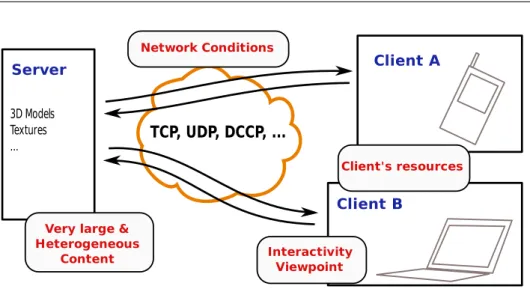
TCP, UDP, DCCP, ... 3D Models Textures ... Server Client A Client B Very large &
Heterogeneous
Content Interactivity
Viewpoint
Client's resources Network Conditions
Figure 1.4 – Main idea of a client-server system with issues raised by 3D streaming
Smart Phones. A rendering of the potential created landscape could be provided on site. Moreover it would be interesting to put in relation the virtual viewpoint (the
cameraof the rendering engine) and the actual position of the device. Such a
“Mo-bile Future Viewer” would use for example, the GPS (Global Positioning System) chip, the accelerometer and the camera which are embedded in modern PDAs and phones.
1.2.2 Issues and General Solutions
1.2.2.1 Four Main Issues
Figure 1.4 presents a simple client-server 3D streaming system. Our use case is: clients having different computing devices connect to the server to visualize a 3D scene. The server transmits it progressively. The main issues raised are shown on the figure. In the following, we detail these constraints.
Very Large Content
Natural (or non-natural) scenes may be composed of hundreds of 3D objects, and other materials (like textures). Even a single object can be large in terms of storage. For example, the geometry of the statue of David, from the Digital Michelangelo Project, represented as a mesh, consists in 2 billion polygons; even with (lossless) compression the total file size is 32 GB. Downloading completely such a model before visualizing is already completely prohibitive. Hence for 3D scenes we need accurate and progressive streaming. The sent content must not be useless (e.g. not visible) and incoming data must be decodable as soon as possible, portions of the data should lead to visual approximations of the 3D content.
Heterogeneous Client Devices
Nowadays clients of internet-based distributed applications are expected to have very heterogeneous devices. Devices like Personal Digital Assistants (PDAs) or Smart Phones are now able to render simplified 3D scenes. Graphics-hardware manufacturers now provide embedded chips with rendering capabilities, such as NVidia’s GoForce chipset which provides acceleration for 3D rendering since the “4500” model. On the other hand, small devices may even not have hardware-based floating-point arithmetic. For example the ARM architecture (Acorn RISC Machine), which is the most widely used on mobile platforms, is a 32-bit RISC CPU which only provides floating-point arithmetic as optional co-processing units with certain versions (e.g. the VFP extension). To handle these limitations on the rendering part, the Khronos Group has defined a specialized standard API for 2D
and 3D graphics on embedded systems: OpenGL ES6as a subset of the “desktop”
OpenGL API and some extensions providing easy-to-use fixed point arithmetic. Hence, we must consider that 3D streaming clients may have a wide range of de-vices, with different 3D rendering capabilities: from simple smart phones to heavy desktop computers equipped with powerful graphics cards.
Interactivity
Whatever device he is using, the client must be allowed to walk through the scene following any random path. It means that client’s viewpoint is always chang-ing and is mostly unpredictable. That is the main difference between 3D and video streaming. For 3D, even if the viewer’s position can be considered “slowly con-tinuous” (i.e. if we consider jumps in space relatively rare), a small rotation of the viewpoint may imply “kilometers” for the visible horizon. The set of visible ob-jects can change dramatically. On the other hand, the viewpoint of a video viewer has only one dimension: time. For most usages of video streaming, the viewer will see the video continuously, even if enhanced streaming systems handle the forward
and backward jumps in the video sequence as exceptional cases (c.f. [LGS+00]).
Network Conditions
The common unsafe ground of all distributed systems is the network. We con-sider the internet network of networks as our base. This means that we must handle variable conditions and no guaranteed quality of service. Bandwidth is variable and represents often a bottleneck for the application. Losses and disordering of packets are common too. A streaming system must be able to lower its requirements to provide acceptable content to the viewer, even when network conditions worsen.
1.2.2.2 One Keyword: Adaptation
There is a growing mismatch between the use of more and richer multimedia con-tent and the need to access it in an ubiquitous manner. Universal Media Access
(UMA, c.f. [MSL99]) states it nicely: provide access to advanced multimedia con-tent anywhere, anytime, and with any kind of device. Today we can only design a distributed multimedia application or produce multimedia content with hetero-geneity and context awareness in mind. Heterohetero-geneity means that we should take into account constraints that are known beforehand (devices, networks, user in-teractivity requirements). Context awareness means that a multimedia application needs to adapt, at run-time, to an evolving context (e.g. variable network condi-tions, dynamic user load on servers, geographic position of a user etc.).
Adaptation to predictable or unpredictable constraints/factors is therefore paramount in modern distributed multimedia systems. We are naturally in line with this approach, since we consider adaptation issues at every level in our 3D stream-ing system. We detail now the different aspects of Adaptation solutions for our problem.
Compression
The first solution is to transform the data, i.e. adapt the 3D scene to our needs. Since the content can be very large, and it must fit in a relatively thin pipe: the net-work bandwidth. Therefore our first goal is to represent the content as compactly as possible. Compression techniques must be used, statically or on-the-fly, to transmit smaller data over the networked channels.
Progressiveness
Another pre-processing treatment we can provide for the content is the trans-formation to a progressive (or multiresolution) representation. By progressiveness we mean that the content must be organised to be partially decodable. First portions of a progressive data-stream lead to the decoding of a coarse approximation of the modeled object (i.e. low-resolutions), and the following parts improve the quality of the approximation (i.e. higher resolutions).
Progressiveness is a key tool for multimedia adaptation. When streaming very large content, one can provide quickly a coarse resolution whose rendered repre-sentation gives visual feedback to user, while waiting for the refinements. More-over, coarse approximations of a given objects may allow the user continue the visit if the object is not of his interest; higher resolutions may not need to be transmitted at all. On the other hand, when clients use different devices in terms of memory and rendering capabilities, a streaming system must adapt the content to the device; multiresolution encodings allow to (dynamically) degrade the transmitted model to adapt them to the resources of the rendering device. Finally, progressiveness of the content allow a streaming system to adapt to the variability of network con-ditions, for example by lowering the resolution requirements when the network is congested.
Efficient packetization
From a multimedia application point of view, a transmission over the network is either a stream, i.e. an ordered sequence of bytes, if using TCP-like protocols, or a succession of unordered and potentially lost packets if using UDP-like protocols. In the former case, the peer’s operating systems hide the losses and disorderings of the underlying network to the application, but with a performance hit. In the latter case, the application has the flexibility of optimizing its performance but must man-age the losses and reorderings induced by itself. Therefore the application faces the problem of the adaptation of the transmission scheme to the loss rate of the net-work. Actually packing pieces of data in packets which have a predefined maximal size taking into account the network conditions is an adaptation problem for multi-media applications. We must hence provide efficient packetization scheme, which is aware of the characteristics of the content and of the network conditions. Pre-fetching
Interactivity, and hence the variations of the viewpoint, do not condemn 3D streaming systems designer to implement only reactive schemes. Pre-fetching is a common proactive adaptation solution in multimedia systems. It consists in trans-mitting not-yet-visible data in advance to take profit from network conditions i.e. when the bandwidth is high.
Multi-model representations
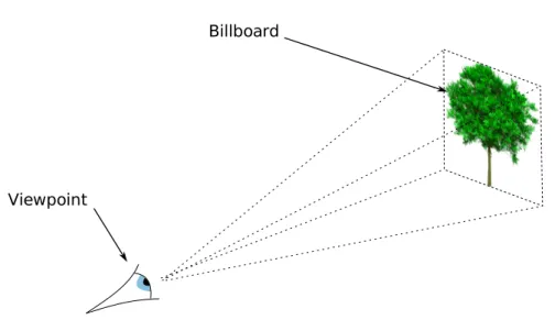
Finally, another adaptation scheme is the multi-modality of 3D objects. The idea is to have various representations of the same object, and adapt their use to the network conditions, the user’s viewpoint or its device’s capabilities. For example, a plant in a natural scene can be represented (and transmitted) as a high resolution model when viewer is inspecting it closely. But the system can choose to send only an image-based low-resolution representation (called billboard) when the viewer is far or when its rendering capabilities do not allow its device to display enough geometry.
1.3
Thesis Outline
The work exposed in this document aims at contributing to 3D streaming of natural scenes by proposing adaptation schemes following the part of the ideas described above (section 1.2.2.2). In the next chapter (2), we develop our study on a
com-pressedand progressive representation of plant models which are among the most
importantobjects in 3D natural scenes. Then in chapter 3, we present a
packetiza-tionmethod adapted to 3D multiresolution content, and we apply it to the previous
progressive model for plants. We present our work on large scenes, about adapta-tion of the system to the interactivity of the client’s viewpoint, and the 3D stream-ing test-bed we have designed (chapter 4). The chapter 5 states about the raised
issues and the learned lessons regarding the practical and implementation aspects of the work. Finally, the chapter 6 concludes and gives global perspectives about the streaming of wide natural scenes.
Progressive Representation of
Plant Models
Contents
2.1 Relevance and Specificities of Plant Models . . . 14 2.2 Representing and Modeling Plants . . . 15 2.2.1 Procedural Modeling: L-Systems . . . 15 2.2.2 Parametric and Implicit Surfaces . . . 16 2.2.3 Models for Rendering . . . 17 2.2.4 Generalized Cylinders . . . 18 2.3 A Progressive Representation of Plant Models . . . 19 2.3.1 Input Data . . . 19 2.3.1.1 Bézier-Based Generalized Cylinders . . . . 20 2.3.1.2 Our Plant Models . . . 21 2.3.2 Decorrelation Process . . . 22 2.3.2.1 Normalizing . . . 23 2.3.2.2 Grouping . . . 24 2.3.2.3 Choosing the Model Curves . . . 26 2.3.2.4 Expressing Instances and Details . . . 27 2.3.2.5 Reconstruction of the Plant . . . 28 2.3.3 Binary Coding . . . 28 2.3.3.1 Data to code . . . 28 2.3.3.2 Coding of Generic Data . . . 30 2.3.3.3 Entropy Coding of Differential Details . . . 30 2.3.3.4 A Set of Interdependent Binary Chunks . . . 34 2.3.4 Quality Metric . . . 37 2.4 Experimental Results . . . 39 2.4.1 Progressive Decoding and Grouping Policies . . . 39
2.4.2 Raw Compression . . . 41 2.5 Implementation . . . 42 2.5.1 The Encoding Process . . . 42 2.5.2 Decoding Progressively . . . 43 2.5.3 Rendering Plants . . . 44 2.6 Conclusion and Perspectives . . . 44
In this chapter, we propose a progressive compression scheme for plants based on generalized cylinders. This representation, by its multiresolution aspect, is streaming friendly. It allows us to packetize, transmit and render progressively plants with an increasing quality.
2.1
Relevance and Specificities of Plant Models
Realistic modeling of plants is crucial in NVE applications such as virtual forests or virtual botanical gardens, where users are (or will be) expected to inspect a plant closely and possibly interact with the plants they have accessed remotely.
However, realistic and detailed plant models can require up to hundreds of thousands of primitives if modeled with classical polygonal surfaces. Remolar et
al., in [RCB+02], estimated that a plant generated by XFrog, a well known plant
modeling platform1, can consist of 50,000 polygons only to represent the branches.
The plants can have 20,000 or more leaves, which themselves consist of polygons. Neubert et al., in [NFD07], reported the plant models that they used consist of up to 555,000 polygons. These numbers are for a single plant. In natural scenes, such as forests, one would expect the scene to contain a very large number of plants. The size of these plants motivates the need to stream progressively, rather than to wait until the complete plant model is received before being displayed. Progressiveness is motivated by performance constraints: the network bandwidth, but also the in-memory size, the distance of the plant to the viewpoint, etc.
Progressive representation for generic 3D objects are well studied. For in-stance, multiresolution coding of triangle meshes (c.f. [Hop96, AD01, AG05, Tau99]), point-based surfaces (c.f. [Pau03, RL00, KB04]) or hybrid representa-tions (c.f. [CN01]) are all progressive coding schemes for 3D objects. However, these representations are not suitable for plants due to the topology structure of the branches. For example, with progressive meshes, it is difficult to remove triangles above a certain level, and as a result, representation of plants by progressive meshes
does not give satisfactory results (c.f. [RCB+02]).
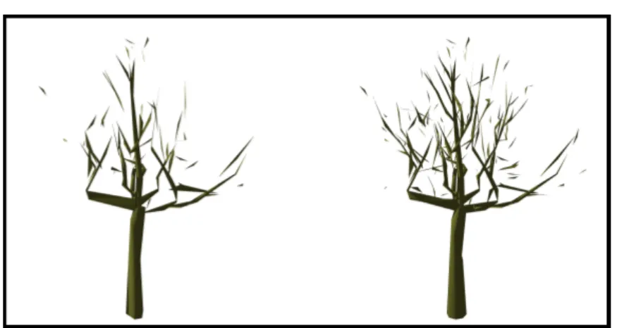
Figure 2.1 illustrates that simplification of a mesh tree does not preserve the topology, in particular the connectivity, of the tree. Hence, progressive representa-tions suited to the topology of plants are needed.
Figure 2.1 – Mesh simplification on the Walnut model (section 2.3.1.2). The original model consists of 278 632 triangles, here are presented simplified models consisting of 0.1% (left) and 0.2% (right) of the original model.
Therefore, our aim is to provide a progressive and compressed representation for plants, that preserves their botanical coherency. We want to ensure the connec-tivity between branches at each stage of decoding and, if possible, the realism of the shape of the branches regarding the plant specie.
2.2
Representing and Modeling Plants
Previous work has focussed on how to accurately model a plant (c.f. [RCB+02,
Blo85, PMKL01, PL90, NFD07]) or how to easily create a plant within the virtual
environment as proposed, for example, by the Dryad project2.
Plant geometry is particularly complex and thus motivated a variety of rep-resentations dedicated to its specific needs (c.f. [DL05, BMG06]). Branches and foliage are usually treated separately.
2.2.1 Procedural Modeling: L-Systems
From a modeling point of view, a well-known custom modeling scheme for plants are the L-Systems (c.f. figure 2.2). L-systems were introduced and developed in 1968 by the Hungarian theoretical biologist and botanist from the University of Utrecht, Aristid Lindenmayer (1925–1989). An L-system consists in a string representation of the branching structure coupled with a formal grammar (c.f. Prusinkiewicz and Lindenmayer’s book: [PL90]). The rewriting rules of the gram-mar simulate the growth of the plant. The topology and the geometry of the plant are given by a LOGO-style turtle that interprets the symbols of the string as ometric commands (c.f. [Pru86, FKMP03]). We note that, in this system, the
Axiom: X Rule: F=FF;X=F-[[X]+X]+F[+FX]-X Axiom: FF Rule: F=FF[+F--F][-F-F] Axiom: F Rule: F=F-F++F-F
Figure 2.2 – Examples of Basic 2D L-Systems (Generated with Inkscape).
ometry of a symbol is built according to the geometry of previous elements, and leaves are instances at different places of the same geometric symbol.
2.2.2 Parametric and Implicit Surfaces
The previous idea has inspired a lot of work (our progressive representation stands among of them). More generally, some high level representations for branches have been proposed based on parametric (c.f. [Blo85]) or implicit surfaces (c.f. [GMW04]). They rely on a skeleton of branches which is extended with radius (given by cross sections or implicit functions). The skeleton is defined as a set of connected parametric curves. These topological structure representations have the advantage of being compact compared to more discrete representations such as mesh and provide support for animation (which is not the case of the simplified models whose connectivity is lost in figure 2.1). By default, however, they are not
Viewpoint
Billboard
Figure 2.3 – An example of billboard: A pre-rendered image, presented as an impos-tor in front of the viewpoint (generally, a billboard is a texture sticked on a rectangular piece of mesh).
adapted for progressive description. Our goal in this chapter is precisely to fill this gap.
2.2.3 Models for Rendering
From a rendering point of view, some representations are based on billboards i.e.
pre-rendered images used as impostors, c.f. [MNP01, DN04, BCF+05]; see also
figure 2.3. Also representations based on points (c.f. [WP95, DCSD02]) or
poly-gons (c.f. [RCB+02, ZBJ06]) have proposed adaptive schemes for displaying trees.
These representations mainly focus on foliage (leaves) and thus can be seen as complementary to ours since they are usually complemented with polygonal rep-resentations of trunk and branches. If these reprep-resentations offer some interesting results, they usually require a large amount of data, in particular with points and im-ages. Polygonal representations on sparse geometry such as foliage are not totally convincing. These representations can be streamed with classic methods since they use classic primitives with low-level abstraction. By default, however, they seem more dedicated to static representations. Additionally, they have to be attached to a skeleton representation to support animation.
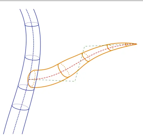
Figure 2.4 – Generalized Cylinder with Radius along the branch.
2.2.4 Generalized Cylinders
On the other hand, Generalized Cylinders are a representation focusing on the branching structure of the plant, i.e. “skeletal-based” (c.f. [Blo85]). A branch is rep-resented by an axis curve, a parametric curve defined by a set of control points, and parameters defined along the branches (c.f. figure 2.4). Such generic high level rep-resentation can then be displayed as generalized cylinders (c.f. [Blo85, PMKL01]) or implicit surface (c.f. [GMW04]) and is much more compact than a mesh rep-resentation. For example, the Walnut (presented in section 2.3.1.2) at full resolu-tion only requires about 10 772 control points using generalized cylinders com-pared to 278 632 triangles using a mesh model. Recent work has also studied the real-time rendering of generalized cylinders using modern graphics hardware (c.f. [GM03, BW05]). Additionally, this representation, which is based on a skeleton structure, can possibly be extended with kinetic informations for use in animation. The branches are organized inside a n-ary tree data structure modeling the struc-ture of the plant. We call such a data strucstruc-ture a n-tree, to avoid confusion with the concrete plant object we are actually modeling. This representation has been chosen as a starting point for our work (see also [Bou04]).
Decorrelation
models instances detail vectors
entropic coder Huffman Coder builder Binary coding HuffmanCoding
Plant
(branching system)
Set of Binary Chunks
Figure 2.5 – The encoding process for a model based on skeletal representation.
2.3
A Progressive Representation of Plant Models
In this section, we detail the development of our streaming-friendly representation and coding of plant models based on generalized cylinders. This work has been
first published in the paper [MCM+08] and then extended in [MCM+09].
Figure 2.5 outlines the steps from encoding to streaming of our representation, and guide the presentation of this section. Our starting point is a natural scene using plant models based on precise skeletal representation (section 2.3.1). This representation served as the basis for our proposed compressed, progressive repre-sentation that decorrelates information into three components called branch mod-els, instances, and detail vectors (section 2.3.2). The detail vectors are compressed with entropy coding and other pieces of data are efficiently coded (section 2.3.3), resulting in a set of binary chunks. Finally, each chunk is assigned an importance value, which is then used for scheduling the chunks in the progressive decoding stream (section 2.3.4).
2.3.1 Input Data
As a starting point, in this section, we aim at providing a good understanding of what we consider as our input data. First, we describe precisely the generalized cylinder with a data-structure viewpoint (section 2.3.1.1). And then we present the actual plant models we have used for testing, evaluating and experimenting the methods presented in this chapter (section 2.3.1.2).
other control points Parent Branch
first control point Attach Parameter Bézier Curve Control points Bézier Curve Radius (r)
Parameter on branch (u)
Geometry of a Bézier branch Radius profile of a branch
0 1
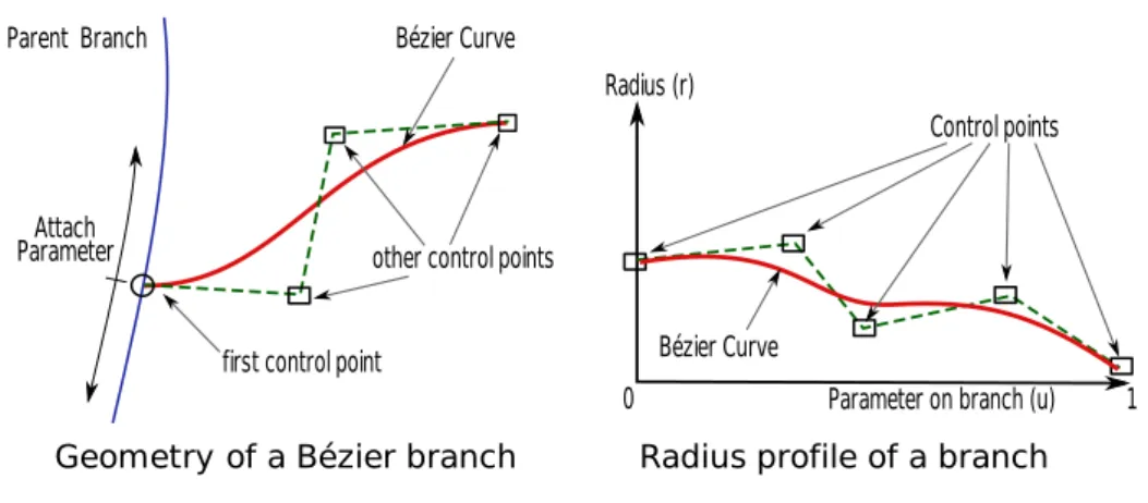
Figure 2.6 – On the left, the Bézier curve representing a branch with its attachment parameter (u) on its parent branch. On the right, the Bézier curve representing the radius along a branch (i.e. (u, r) ∈ [0, 1] × [0, ∞]).
2.3.1.1 Bézier-Based Generalized Cylinders
Our representation focuses on the branching structure of a plant and is thus based on a skeletal representation. Each branch is a generalized cylinder: an axis curve,
which is a 3D Bézier curve defined by its control points3 and axial parameters
such as the radius, color or texture coordinates modeled as Bézier curves along the branch. In practice, we use for now only radii as axial parameters, defined by 2D Bézier curves. As presented in section 2.2, we render and display this high level representation as 3D generalized cylinders (c.f. [Blo85, PMKL01]).
The branches are organized inside an n-ary tree data structure giving the struc-ture of the plant. The root of the n-tree is the trunk of the plant and branches borne by the trunk are the n-tree children of this trunk. Each child branch contains a
at-tachment parameter(u ∈ [0,1]) giving the position of the attachment point on its
bearing parent branch (as in [PMKL01]). The parameter u defines the first control point of the Bézier curve of the child branch. The remaining control points are encoded in the child branch by their three coordinates in space.
Axial parameters are also defined thanks to the attachment parameter u. We take the example of the radius but the scheme can be adapted to textures or colors. The case of the radius of the branch illustrates how attributes along the branch are coded. A radius is defined as a positive real value along the branch. To model it as a smooth function along the branch, we represent its values as a series of control
points (ui, ri) of a Bézier curve of degree m, where (ui)i=0. . . m is an increasing
sequence in the interval [0,1] that defines the location of the branch, and (ri)i=0. . . m
characterizes the radius for the corresponding given location. Note that the degree of the radius curve is not related to the degree of its bearing branch.
Figure 2.6 summarizes the structure of the model.
Figure 2.7 – The Walnut model (digitized by Sinoquet et al. c.f. [SRG97])
2.3.1.2 Our Plant Models
Compression and streaming have been applied to two real plants. We have used two digitized plant models: a 20 year old Walnut tree (from [SRG97]) and an apple tree (from [CSKG03]). The walnut tree is 7.5m high and 5.8m wide (c.f. figure 2.7). It took two weeks to digitize using a Polhemus 3Space Fastrack electromagnetic device. We pre-processed it by fitting Bézier curves to a series of digitized points representing branches. Our representation is thus composed of approximatively 1900 branches with 6900 control points for the branches and 5800 control points
Grouping Normalisation
Model Branch (average) Instantiation
Parameters
Differential Details
...
Figure 2.8 – Overview of the decorrelation process.
for the radii. The apple tree is 6 year old, 2.8m high and 2m wide and is made of 430 branches, 1350 control points for the branches and 1100 for the radii.
To extend our experimental range of models, we have also generated some examples using L-systems (c.f. [PL90]). For example, we used here a fir-like tree composed of 6 945 branches, 208 354 control points for the branches and 13 900 control points for the radii. Of course, if used in an application, L-systems models would have been surely more efficiently coded and transmitted by sending their generative rules and parameters. But determining generative process of a given tree is not always possible, in particular for measured tree.
2.3.2 Decorrelation Process
To encode a plant as a compressed multiresolution representation, we exploit the similarity of the Bézier curves representing the branches and the radii separately. The idea of the compression algorithm is to replace the absolute coding of most control points by differences compared to a small set of average Bézier curves. We group the branches and the radii independently to profit from the similarity inside each group of Bézier curves, in order to make these differences be small. Therefore they may be coded with a fewer bits, leading to a compact coding.
A simplified overview of this decorrelation process is shown in figure 2.8 for the case of Bézier curves representing branches (the process for radii is equiva-lent but less visual). First, we process a normalization transformation to make the Bézier curves comparable (section 2.3.2.1). Then we group the curves following similarity criteria (section 2.3.2.2). And for each group, we extract a model Bézier curve, i.e. a curve which best represents the curves of the group (section 2.3.2.3). This model curve allows us to express the Bézier curves of the group as two entities:
Set Of Bézier Curves Groups Of Bézier Curves Degree Reduction Degree-Based Grouping Hierarchical Clustering Scale Based 2D Grid Based Normalization Transformation
Figure 2.9 – The process of normalizing and grouping Bézier curves seen as cascad-ing filters. All filters work on generic Bézier curves except the normalization trans-formationwhich has two versions, one for branches and one for radii.
Degree
Reduction DegreeRaising
Figure 2.10 – Degree reduction and raising of a 2D Bézier curve. The original curve has degree 5 (6 points), its degree is lowered to 2 and elevated back to 5.
parameters and allow the decoder to instantiate the model bézier curves to build approximated branches and radii and place them on the tree. The details are the differences between the actual curves and the model one, details allow the decoder to deform the model curve and rebuild the original one.
2.3.2.1 Normalizing
In order to compare and to code differences between two branches, a so called
standard representationof the Bézier curves is necessary. This normalization is
based on two steps. The first one is optional but applicable to every Bézier curve which has a degree greater than 2. The second one, while mandatory, is different for branches and radii to profit from their particular geometric properties. Figure 2.9 (left) shows how those steps are chained as filters.
Optional Degree Reduction
To have Bézier curves be comparable by their control points, and release the constraint on grouping according to the degree, i.e. according to the number of
Z X y Transformation P(u) P1 P2 P3 P4 P5 (0,0,1) (0,0,0) Z X y (0,0,1) (0,0,0) P'1 P'2 P'3 P'4
Figure 2.11 – Main idea of the normalization transformation for branches.
control points (c.f. next section 2.3.2.2 and [MCM+08, MCM+09]), we can build
the standard representation by preprocessing the curve: we use a degree reduction algorithm (c.f. figure 2.10). In practice, any Bézier curve of degree bigger than 2 is approximated by a curve of degree 2. We apply the algorithm called “CEQ 2” from [BWX95] which is based on Constrained Equioscillation and has the convenient property of interpolating the endpoints of the approximated curve.
Transformation of Branches
We make all branches comparable thanks to an affine transformation converts back and forth between an original branch and its standard form. The affine trans-formation is defined so that the first and last control points of the original Bézier curve, map to the origin (0,0,0) and the point (0,0,1) respectively (c.f. figure 2.11). We characterize this first mapping by a translation, two rotation angles, and a uniform scaling factor. Since we choose to apply a uniform scaling, there is a remaining degree of freedom, which corresponds to another rotation around the z axis. To completely define the affine transformation, we fix the rotation around the z axis so that the center of gravity (or average) of the control points, lies in the (x,z) half-plane. In the case of degree 2 curves, which have only one free point (the two other points have been fixed to (0,0,0) and (0,0,1)), this latest rotation brings all curves totally in the same half-plane.
Transformation of Radii
Since the parameters uialready fall in the interval [0,1], we normalize the
fam-ily riby dividing it by the average norm of the radii. All normalized radii profiles
provide hence the same average thickness.
2.3.2.2 Grouping
The grouping of branches is a step in the decorrelation process which impacts the performance whole scheme. The accuracy of the approximation by model Bézier curves as well as the performances of the entropy coding of the detail vectors may depend on the quality of the grouping.
Grouping is a global function that partitions a set of normalized Bézier curves in a set of groups of normalized Bézier curves. This function can be seen as a cas-cade of filters, i.e. grouping algorithms. We have implemented several grouping filters, each to satisfy different criteria: compression efficiency, quantization error minimization, or the visual aspect of the progressive decoding. Note that these cri-teria apply for both the original (full resolution) plant and the intermediate, partially rendered, plants. Figure 2.9 (right) shows how we can combine those grouping fil-ters. The following details the grouping schemes we have implemented.
Degree-Based Grouping
The first grouping strategy we have successfully implemented is simply based
on the degree of the Bézier curves (c.f. [MCM+08]). The degree of a Bézier curve is
its number of control points less one, hence, we just group the curves according to their number of control points. This approach, even if apparently straight forward, allows us to compare the curves without having to elevate their degree (elevating the degree of a Bézier curve adds points but does not add “information”). Moreover, as shown in figure 2.9, we still use this grouping algorithm in all cases. But we must note that, if we use the optional degree reduction step of the normalization presented in previous section (2.3.2.1), this grouping filter only partitions in two groups: the curves of degree 1 and those of degree 2. As mentioned before, the goal of the degree reduction pass, was rightly to remove the constrain of the degree on the groups.
Hierarchical Clustering
In order to minimize the quantization error (c.f. section 2.3.3.3), we add a grouping filter based on a hierarchical clustering algorithm [Joh67]. Clustering is applied on the Bézier curves by first defining an initial distance between every two curves. Then, a greedy procedure merges the clusters two by two, choosing, at each step, the smallest distance until the desired number of clusters is reached. At each merge, the distances to the newly created cluster are easily computed using a link function, which computes the distance to the new cluster from the distances to the two original clusters. The algorithm ends thanks to a stop condition based on a target number of clusters and/or a minimal radius of cluster.
The functions used as distance and link function have significant impact on the resulting groups. After trying several combinations, we have converged to the most natural ones given our goal. As distance we use the sum of the norms of the differences between control points; as link function we choose to compute the average distance weighted by the number of curves in the clusters. Those choices are natural, as the differences between control points will be used to compute detail vectors (c.f. section 2.3.2.4), and the model curves will be computed as an average curve of the group (c.f. section 2.3.2.3).
Scale-Based Grouping
An additional grouping strategy, called scale-based, uses the length of the branch or the average of the radius (both are equivalently obtained from the scal-ing factor of their respective normalized representation) to create the groups. We partition uniformly the segment defined by the minimal and maximal lengths (or scales) in a target number of segments. We then create the groups by associating the curves with segments.
This grouping filter has been specially designed for Bézier curves representing branches (even if it is usable for radii). As a typical tree has fewer long branches and more short branches, longer branches tend to be grouped in smaller groups, while shorter branches are grouped into bigger groups. Since short branches are likely not to bear children branches, having a less accurate version of these branches in the intermediate tree is visually acceptable. For long branches, the shape of a branch affects all children branches and the whole shape of the tree, they also cause popping effects. Such scale-based grouping not only preserves good compression, but gives better visual results for the progressiveness of the tree (c.f. section 2.4.1).
2D Grid-Based Grouping
Finally, another grouping strategy specialized for Bézier curves of degree 2 which represent branches has been implemented. This filter uses the geometric position of the middle control point of the approximating degree 2 Bézier curve. It is based on a two-dimensional grid partitioning of the (x,z) plane, taking advantage of the fact that the normalization transformation has brought the middle point in that plane (last rotation). For other degrees, or for the radii, we can use the average of the control points to process this kind of grouping. This ensures compatibility for all kinds of Bézier curves but has little less heuristic sense.
The Best Compromise
In section 2.4.1, we present some experiments on the grouping policies. These experiments lead us to choose a best compromise setup, which consists in using the degree reduction option for both branches and radii, and grouping only the branches using the scale-based filter (creating four groups). Obviously our choice can be challenged: other performance criteria or other experimental data (plant models) may produce a different best compromise. Nevertheless, we are using this
best compromise setup for the rest of the experiments for the sake of simplicity.
Moreover, changes in grouping strategy induce small quantitative changes, they do not perturb qualitative observations on the results.
2.3.2.3 Choosing the Model Curves
The previous process has allowed us to obtain a set of groups containing normal-ized representations of the Bézier curves. We can now compute the model curve
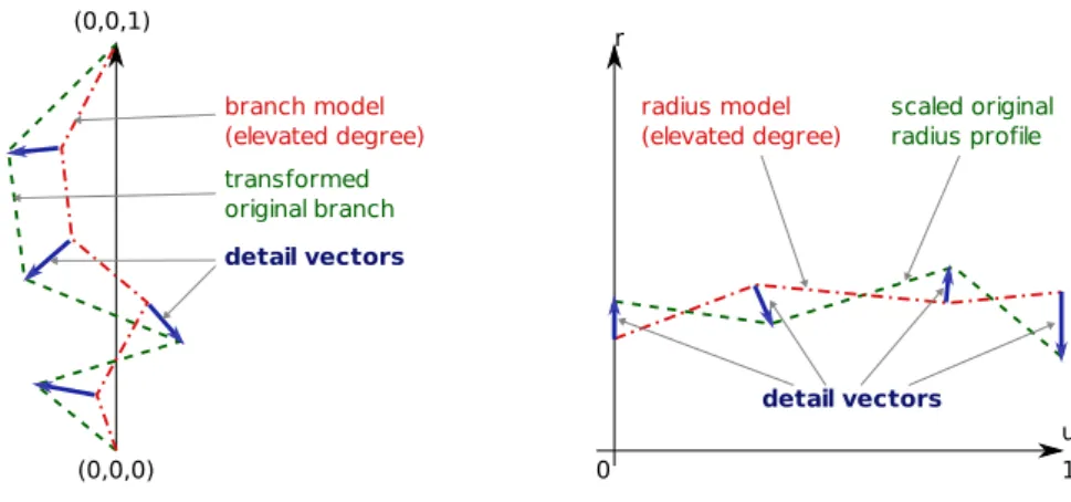
P(u) P1 P2 P3 P4 P5 Z (0,0,0) (0,0,1) branch model (elevated degree) transformed original branch detail vectors r u 1 0 radius model
(elevated degree) scaled originalradius profile
detail vectors
Figure 2.12 – Definition of the detail vectors for branches (left) and radii (right). In green regular dash, an original curve after normalization transformation, and in red irregular dash, the model curve of its group after optional degree re-elevation. The detail vectors(blue) are the difference vectors between the control points of the nor-malized original curve, and their corresponding control points on the average curve.
for each group as an average of the other curves. The average Bézier curve has the same common degree of the group (and in the case of branches, its endpoints are also (0,0,0) and (0,0,1)). Control points are computed such that the i-th control point of the average curve is the barycenter of the i-th control points of the curves of the group.
2.3.2.4 Expressing Instances and Details
For each branch or radius in a group, we now code in differential form the corre-sponding Bézier curve relatively to the model curve, storing, instead of the coor-dinates of the control points, their differences to the corresponding control point of the model curve (c.f. figure 2.12). We call those differences detail vectors. If
degree reductionhas been used for normalization, we re-elevate the degree of the
model curve before computing the detail vectors. Degree raising is a deterministic algorithm (c.f. [Far02] and figure 2.10), it can be therefore used both on encoder and decoder side, and provide the same result.
For each curve, we can also define instantiation parameters. They are the min-imal requirements which will allow the decoder to draw a generalized cylinder from the branch and radius models on the partially rendered tree, i.e. to place it on a parent branch cylinder. For branches we need:
• a reference to the model branch; • a reference to the parent branch; • the attachment parameter (u);
For radii the case is simpler, the requirements are: • a reference to the model radius;
• the scaling factor used during normalization.
All those parameters define what we call instances in our modeling scheme. The encoding of a branch cylinder is now defined by five entities: the branch model, the radius model, the instantiation parameters, the branch details and the radius details. Next section explains how the original tree is reconstructed.
2.3.2.5 Reconstruction of the Plant
Our representation allows branches of a plant to be displayed progressively as gen-eralized cylinders in two ways. First, the models are transformed thanks to the in-stantiation parameters; the resulting instances are displayed attached to their parent branch, showing an approximate cylinder of the branch. Second, the detail vectors may refine the shape of the branch previously rendered.
The approximation of a Bézier curve is built by applying the inverse of the nor-malization transformation to the model curve. However, algorithmic modifications may be applied to the approximated curve to improve its visual aspect.
Determin-isticmodifications do not change the accuracy of the cylinder with respect to the
original one just its rendering result. For example, temporary approximations of the radii profiles (while details are not available or decoded) can be made more pleasant looking just by bounding the radius for u = 1.
2.3.3 Binary Coding
After transforming our set of connected Bézier cylinders into a progressive repre-sentation, we obtain three classes of data: models, instances and details. We now efficiently code them to build a set of interdependent pieces of data, called binary chunks. Some general information, necessary for the decoder, will be agglomerated into an unclassified chunk of data: the header.
In this section, we first detail and classify the pieces of data we actually have to code (section 2.3.3.1). Then we focus on the “low-level” coding: first of the generic pieces of data such as numbers and vectors (section 2.3.3.2), and then of the detail vectors which deserve entropy coding (section 2.3.3.3). We finally assess the three classes of binary chunks we obtain after coding (section 2.3.3.4).
2.3.3.1 Data to code
For the main classes of data, we express here which parameters have to be coded to be able to progressively decode a plant.
The Models
First, for the branch curves, it is important to note that since the models are in normalized form, the first and last control points do not need to be coded. Those are always (0,0,0) and (0,0,1). For example, Bézier curves of degree 4 representing branches only need 3 intermediate points to be defined. Moreover, if we have used the degree reduction option, a branch model can only be of degree 1 or 2, therefore only 0 or 1 control points need to be coded (this leads to improvements in the compression ration, c.f. section 2.4).
To reference both the branch model and radius model while decoding an in-stance, we need to define a model identifier; a positive integer strictly smaller than the total number of models.
Hence, a branch model of degree d consists in d - 1 3D control points and one “model identifier”. Whereas a radius model of degree m consist in m + 1 2D control points and one “model identifier”.
The Instances
To instantiate a model branch on the progressively decoded tree, we first need to reference its parent branch, which is another instance. This requires coding of an instance identifier and a reference to another instance. Both identifiers are also bounded integers. Then to place the curve on its parent branch, we need the attach-ment parameter, which is a bounded real number (u ∈ [0,1]).
Then we need to transform the model curve of the branch. For that, as shown previously, we need first to reference the branch model of the instance by its model identifier. Then we need the normalization transformation. As seen in sec-tion 2.3.2.1, the normalizasec-tion is the composisec-tion of one translasec-tion, one scaling and three rotations. However, thanks to the attachment parameter we can have the position of the first control point of the curve. We know one point, which is (0,0,0), and its corresponding translated point, given by the parent branch and the attach-ment parameter. Therefore we do not need to code the translation; we can obtain it from data which is already decoded. The remaining transformation parameters are three scalars for the angles of rotation and a scalar for the uniform scaling.
For the radius, we just need to code a radius model identifier and one scaling factor to transform the radius model to the right approximation.
The Details
As for the models branches, differential details for curves of degree d require the coding of d - 1 3D vectors as they are differences between normalized branches. Moreover, to reference the branch to whom the details belong, we need to join an instance identifier.
Similarly, details vectors for Bézier curves representing radii of degree m, con-sist in m + 1 2D vectors and one “radius model identifier”.
We choose to “pack” together, in the same binary chunk, shape differences and radius differences of a given branch. Evaluation of the case when details are treated
separately is left for future work but we must note that the only direct overhead would be to have to code an additional instance identifier in the Radius Detail Vectors binary chunk.
2.3.3.2 Coding of Generic Data
Excluding the detail vectors, which will be studied in the next section, we only have three types of numbers to code: general scalars, bounded scalars and bounded integers.
• General scalars are coded with floating point representation as we do not have information on them; they can be arbitrarily big or small. Floating point is, for us, the safe “default” encoding, when we do not know enough about the number. They are the control points of the model Bézier curves and the scaling factors of the instances (one for the branch and one for the radius). For example, to remain “compatible” with strangely formed trees (with ar-bitrarily big ratios between small and big branches), we can not asume any-thing on scale factors; a scale of 0.1 is very different both from 0.0001 and from 1000.
• The attachment parameters and the rotation angles, have the particularity of being bounded and uniformly spread in between their bounds. Hence, as the bounding intervals of those scalars can be uniformly sampled, they can be serialized more efficiently with fixed point arithmetic. A binary integer can represent the ratio (∈ [0,1]) regarding the bounding interval. Therefore, we have to choose, for each parameter the precision, i.e. the number of bits used to code the number.
• Finally, bounded integers, such as identifiers and references, can be coded
using a limited number of bits: ceil(log2(MaxId))where MaxId is the
maxi-mal number to code. Identifiers are regularly ordered from 0 to the number of identifiers to code, therefore this coding is optimal (i.e. the maximal number to code is the number of identifiers less one).
2.3.3.3 Entropy Coding of Differential Details
One advantage of multiresolution differential coding is that the induced differences are small, very correlated (see for instance figure 2.13). This provides the ability (i) to quantize small detail vectors with a small number of bits, and (ii) to choose accurate binary representative symbols according to their distribution. In this sec-tion, we first present our quantization method, then we show that the evaluation of our resulting detail vectors leads to a beneficial usage of an entropy coder.
To evaluate the accuracy of using an entropy coder in our method, we have computed, for a given quantization (i.e. a given number of bits per floating point number), the induced error and the theoretical entropy of the represented data. The
-1 -0.5 0 0.5 1 1.5 2 2.5 3-0.8-0.6 -0.4-0.2 0 0.2 0.40.6 0.8 1 1.2 -3 -2 -10 1 2 3 4
Figure 2.13 – Distribution of the detail vectors for the branches of the Walnut, using our best compromise set up.
maximal induced error gives the accuracy of the quantization, while the computed theoretical entropy gives the mean number of bits to expect after Huffman coding. Quantization
The quantization can be vector or scalar. We have carried out experiments with
both methods. Our first results were using vector quantization (c.f. [MCM+08]).
The vector quantization is carried out in two steps. First we compute the AABB (Axis-Aligned Bounding Box) of all detail vectors (by finding the min and max of the x,y,z coordinates). Then, to quantize each coordinate into bpc bits (Bits Per
Coordinate), we build a 3D grid corresponding to 23· bpc vectors uniformly
dis-tributed in the AABB. Each detail vector is then represented by the symbol of the nearest of the vectors discretized on the grid. The quantization error is thus the distance from the quantized vector to the original detail vector. To reconstruct the quantized vectors, a header containing the AABB of the vectors (6 floating point numbers) and the number of bits per coordinate is sufficient.
The resulting error for a given number of bits per coordinate could still be decreased by processing a few iterations of a classification algorithm such as k-means. However, the resulted gain would be offset by increased header size, since transmission of the actual values of the representing symbols chosen by the classi-fication would be necessary. We let the evaluation of the tradeof between the header size and the accuracy of the algorithm for future work, it is likely to become useful when implementing forest-based compression (c.f. 2.6), since the same header will be shared by different trees in the forest.

![Figure 2.7 – The Walnut model (digitized by Sinoquet et al. c.f. [SRG97])](https://thumb-eu.123doks.com/thumbv2/123doknet/3718187.110958/39.892.215.754.169.802/figure-walnut-model-digitized-sinoquet-et-al-srg.webp)