HOUSEHOLD SURVEYS AS A SOURCE OF DATA FOR EVENT HISTORY
ANALYSIS. THE STUDY OF FAMILY RELATED LIFE EVENTS IN ARGENTINA USING THE ENCUESTA PERMANENTE DE HOGARES Benoît LAPLANTE, María Marta SANTILLÁN and María Constanza STREET 0B
INRS
1BUrbanisation, Culture et Société
JANUARY 2008Household surveys as a source of data for
event history analysis. The study of family
related life events in Argentina using the
Encuesta Permanente de Hogares
Benoît LAPLANTE, María Marta SANTILLÁN and María Constanza STREET
Institut national de la recherche scientifique Urbanisation, Culture et Société
Benoît Laplante
benoit.laplante@ucs.inrs.ca María Marta Santillán
Universidad Nacional de Córdoba (Argentina)
mm_santillan@yahoo.com.ar
María Constanza Street
constanza.street@ucs.inrs.ca
Inédits, collection dirigée par Mario Polèse :
mario.polese@ucs.inrs.ca
Institut national de la recherche scientifique Urbanisation, Culture et Société
385, rue Sherbrooke Est Montréal (Québec) H2X 1E3 Téléphone : (514) 499-4000 Télécopieur : (514) 499-4065
www.ucs.inrs.ca
TABLE OF CONTENT
List of Tables ... iv
RÉSUMÉ/ABSTRACT ... V INTRODUCTION ... 1
1. THE EPH, ITS DESIGN AND THE POSSIBILITIES IT OFFERS FOR EVENT HISTORY ANALYSIS ... 1
2. TWO FAMILY RELATED LIFE EVENTS ... 3
2.1 The effect of demographic and socioeconomic factors on the hazard of becoming poor in Argentina ... 3
2.2 From consensual union to matrimony ... 6
3. MODEL ... 11
4. RESULTS ... 15
4.1 The effect of demographic and socioeconomic factors on the hazard of becoming poor in Argentina ... 15
4.2 From consensual union to matrimony ... 19
5. LIMITS AND DISCUSSION ... 25
iv
List of Tables
Table 1 Effect of demographic characteristics on the hazard of becoming poor
(Poisson regression) (Models 1 to 7) ... 15
Table 2 Effect of demographic characteristics on the hazard of becoming poor
(Poisson regression) (Models 8 to 11) ... 16
Table 3 Effect of birth on the hazard of becoming poor (Poisson regression) ... 17
Table 4 Effect of union dissolution on the hazard of becoming poor (Poisson regression) . 18
Table 5 Effect of some socioeconomic characteristics on the hazard on converting a
consensual union into marriage (Poisson regression) (Models 1 to 10) ... 20
Table 6 Effect of some socioeconomic characteristics on the hazard on converting a
consensual union into marriage (Poisson regression) (Models 11 to 17) ... 20
Table 7 Effect of pregnancy and birth on the hazard on converting a consensual union into marriage (Poisson regression) ... 22
RÉSUMÉ/ABSTRACT
L’analyse des transitions, ou analyse des biographies, est une méthode couramment utilisée pour étudier les événements démographiques qui surviennent dans les familles et les ménages, mais son usage est limité par la rareté des enquêtes biographiques. Les auteurs proposent une méthode qui permet de réaliser des analyses analogues à celles que l’on associe habituellement à l’analyse des biographies à partir des données recueillies par les enquêtes auprès des ménages qui utilisent des panels rotatifs. Ils illustrent cette méthode en utilisant les données de la Encuesta Permanente de Hogares argentine pour étudier deux événements importants dans la vie des familles : devenir pauvre et transformer une union libre en mariage.
Mots-clés : Analyse des transitions; Analyse des biographies; Familles; Ménage; Pauvreté; Coabitation; Mariage; Argentine.
Event history analysis is an important tool in the study of families and households, but its use is complicated by a lack of availability and difficulty in obtaining true biographical survey data. The authors argue that the data gathered by multi-purpose prospective surveys, such as those which use rotating panels for sampling efficiency, can be used to perform analyses very similar to event history analysis. They demonstrate how this can be done, using data from the Argentinean Encuesta Permanente de Hogares in the study of two family related life events: becoming poor and turning a cohabiting union into a marriage.
Keywords: Event history analysis; Family studies; Household; Poverty; Cohabitation; Marriage; Argentina.
INTRODUCTION
Event history analysis can play an important role in the study of families and households, but its use is complicated by a lack of availability and difficulty in obtaining true biographical survey data; that is, complete sequences of life events and the time at which they occurred recorded for a complete sample of individuals, either through retrospective surveys or through panel or repeated measurement surveys in which the sample is observed from its point of origin with respect to events.
Along with the census, multi-purpose prospective surveys are the “back-bone” of national statistical systems. These surveys gather various types of data on the population (family income and spending, unemployment, etc.). Several of them use some form of panel design, such as rotating panels, but do so for sampling efficiency than with the objective of gathering longitudinal data. However, even without the intention of gathering longitudinal data, multi-purpose surveys that use panel design do actually gather longitudinal data which, at the very least, measure some relevant characteristics repeatedly over some period and this allow to observe some changes. From the perspective of conventional wisdom, such data are not well suited for event history analysis. We argue that despite their limitation, they may be used to study life events in a way very similar to event history analysis. It is the purpose of this article to demonstrate how this can be done, using data from the Argentinean Encuesta Permanente de Hogares in the study of two family related life events: becoming poor and turning a cohabiting union into a marriage.
1. THE EPH, ITS DESIGN AND THE POSSIBILITIES IT OFFERS FOR EVENT HISTORY ANALYSIS
The Encuesta Permanente de Hogares (EPH, “Permanent Survey of Households”) is a multi-purpose survey realized by the Instituto Nacional de Estadística y Censos (INDEC), the national statistical agency of Argentina. It has been conducted since 1973 in the major urban centres of the country and has been progressively extended so as to cover all urban centres and about 70% of the population of the country. The main purpose of the EPH is to gather information on socio-demographic characteristics, labour force participation, income and wealth distribution. The information gathered through the EPH is primarily used to estimate activity rates and unemployment rates as well as the proportion of households that are below the poverty line. The rotating panel design of the EPH allows the monitoring of households for up to a maximum of three observations periods over 18 months. Because of its use of a rotating panel design, the EPH is the only source of data survey maintained by the INDEC that can be used for longitudinal analysis.
The EPH is a sample-based survey, where the questionnaire is administered to a probabilistic sample representative of the population;1 in May 2003, the sample included 30,473 households and 92,294 individuals. Up until the beginning of 2003, the survey was conducted twice a year, in May and October, using a rotating panel design in which one fourth of the sample was renewed every time the survey was conducted. Under that design, every household included in the sample remained in it for a period of up to 18 months during which it was interviewed up to four times. For convenience, each realisation of the survey is referred to as a wave.
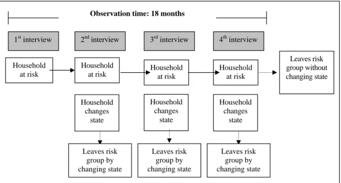
From the perspective of event history analysis, households, or their members, in some state of interest (v.g. above the poverty line or living in a cohabiting union) at the time they are interviewed for the first time are at risk of leaving that state and entering another (v.g. falling below the poverty line or turning their union into a marriage) and are observed of being at such risk from the time their enter the sample through the time they either leave their state of origin or leave the sample without leaving their state of origin. The rotating panel design of the EPH thus allows registering events of interest as they occur. As in a conventional event history analysis setting, the households or individuals leave the risk group either by changing state or by leaving the sample without having changed state if they haven’t done so by the time of the fourth interview (Figure 1).
1
In the EPH, a household is defined as a person or group of persons related or not, who live under a same roof and share the costs of food or other basic necessities. The random sampling of households is done in two steps: 1) subdivisions are selected from each region of the country where the survey is conducted; 2) a list of dwellings for different areas is drawn-up and a second random selection is carried out. The households located in these dwellings are the ones surveyed (INDEC, 2003).
2
Figure 1. Selection of the EPH observation units.
Given that the EPH records the current value of its variables at each wave, it provides the information needed to build time-varying independent variables. This is obviously the case for time-varying independent variables that are thought of as series of current values of a given variable that is known to change over time (e.g. size of the household, total household income), but it is also true for time-varying independent variables that are themselves defined as changes of state or events, for example the birth of a child. Such variables can be built by comparing the values of the relevant recorded variable from one wave to the next. In theory, the type of analysis we are describing could be done for any period of time since the time the survey was initiated. However, the EPH database available to researchers does not provide the information required to link the data collected from the household from one wave to the next before May 1995. Furthermore, the rotating panel design of the survey has been modified after the May 2003 wave; since then, the EPH still uses a form of rotating panel design but in such a way that households are interviewed four times over a 18 months period, with a two trimester gap between the second and the third interview. The design has been altered in a manner that makes it impossible to link the data collected from households which were in the sample before and after the implementation of the new design (INDEC, 2003: 16-19). As a consequence, longitudinal analyses can only be performed for the period ranging from May 1995 to May 2003, or from January 2003 to the present. In this article, we use data from the former period.
Household at risk
Household
at risk Household at risk Household at risk
Household changes state Leaves risk group by changing state
1st interview 2nd interview 3rd interview 4th interview
Observation time: 18 months
Household changes state Leaves risk group by changing state Leaves risk group by changing state Household changes state Leaves risk group without changing state
2. TWO FAMILY RELATED LIFE EVENTS
2.1 The effect of demographic and socioeconomic factors on the hazard of becoming poor in Argentina
During the 1990s, Argentina has seen the incidence of poverty significantly increase. While in 1993, 16.8% of the population was considered to be living below the poverty line, at the beginning of 2003, this number had risen to 51.3%.2 This increase has not only meant a deterioration in living conditions compared to other Latin American countries, but also a significant decline compared to the situation observed in the country during previous decades; considering that in 1980 the percentage of the population considered as poor was 8.7%. As with the boost in poverty rates, the unemployment rate has also notably risen increasing from 6.0% in 1990 to 16.4% in 2003.
Contrary to the past, when the highest levels of poverty and indigence coincided with hyperinflationary peaks (for example in 1982 and 1989), the continued climb observed from 1993 to 2002 took place in a context where inflation had been inferior to 1% annually, as a result of a ten year monetary regime that had established a fixed parity to the American dollar (i.e. the convertibility regime).3 The end of this regime amidst a context of profound social and political crisis, was accompanied by a brutal devaluation at the start of 2002, which brought forth the highest levels of poverty Argentina had seen it all of its history.
Research on poverty in Argentina has highlighted not only an increase in the number of poor, but also a larger social heterogeneity in the makeup of the poor population (Minujin, 1993, 1997). This fact is made evident by the co-existence of the “structural poor”, defined through levels of deprivation, and the “new poor” that originate from middle to low-middle class groups. These “new poor” saw their income reduced with the rise in unemployment, under-occupation and the depreciation of the real value of their wages following the devaluation in 2002.
One major interest of social demography is evaluating the demographic behaviour of the poor population compared to that of the non-poor population, and especially studying the differentiated patterns of behaviour in domestic and family organisation in regards to the intergenerational transmission of poverty, or, to put it another way, in regards to obstacles to the intergenerational social ascension.
2
The rates of urban poverty and unemployment reported here refer to the Metropolitan Area of Buenos Aires (AMBA) for the month of October for the above-mentioned years.
3
4
As noted by Torrado (2004), the role of demographic factors in the creation and reproduction of poverty cannot be analysed without taking into account the prevailing economic policies. When the goals of economic policies is increasing global welfare and distributing income through labour force participation and have some success at it, as was the case in Argentina through the end of the 1970s, the potential negative effects of demographic factors (v.g. household size, household structure, the birth of a new child) on the hazard of becoming poor and of transmitting that condition to the next generation are neutralised. This explains why poverty levels remained relatively low until the mid-1980s. On the other hand, when economic policies have no other objective than sheer economic growth, as has been the case in Argentina over the last two decades, not only is there a noticeable increase in levels of poverty caused by dropping wages and rising unemployment, but demographic factors get back their ability to recreate conditions for economic deprivation and its intergenerational transmission. In such a context, eradicating poverty becomes impossible.
Up to now, very few empirical studies have reliably demonstrated the way in which, in today’s Argentina, demographic factors have become important in the processes of becoming poor and transmitting poverty to the next generation. In this section, we are interested in estimating the effects of demographic factors on the hazard of households of becoming poor during the period between 1995 and 2003, a period over which economic conditions changed dramatically, the poverty rate not only increased but did it at a faster pace and for which quantitative data is available by way of the EPH.
In this study, we are interested in estimating the effects of the demographic characteristics of the households on their hazard of becoming poor and on estimating the effects of some demographic events (for example, a change in the composition of the household) on the household’s hazard of becoming poor.
A poor household is defined as a household whose income lies below the poverty line, and becoming poor means having the household income falling below the poverty line from a previous higher level. We use the poverty line at the household level as defined by the INDEC. The poverty line is set according to the monetary value of a basic consumer basket of goods and services priced at minimum cost, proportional to the size of the household expressed in the number of “equivalent adults”,4 as well as the monetary value of the items in the basket. A household is considered “poor” when the total income is inferior to the monetary value of the consumer basket, whereas a “not
4
In order to calculate the Poverty Line (LP), it is necessary to calculate the Indigence Line, defined as the monetary value of a food basket at minimum cost. To establish the Indigence Line, the minimum nutritional requirements are calculated according to gender and age. A basic food basket is designed for each consumer unit — generally equivalent to an active male between the ages of 30-59, also considered as an “adult equivalent” — by which nutritional requirement equivalencies are established for other subgroups according to gender, age and level of activity.
5 poor” household has a superior total income. The monetary value of this consumer basket takes into account variations in time, accounted for at the time of classification of households according to their economic condition.
The unit of analysis is the household and the dependent variable is defined as a household characteristic. However, rather than in households per se, we are interested in families. We thus limit the analysis to households in which the head of the household lives with a spouse and with or without children and to female headed single-parent households where the child or children are not married or living in a cohabiting union. Given that one of our main independent variable, as we shall see, is the addition of a new child to the household, we further restrict the analysis to households in which the woman is aged less than 50. Analysis is restricted to households whose total income and structure placed them above the poverty line when they entered the sample. Households leave the risk group by changing state when they fall below the poverty line; they leave the risk group without changing state when they leave the sample before having fallen below the poverty line or when they cease to meet our criteria, for instance when childless spouses do not live together anymore or when the last child of a female headed single-parent household leaves the household.
We are interested in the effects of demographic characteristics and of demographic events on the hazard of becoming poor and we are especially interested in the variation of these effects according to socioeconomic characteristics and to economic conditions. We are specifically looking for patterns of effects and patterns in the variation of effects. If demographic characteristics do not have any effect on the hazard of becoming poor, this hazard should be the same for all types of households and this should remain true when socioeconomic characteristics and economic conditions are controlled for.
If demographic characteristics do have an effect on the hazard of becoming poor independent of socioeconomic characteristics and of economic conditions, different types of households will have different hazards of becoming poor and these differences will be the same when socioeconomic characteristics and economic conditions are controlled for. If demographic characteristics do have an effect on the hazard of becoming poor and their effects change according to socioeconomic characteristics or economic conditions, changing economic conditions, different types of households will have different hazards of becoming poor and these differences will either diminish or increase according to socioeconomic characteristics or economic conditions.
We will be looking for similar patterns in the effects of demographic events on the hazard of becoming poor.
6
In order to do verify these hypotheses, we estimate the unconditional effects of demographic characteristics, the effects of demographic characteristics conditional on socioeconomic characteristics and the effects of demographic characteristics conditional on economic conditions.5 We proceed in a similar fashion with the effects of demographic events.
Demographic characteristics are the type of household (childless couple, couple with at least one child, female headed single-parent). Demographic events are the birth of a child, the end of a union or the formation of a new union. Socioeconomic characteristics are measured by the age, the education level, the activity status and the occupational category of the head of household. We measure the prevailing economic conditions with a crude binary variable (before or after the 2002 devaluation) as well as with the more refined regional unemployment rate.
2.2 From consensual union to matrimony
Over the last decades, Argentina has seen a significant increase in cohabitation as well as in births outside of wedlock. At the national level, this trend increased from the 1980s and consolidated itself during the 1990s. According to available data, in 1980 11.5% of women that lived with a partner were in a consensual union, while in 2001 this number reached 22.5%. This being said, while in 1980 29.8% of births occurred outside of wedlock, this number rose to reach 57.6% in 2000.
At first sight, such increases may seem pretty similar to those seen in some Western developed countries and are commonly interpreted within the framework of what is known as the “second demographic transition” (van de Kaa, 1987). If it were the case, the rise of consensual unions in Argentina could be explained by the same factors that are used to explain it in Western developed countries, for instance the loss of legitimacy of the control of the private sphere by political and religious institutions, the dissociation between sexuality and procreation made possible by modern birth-control technology, the improved social condition of women, and the quest for personal realisation.
However, as explained by Quilodrán (1999), Rodríguez Vignoli (2004), Castro Martin (2003) and Ghirardi (2004), consensual unions have a long history in Latin America, although their historical background varies greatly across countries. In large parts of Latin America, consensual union as an established practice in some sectors of society, and especially in lower classes, may very well be accounted for by the pre-Hispanic
5 Some authors like to refer to unconditional effects as “linear effects” and to conditional effects as “interactions”.
Given that hazard models are intrinsically non linear and that “interaction” refers to various things in different contexts, we stick to the rather unambiguous terminology of the statistician.
7 practices of the indigenous people, by the practical limits encountered by colonial authorities in their attempts at imposing the European form of marriage, by the level of mestizaje, by the need to find practical solutions for providing basic necessities as well as by the lower cost of consensual union, rather than by an overt rejection of matrimony as the legitimate framework for forming a couple and raising children.
Although it is true that studies of the rise in cohabitation in most Western developed countries do not make reference to the persistence of pre-European patterns or to economic constraints, studies based on similar ideas are not uncommon in the literature on cohabitation in the United States. Oppenheimer (1994) and Oppenheimer et al. (1997) think of cohabitation as a cheap form of marriage and its rise, in lower classes, as a consequence of the increasing difficulty for young men, especially young Afro-American men, to get the kind of jobs that would make them reliable lifelong partners. Others have suggested that cohabitation among lower classes, again mainly among Afro-Americans, could be somehow related to the persistence of patterns dating back to the time when slaves were not permitted to marry.
Contrary to many Latin American countries, the vast majority of the Argentinean population is of European descent: the proportion of people from indigenous descent is very low and slaves imported from Africa during the colonial period disappeared entirely. For a long time, the overall proportion of couples who lived together without being married has been low, especially when compared to other Latin American countries. However, this proportion has been increasing steadily over the last decades. This trend can be seen all over the country and all over society, although the original proportions as well as the pace of the increase vary across regions and across classes. The most striking change is that consensual union is now common in sectors of society which were avoiding it in the past, especially the middle-class (Torrado, 2003). It is the acceptance of consensual union by the middle-class and its diffusion among it that has generated interest among researchers for the general increase in consensual unions, what may cause it and what implications or consequences it may have for the organisation of family life and the individual life-course.
Given the competing perspectives, the main question regarding the rise of consensual unions in Argentina could be formulated as follows: Is the increase in the proportion of people who live in consensual unions in Argentina a consequence of the factors that are used to explain the same trend in most Western developed countries, is the increase best accounted for by the persistence of non-European patterns and economic hardship, as proposed for the general Latin American case by several authors and by Oppenheimer for the United States, or are we looking at an overall trend that is truly the combination of the two processes?
8
We do not have access to data that would allow us to directly tackle with the first hypothesis: the EPH does not provide any information on values or motives regarding family life. However it provides detailed information on the economic condition of the household and its members for the time they are part of the sample, which enables us to study the effects of economic conditions on the transformation of cohabitation into matrimony. This allows us to estimate to what extent economic conditions are a determinant of just living together: if people who just live together turn their cohabiting relationship into a marriage when economic conditions are better, it is reasonable to assume that they prefer marriage and probably had not chosen cohabitation as the best option. The rise in cohabitation could thus, at least in part, be accounted for by economic hardship and would not be, at least completely, accounted for by the factors associated with the second demographic transition framework. If the effects of economic conditions on the transformation of cohabitation into matrimony are higher among the middle class than among the lower class, it would be reasonable to conclude that the middle class has retained some of its traditional reluctance and that its use of cohabitation is a reversible and temporary adjustment to extreme economic circumstances rather than a change in truly acceptable patterns. If these effects are low in all social classes, and especially among the middle class, it would be reasonable to conclude that the rise in cohabitation is rather related to the second demographic transition.
If marriage is considered the normal framework of family life, pregnancy should induce cohabiting soon-to-be parents to marry before the birth of the child, to insure legitimacy at birth. We test this hypothesis following the strategy developed by Blossfeld, Klijzing, Pohl and Rohwer (1999), in which the hazard of converting a consensual union into a marriage is modelled as a function of time into pregnancy and time from birth.
As in the previous example, the unit of analysis is the household and the dependent variable is defined as a household characteristic. Again we are interested in families rather than in households. The analysis is restricted to couples living together without being married (i.e. declaring themselves single, living in a consensual union, separated, divorced or widow rather than married) at the time they entered the sample and in which the woman is aged less than 50.6 Households leave the risk group by changing state when they marry; they
6
We use a sample of households and individuals to study couples. Since the survey records only the kinship relationship of the respondent to the of-household, we have to limit our study to couples that include the head-of-household. Furthermore a sample of households and individuals is not by design a sample of couples. In our case, this implies that the sampling probability of couples is proportional to their duration. If our objective were to estimate the average duration of couples, the sampling would overestimate the true duration, assuming that the moment when the couples started living together were known, which is not the case in this survey. However, since our objective is to estimate the effects of some independent variables on a hazard, the sample would provide accurate estimates if we were able to control for the duration of the couple. The main problem is that we do not know how long the partners have been together when they become under observation. Without this information, it is impossible to estimate the effects of the independent variables net of the duration dependence of the base hazard. This is the major limit of this analysis.
9 leave the risk group without changing state when they leave the sample before having married or when they cease to meet our criteria, mainly when they split up.
Social class is approximated through education of both partners. The household’s economic situation is measured through the activity status of the head of the household and through income. We approximate the changing economic conditions through calendar year and measure it more directly with regional unemployment rates, as in the previous example.
Union formation and dynamics are related to union parity: choosing cohabitation rather than marriage is not the same for the first union and for subsequent unions, especially in a country with a long Catholic tradition, as Catholics are not allowed to religious marriage after a divorce. The EPH does not provide record the rank of the current union; we control for it using woman’s age as a proxy.
3. MODEL
Like any linear model, hazards models model hazards as a function of a number of independent variables and a random process.7 The random process is usually chosen to fit some form of time dependence of the hazard. The difference between the several hazards models commonly used —i.e. Cox’s semi-parametric model, the whole series of so-called parametric models (exponential, Weibull, Gompertz, linear, log-logistic, Gamma, etc.) as well as their derivatives (piecewise parametric models, linear splines parametric models, cubic splines parametric models)— boils down to the choice of the form of the functional relationship between hazard and time net of the effects of the independent variables. To some extent, the original meaning of the random process is replaced by this dependence of hazard on time.
For most purpose, the EPH does not provide any information that can be used to estimate or control the dependence of hazard on time. In some situation, this is a serious drawback. Our examples are very different on this respect.
There is little reason to believe that the hazard of becoming poor is primarily related to the time spent in the original state of not being poor and, for most households, there is no real way to identify some meaningful point of departure for the process of becoming poor. On the contrary, there are sound reasons to believe that the hazard of becoming poor depends on other factors, such a those we discuss in section 3, that are not related with the time spent in the sate of origin. Thus the absence of information on the time spent in the sate of origin and the fact that we cannot use this information to model or control for the dependence of hazard on time spent in the sate of origin is of no practical consequence. We just need to use a hazard model that can be estimated without modelling this dependence.
Turning a consensual union into marriage is a very different situation. There are very sound reasons to believe that such a hazard depends on the time spent in the state of origin, that is, the time spent in a consensual union. Chances are that such a hazard increases for some period after the beginning of the union, then decreases: people who use cohabitation as a form of trial will marry after some time and will leave the group at risk, leaving in it only those who consider consensual unions as a form of permanent arrangement. Since we do not know how much time the people who live in consensual union have spent together when they enter the sample, we can neither model or control for the dependence of hazard on time. This problem is further complicated by the fact that we do not know if the people who are living together are experiencing their first union or
7
12
some union of higher rank —specially those who declare being single—, and we do not know if they have been married previously. There is no way we can control directly either for the dependence of hazard on time spent in the state of origin nor for the fact that the people are living or not their first union at the time they enter the sample. However, we know that each of these missing pieces of information is related to the age of the people: the older you are, the more likely you are to have been living with the person you are currently living with, and the more likely you are to not be living your first union. We thus use the age of one of the partners, the woman, as a proxy for the missing information, and estimate the effects of the other variables net of the effect of age, as the effects of other independent variables are estimated net of the dependence of hazard in when using hazards models that explicitly, model or control for this time dependence.
The linear model we use to estimate the effects of the independent variables on the hazard of becoming poor and on the hazard of turning a consensual union into a marriage is the Poisson model. The Poisson model is usually interpreted as a count model, which would make a strange choice for modelling non repeated events. However, when one considers that the counts are conditional on the independent variables and are truly conditional on the combination of all the observed values of the independent variables, the apparent problem vanishes. Furthermore, in the special case in which age groups are used as the sole independent variables, the Poisson model with exact exposure can be interpreted as the exact estimator of a life table. In our analyses, we take advantage of these properties of the Poisson model: in the study of the hazard of becoming poor, it allows us to estimate the effects of the independent variables without bothering about the dependence of the hazard on the time spent in the state of origin; in the study on cohabitation, it allows us to control for it using the age of the woman.
This said, we use a somewhat modified form of the Poisson model that allows us to take advantage of all the information that can be extracted from the design of the EPH. The model we use is a modified form of the Poisson regression where exposure time is fractioned according to the combination of values of the independent variables, some of which are time-varying. This allows the use of time-varying independent variables, as with conventional hazards models. This modified form of the Poisson regression can be expressed as follows: Pr( ) , 0,1, 2,... ! λ λ − = = it ityit = it it it it e Y y y y
wherelnλi =β'xit +ln(Et), i is the unit of analysis —in this case, households at risk of becoming poor or couples that live in a consensual union—, t refers to time and is used to index the successive combination of values of the time-varying independent variables
13 within a single household or couple, Et represents the fraction of time corresponding to
the tth combination, xit is the vector of independent variables, and β is the vector of
parameters to be estimated.
The model allows the use of time-varying sampling weights. We use the available information on the sampling design to estimate robust standard-errors through the Taylor method. We report the exponential of the coefficients rather than the coefficients themselves. These exponentiated coefficients are known as “incidence rate ratios” and, in the context of our analysis, can be interpreted as are the risks ratios of proportional hazards models that users of event history analysis are familiar with.
4. RESULTS
4.1 The effect of demographic and socioeconomic factors on the hazard of becoming poor in Argentina
As explained in section 3.1, we test our hypotheses by estimating the unconditional effects of demographic characteristics and events, the effects of demographic characteristics and events conditional on economic characteristics and the effects of demographic characteristics and events conditional on economic conditions. We observe 50,650 households, of which 38,429 (75.9%) are made of two-parent families, 5,703 (11.3%) are female headed single parent families and 6,518 (12.9%) are childless couples; of all these households, 8,570 (1.7%) become poor while under observation. Results show that our first hypothesis is rejected: demographic characteristics do have an effect on the hazard of becoming poor (Table 1) and do have it even when controlling for economic conditions and for economic characteristics (Table 2).
Table 1
Effect of demographic characteristics on the hazard of becoming poor (Poisson regression) (Models 1 to 7)
Variables 1 2 3 4 5 6 7
Type of household [Two-parent family]
Female headed single parent family 1.31* 1.40**
Childless couple 0.36*** 0.35***
Unemployment rate 1.09*** 1.09*** Economic period [Before devaluation]
After devaluation 2.60***
Type of household and Economic period
Two-parent family after devaluation 2.79***
F.h. single parent family bef.. devaluation 1.47**
F.h. single parent family aft. devaluation 2.26***
Childless couple before devaluation 0.28***
Childless couple after devaluation 1.26
Age of head of household [Less than 25]
Between 25 and 39 0.79
Between 40 and 54 0.76
55 or more 0.87
Type of hhold and Age of head of hhold
Two-parent family, between 25 and 39 0.63*
Two-parent family, between 40 and 54 0.47***
Two-parent family, 55 or more 0.59
F.h. single parent family, less than 25 1.35
F.h. single parent family, bet. 25 and 39 0.71
F.h. single parent family, bet. 40 and 54 0.76
Childless couple, less than 25 0.35
Childless couple, between 25 and 39 0.12***
Childless couple, between 40 and 54 0.38**
Childless couple, 55 or more 0.43
16
Table 2
Effect of demographic characteristics on the hazard of becoming poor (Poisson regression) (Models 8 to 11)
Variables 8 9 10 11
Education of head of household [Less than secondary]
Secondary 0.76
Some post-secondary or tertiary 0.32***
Completed post-secondary or tertiary 0.13*** Type of hhold and Education of head
Two-parent family, secondary 0.63**
Two-parent family, some post-second. 0.29***
Two-parent family, comp. post-second. 0.12***
F.h. single parent, less than secondary 1.35
F.h. single parent, secondary 0.97
F.h. single parent, some post-second. 0.45***
F.h. single parent, comp. post-second. 0.12***
Childless couple, less than secondary 0.15***
Childless couple, secondary 0.32***
Childless couple, some post-second. 0.08***
Childless couple, comp. post-second. 0.04***
Occupation of head of household [Employed]
Self-employed 1.45**
Working owner 0.14***
Unemployed 5.89***
Out of labour force 2.30***
Type of hhold and Occupation of head
Two-parent family, self-employed 1.26
Two-parent family, working owner 0.08***
Two-parent family, unemployed 5.59***
Two-parent family, out of labour force 1.73*
F.h. single parent, employed 0.87
F.h. single parent, self-employed 2.25***
F.h. single parent, working owner 0.00***
F.h. single parent, unemployed 5.73***
F.h. single parent, out of labour force 2.73***
Childless couple, employed 0.28***
Childless couple, self-employed 0.39**
Childless couple, working owner 0.38
Childless couple, unemployed 2.39**
Childless couple, out of labour force 0.36**
Female headed single parent families have the highest hazard of becoming poor: theirs is from 30% to 60% higher than that of two parent families with children. Childless couples have the lowest hazard of becoming poor, about a third of that of two parent families with children.
Economic conditions as measured by the unemployment rate do not modify the effect of the type of household: a rise of one unit in the unemployment rate yields an increase of 10% in the hazard of becoming poor whatever the type of household (Table 1, Model
17 4). However, economic conditions as measured by contrasting before and after the 2002 devaluation do modify the effect of the type of household: the hazard of two parent families increases threefold after the devaluation whereas that of the female headed single parent families increases by 50% (Table 1, Model 5).
The age of the head of household has an effect on the hazard of becoming poor, and this effect varies according to the type of household: the hazard is lower when the head of household is aged between 25 and 54 than when he or she is younger or older. Furthermore when the head of household is aged between 25 and 54, the hazards of two parent families and female headed single parent families are similar (Table 1, Model 7). The differences between two parent families and female headed single parent families disappear when controlling for the level of education, activity status and occupational category of the head of household. Childless couples keep their advantage even when controlling for all these variables: their hazard remains about a third of that of two parent families. In other words, for people of similar social and economic characteristics, having children increase the hazard of becoming poor and when having children, having a spouse does not substantially reduce that hazard (Table 2).
The demographic events we are interested in are the birth of a child, the end of a union (for childless couples and two parent families) or the formation of a new union (for female headed single parent families). Our results show that demographic events do have an effect on the hazard of becoming poor (Table 3 and Table 4).
Table 3
Effect of birth on the hazard of becoming poor (Poisson regression)
Variable 12 13 14 15 16
Birth 2.14* 1.93 2.34* 2.14* 1.67
Female headed single parent family 1.21 1.21
Birth * F.h. single parent 2.13 Education of head of household [Less than secondary]
Secondary 0.66**
Some post-secondary or tertiary 0.26**
Completed post-secondary or tertiary 0.11**
Occupation of head of household [Employed]
Unemployed 5.32***
Out of labour force 2.18***
Economic period [Before devaluation]
After devaluation 2.39*** 2.41***
Birth * After devaluation 0.39 * p<.05; ** p<.01; *** p<.001
18
Table 4
Effect of union dissolution on the hazard of becoming poor (Poisson regression)
Variable 17 18 19
Type of union change [No change in two-parent or couple]
End of union for two-parent or couple 4.54*** 4.34*** 3.36***
No change in f.h. single parent 1.22 1.41** 1.08
New union for f.h. single parent 1.31 1.24 1.15
Birth 2.07* Education of head of household [Less than secondary]
Secondary 0.70*
Some post-secondary or tertiary 0.27***
Completed post-secondary or tertiary 0.10***
Occupation of head of household [Employed]
Unemployed 5.24***
Out of labour force 1.89***
Births double the hazard of becoming poor (Table 3, Model 12); in the specific case of female headed single parent families, the point estimate increases fourfold although the effect is not significant, likely due to the small number of cases (Table 3, Model 13). Ending a union increases fourfold the hazard of becoming poor. On the other hand, forming a union does not reduce that hazard for female headed single parent families (Table 4, Model 17).
The effects of the demographic events do not disappear when controlling for economic characteristics and economic conditions. However it proved impossible to test the variation of the effects of demographic events according to economic characteristics and economic conditions because of the small number of observed events.
The effect of births on the hazard of becoming poor does not disappear when controlling for the level of education of the head of household (Table 3, Model 15); it becomes non significant when controlling for the activity status of the head of household. The effect of births is not affected by the 2002 devaluation (Table 3, Model 14).
The effect of the end of a union does not disappear when controlling for the level of education of the head of household (Table 4, Model 18). When controlling for the occupational category of the head of household, the effect of the end of a union decreases but remains significant (Table 4, Model 19). A more complete discussion of results may be found in Street, Santillán and Laplante (2005).
19 4.2 From consensual union to matrimony
We observe 11,768 cohabiting couples, of which 1,401 (11.9%) have a new child while under observation and 916 (7.8%) turn their consensual union into matrimony while under observation.
The conversion of consensual union into matrimony decreases as the unemployment rate increases, but increases over the years. To the extent that uncertain economic conditions may reduce to will to marry, the first result was anticipated. However the second one was not: on the contrary, under the hypothesis that marriage is loosing ground as the sole proper way for couple and family life, it was expected that the conversion of consensual union into matrimony would rather decrease over the years (Table 5, Models 1 to 3).
During the period we are studying, the unemployment rate varies over time following a cubic pattern. The linear effect of the current year on the conversion of consensual union into matrimony could therefore be an artefact of the non linear relationship between the current year and the unemployment rate. To check for this hypothesis, we estimated the effect of the residual of the regression of the unemployment rate on the current year, its square and its cube on the conversion on consensual union into marriage. Results show that the effect of the unemployment rate net of its non linear relationship with current year holds, whereas the effect of current year does not. The end result is that between 1995 and 2003, the rate of conversion decreased about 10% for each unit increase in the unemployment rate, but did not change over time and thus did not increase (Table 5, Model 4).
The effect of age of woman on the relative risk of converting a consensual union into matrimony is curvilinear. The incidence is relatively low among young women, increases until the age of 39 and later decreases. Such a result is consistent with the idea that up to the age of 39, a consensual union represents a first step preceding marriage, while at the same time, the low relative risk for older women probably reflects the existence of a previous marriage (of one partner or both) impeding a new religious marriage or a lack of interest in marriage as such, even civil, likely because of previous experience (Table 6, Model 11).
We are interested in the differences in the rate of conversion according to the economic situation of the household and we approximate it through the activity status of each spouse. Given the economic conditions prevailing in Argentina during the period under study, gross l categories such as “employed”, “self-employed”, “unemployed” and “out of the labour force” are enough to grasp the most important differences.
Table 5
Effect of some socioeconomic characteristics on the hazard on converting a consensual union into marriage (Poisson regression) (Models 1 to 10)
Variables 1 2 3 4 5 6 7 8 9 10
Year 1.08** 1.13*** 1.06
Unemployment rate 0.92*** 0.91*** 0.92*** 0.92*** 0.92***
Residual of unemployment rate 0.91***
Woman’s occupation [Employed]
Out of labour force 0.97 0.96 1.00 0.99
Unemployed 0.43** 0.44** 0.48** 0.48**
Self-employed 1.09 1.13 1.12 1.15
Working owner 0.83 0.65 0.62 0.51
Man’s occupation [Employed]
Out of labour force 1.00 0.99 0.96 0.95
Unemployed 0.56* 0.57* 0.63 0.63
Self-employed 0.88 0.87 0.87 0.86
Working owner 1.33 1.43 1.23 1.34
Table 6
Effect of some socioeconomic characteristics on the hazard on converting a consensual union into marriage (Poisson regression) (Models 11 to 17)
Variables 11 12 13 14 15 16 17
Unemployment rate 1.09*** 0.92*** 0.92*** 0.92***
Woman’s age 1.00***
(Woman’s age) ² 0.99***
Woman’s education [Less than secondary]
Secondary 1.40* 1.42* 1.41 1.44*
Some post-secondary or tertiary 1.72* 1.44 1.64* 1.44
Completed post-secondary or tertiary 2.34** 1.72 2.16** 1.72
Man’s education [Less than secondary]
Secondary 0.93 0.85 0.92 0.84
Some post-secondary or tertiary 1.50* 1.29 1.40 1.20
21
The unemployment of the female spouse reduces the incidence of conversion of consensual union into matrimony. This effect holds even when controlling for the unemployment rate. Therefore, in their relation with the conversion of consensual union, the unemployment of the female spouse is independent of the unemployment rate. In other words, the unemployment of the female spouse reduces the incidence of the conversion whatever the unemployment rate. The unemployment of the male spouse also reduces the incidence of conversion, but this effect does not hold when controlling for the unemployment rate; in other words, the effect of the unemployment of the male spouse is a spurious correlation. This means that it is not the unemployment of the male spouse that reduces the incidence of conversion but rather the economic context, measured through the unemployment rate, which also causes a number of male spouses to be unemployed. Hence, in the case of men, the prevailing economic conditions appear to be the most important factor (Table 5, Models 5 to 10).
We approximate social class through the education level of both partners. Results show that conversion from consensual union to matrimony increases in relation to a woman’s education level, meanwhile a man’s education level does not appear to have the same effect. However, the effect of the woman’s education level when controlling for economic context as measured by the unemployment rate (Table 6, Models 12 to 17). Such patterns do not lead to an easy interpretation and we hypothesized that the dynamic of conversion could be better understood by assuming that it depends on the joint education of both partners rather than of the level of education of each of them. In other words, we hypothesized that the dynamic of the conversion of a consensual union into matrimony depends partly on the social class as measured by education level and partly on the similarity or dissimilarity of the education levels of the spouses.
The proper way to check for such a hypothesis would have been to estimate conditional relations. However, given that our sample contains few women with a high education level, this proved impossible to realize. An alternative strategy was to estimate the hazard of conversion according to education level of men within each of the first three levels of education of women. Of all nine coefficients (results not reported), only one achieves statistical significance, that of women with less than the secondary education who live with men who have completed some form of postsecondary education. The value of this coefficient is so low that the only reasonable conclusion is that such a couple never marries.
22
We had planned to use family income, in deciles, as an approximation of the economic situation of the household, as we did with the activity status of the spouses. Our results show that family income seems to be as well a marker of social class as of economic situation. Conversion is low amongst the two lowest income deciles, higher in deciles 3 to 7, as low as is the two first deciles in the 8th and 9th ones, and very high in the 10th decile; this would look like a curvilinear relation if it were not for the 10th decile with its higher conversion rate. In any case, such a pattern cannot be accounted for by assuming that the decision to marry depends primarily on the economic situation of the couple. Clearly couples from lower middle class and middle middle class are more likely to marry than those from lower class, but couples from upper middle class are as little likely to do so as couples from lower class, whereas couples from the upper class are the most likely to marry. It is tempting to see in this pattern the combination of two different processes: among the poor, consensual unions that do not lead to marriage either because of a direct effect of lack of resources or because of some inherited cultural pattern; among the lower middle class and middle middle class, consensual unions that may or may not lead to marriage, maybe because of economic conditions or because consensual union is not yet completely accepted as a stable form of union; among the upper middle class, consensual unions that less frequently lead to marriage because consensual union is more accepted as a stable form of union; among the upper class, consensual unions that normally lead to marriage because material interests of one spouse or both are better protected under marriage than under consensual union (Table 7, Models 18 and 19).
Table 7
Effect of pregnancy and birth on the hazard on converting a consensual union into marriage (Poisson regression)
Variables 18 19 20
Unemployment rate 0.92*** Total family income deciles [First]
2nd decile 1.77 1.67 3rd decile 2.09** 1.95** 4th decile 1.89** 1.84* 5th decile 1.78* 1.70* 6th decile 2.56*** 2.39*** 7th decile 2.38** 2.15** 8th decile 1.81 1.58 9th decile 1.60 1.42 10th decile 4.14*** 3.55*** Income unknown 2.15 2.23*
Timing of pregnancy and birth [Not pregnant]
0 to 3 months into pregnancy 0.50
3 to 6 months into pregnancy 0.24*
6 to 9 months into pregnancy 0.34
0 to 3 months after birth 1.29
3 to 6months after birth 1.75
23 As explained in section 3.2, if marriage is considered the normal framework of family life, pregnancy should induce cohabiting soon-to-be parents to marry before the birth of the child, to insure legitimacy at birth. We thus estimate the effect of time into pregnancy and time from birth on the hazard of converting a consensual union into a marriage. Results are exactly the opposite of what is expected in a normative context in which children would be required to be born from married parents: pregnancy reduces the hazard of converting a consensual union into marriage, and this effect is especially sensitive between the 3rd and the 6th month into pregnancy, about the moment it should have the strongest reverse effect if legitimisation were an issue. This effect holds when controlling for woman’s age and the presence of children in the household, that is, even if the new child is not the couple’s first child. Such a result calls for a few comments. First, in the Argentinean context, being pregnant is probably not seen as a convenient time to go through a weeding ceremony, least a religious one, and a wedding party. Second, the decision to marry seems to be taken independently of the formation of a family and, third, a child born out of wedlock seems to be an acceptable thing (Table 7, Model 20).
The main conclusion is that in Argentina, during the period we are studying, two different processes seem to bring couples to live in consensual unions rather than matrimony. One is clearly related to economic factors, be it individual or contextual, better economic conditions leading to favour marriage over mere cohabitation. The second process, of a different nature, is that consensual unions seem to be a tool used as learning or searching tool, as well as a frequent solution used after a failed marriage. Over all, matrimony is still favoured over consensual unions, but the process that leads individuals to marry at some point in their life marriage does not follow traditional moral patterns. If the second demographic transition is moving forward in Argentina, it is not simply that some people, at some point in their life, choose to just live together rather than marry, it is also that the reasons why people that the reasons why people marry when they marry are changing. A more complete discussion of results may be found in Santillán, Laplante and Street (2006).
5. LIMITS AND DISCUSSION
The limits of our approach are of two kinds: those that come from the characteristics of the survey we are using and those that are inherent to our approach.
As we said earlier, the EPH does not record the date of the formation of consensual unions and therefore, we do not know how long the couple has been living together at the time of the first interview. There is no way we can model the evolution of the hazard of converting consensual union into marriage as a function of time spent together by the two spouses. Given that the model we use does not model this evolution, our results may be affected in two ways. If the hazard does not vary according to the time spent together —which is doubtful—, the effects of the independent variables should not be affected in any serious way. If the hazard does vary according to the time spent together —which is likely—, the effects of the independent variables whose values are correlated with time spent together may be biased. There is no easy way to ascertain this and no easy way to correct it given the lack of information. We hope that controlling for age, which is correlated with time spent together, is a sufficient remedy.
Another limitation, pointed out by a reviewer, is that household surveys typically do not follow their sampled households when they move from their home or apartment. The EPH is not different from other household surveys and the households are dropped from the sample when they move. This is of little consequence for cross-sectional estimation since the households which move are replaced by other households according to the sampling design. However it may have some consequences for our use of the data since moving may be related to some relevant characteristics, such as income and socioeconomic status; as pointed out by the reviewer, poor households tend to move more frequently than middle class and upper class households. In our use of the data, a household that moves out simply gets out of the risk group without changing state. Thus, over time, the composition of the risk group should become more homogeneous with respect to income and socioeconomic status. A serious examination of the consequences of this form of attrition on our results and on the use of household surveys for event history analysis would be a methodological study by itself.
The limits that are inherent to our approach are different. Event history analysis is typically conducted using data from retrospective biographical surveys. In such surveys, individual life histories are collected from a cross-sectional sample drawn at the time of survey. Typically, the life histories are of various lengths, the length of each being a linear function of the age of the interviewee at the time of survey. When used to study social processes, these life histories have two limits: first, they are collected from a
26
sample of survivors, dead and emigrants who were part of the society and belonged to the risk groups of the various life events recorded at the time they occurred are excluded; second, even if the perturbing effects of mortality and emigration could be somehow eliminated, the cross-sectional nature of the sampling procedure would provide data in which events that occurred in the recent past are studied relative to risk groups that are mixing people from numerous cohorts whereas events that occurred in the distant past are studied relative to risk groups that are mixing people from less and less different cohorts. This setting is not exactly that of the fictitious cohort of demographic analysis, but quite similar. There is no perfect solution to this problem except to control for —or stratify by— cohort or year of birth in all analyses. This is rather simple to do, but at time cumbersome and not always done. In any case, even when controlling or stratifying, the main limitation remains that such data allow to study mainly processes as they existed in somewhat distant past — typically several decades— and are not well suited to study the processes that govern life events in the very recent past. Event history analysis conducted using data collected from a single cohort, either through retrospective or prospective surveys, avoid the problems that arise from the mixing of cohorts, but are still, in most cases, no better suited to study the processes that govern life events of the very recent past.
Our approach relies largely on sample size: in our first example, we get significant results with less than 2% of the units changing state, but given the size of the sample, these 2% are 8,570 observed events. Because it makes use of data that are not primarily designed for event history analysis, it allows for the study of life events as they occur in the very recent past. To the extent that the purpose of the analysis is the study the processes as they exist at the time of the survey, rather than in some distant past, the perturbations arising from mortality and emigration are trivial. Life events are studied relative to risk groups that are a mix of people belonging to different cohorts, but this is not a problem because these people are truly at risk at the time they are observed. The only limitation is that when modelling the evolution of hazard according to age, one will build the equivalent of a fictitious cohort. This is truly a limitation, but of a well known kind, and, in our opinion, a relatively small price to pay for the ability to study the social processes of the recent past with the power of event history analysis.
REFERENCES
Blossfeld, H..P. E. Klijzing, K. Pohl y G. Rohwer (1999) “Why do cohabiting couples marry? An example of a causal event history approach to interdependent systems”, Quality and
Quantity, 33, 229-242.
Box-Steffensmeier, J. and B. S. Jones (2004) Event history modeling. A guide for social
scientists. Cambridge UK: Cambridge University Press.
Castro Martín, T. (2003) “Consensual unions in Latin America: Persistence of a Dual Nupciality System”, Journal of Comparative Family Studies, 35-55.
Ghirardi, M. (2004) Matrimonios y familias en Córdoba 1700-1850. Prácticas y
representaciones. Córdoba: Centro de Estudios Avanzados, Universidad Nacional de
Córdoba
INDEC (2003) La nueva Encuesta Permanente de Hogares de Argentina. Buenos Aires: Instituto Nacional de Estadística y Censos.
Oppenheimer, V. K., M. Kalmijn y N. Lim (1997) “Men’s career development and marriage timing during a period of rising inequality”, Demography, 34, 311-330.
Minujin, A. (comp.) (1993) Desigualdad y exclusión. Desafíos para la política social en la
Argentina de fin de siglo. Buenos Aires: Unicef-Losada.
Minujin, A. (comp.) (1997) Cuesta abajo. Los nuevos pobres: efectos de la crisis en la sociedad
argentina. Buenos Aires: Unicef-Losada.
Oppenheimer, V. K. (1994) “Women’s rising employment and the future of family in industrial societies”, Population and Development Review, 20: 293-342.
Oppenheimer, V. K., M. Kalmijn and N. Lim (1997) “Men’s career development and marriage timing during a period of rising inequality”, Demography, 34, 311-330.
Quilodrán, J. (1999) “L´union libre en Amérique Latine: aspects récents d´un phénomène séculaire”, Cahiers Québécois de Démographie, 28 1-2, 53-80.
Rodríguez Vignoli, J. (2004) “Cohabitación en América Latina: ¿Modernidad, exclusión o diversidad?”, Papeles de Población, 40, 97-145.
Santillán, M. M., B. Laplante and M. C. Street (2006) “El efecto de los eventos demográficos y de las características socioeconómicas sobre el riesgo de empobrecerse en Argentina. Un análisis longitudinal de los datos de la Encuesta Permanente de Hogares (1995-2003)” II
Congreso de la Asociación Latinoamericana de Población. Guadalajara (México), 3-5 de
septiembre de 2006.
Street, M. C., M. M. Santillán and B. Laplante (2005) “Trajectories of cohabitation in Argentina between 1995-2003 Multiple actors or multiple destinations?” Conférence spéciale de la Fédération canadienne de démographie, Études longitudinales et défis démographiques du
XXI siècle, Montréal (Canada), 18-19 novembre 2005.
Torrado, S. (2003) Historia de la familia en la Argentina Moderna (1870-2000), Buenos Aires: Ediciones de la Flor.
Torrado, S. (2004) La herencia del ajuste. Cambios en la sociedad y en la familia, Buenos Aires: Capital Intelectual.