Resampling technique applied to the characterization of microsegregation

O

pen

A

rchive

T

OULOUSE

A

rchive

O

uverte (

OATAO

)

OATAO is an open access repository that collects the work of Toulouse researchers and makes it freely available over the web where possible.

This is an author-deposited version published in : http://oatao.univ-toulouse.fr/

Eprints ID : 10018

To cite this version :

Eiken, Janin and Floquet, Pascal and Hazotte, Alain and Lacaze, Jacques Resampling technique applied to the characterization of microsegregation. (2009) In: Modeling of casting, welding, and advanced solidification processes XII , 07 June 2009 - 14 June 2009 (Vancouver, Canada). (Unpublished)

Any correspondance concerning this service should be sent to the repository administrator: staff-oatao@listes-diff.inp-toulouse.fr

Resampling technique applied to the characterization of microsegregation

J. Eiken1, P. Floquet2, A. Hazotte3, J. Lacaze4

1 – ACCESS e.V., Inzestr. 5, D-52072 Aachen, Germany

2 – Université de Toulouse, LGC, CNRS/UPS/INPT, ENSIACET, 31077 Toulouse cedex 4, France

3 – LETAM, UMR CNRS 7078, Uni. Paul Verlaine, Ile du Saulcy, Metz cedex 01, France 4 – Université de Toulouse, CIRIMAT, CNRS/UPS/INPT, ENSIACET, 31077 Toulouse cedex 4, France

Abstract

Characterization of short-range chemical heterogeneities in metallic materials, such as the so-called microsegregation resulting from solidification, is most often performed using EDS or WDS spot measurements. The most usual way is to perform countings on points located along a regular grid. Due to experimental limitation, the grid step is generally of the same order of magnitude than the characteristic distance(s) of the chemical heterogeneities under

investigation. In such a case, the measurements can not be assumed to be independent one from each other, and the resulting interferences (correlations) preclude application of simple statistics to the solute distribution obtained. In the present work, this is clearly shown by using a resampling technique applied to "chemical" images obtained by phase field modelling.

Introduction

Distribution of solutes in metallic materials are often characterized by performing N spot analyzes along a regular grid on a metallographic section. Most of the works done in this field have been reviewed by Ganesan et al. [Gan05]. The data are then sorted and a cumulative distribution may be plotted as the fraction of points fN giving a solute count lower (or higher)

than any specified value wi. In the solidification field, the function wi(fN) is then often

compared to calculation made according to the so-called Scheil's model, though it may also be a useful means to follow the effect of solid-state diffusion during heat treatments.

As a matter of fact, very few has been made concerning the confidence that can be put on the experimental distribution curves, and thus on the quality of the conclusions drawn from them. Gungor [Gun 89] considered that each composition range used to sort the data could define an

individual phase, and then applied the statistics developed by Hilliard and Cahn [Hil61] to the volume fraction estimate of each of these "virtual" phases. Gungor was aware that such a procedure assumes that every measurement point is independent from all others, and insisted on the need to have a grid spacing as large as possible, "ideally much larger than the size distribution range of the grains" [Gun89]. Such a condition is generally difficult to achieve, and in fact Gungor used a grid spacing 2 to 4 times larger than the secondary dendrite arm spacing, with no indication on the grain size. More recently, Ganesan et al. [Gan05] proposed new procedures to sort the data that they compared to previous techniques. These procedures are valuable for decreasing the scatter in the resulting distribution, but by no means give any insight on the accuracy of these distributions.

It appears that investigation of the statistical quality of experimental analysis of chemical heterogeneities should best be first performed on simulated images for which the distributions are known. This has been carried out first by Yang et al. [Yan00] who used random countings on simulated images to investigate the effect of the number of counting points and of the physical noise of the measurements. For the very simple regular microstructure used in this work, either circles or hexagons, the authors concluded that 100 to 200 randomly located counting points should give a reasonable compromise between analysis time and accuracy. In previous works [Haz05, Haz07], simulated images have been also used to compare random and grid countings. Emphasis was put on the additional variance induced by the interference between grid and microstructure, and procedures for optimizing the conditions of analysis were suggested. As for Yang et al. [Yan00], these latter works were performed on images that could hardly represent real solidification microstructures. This is the aim of this work to use more realistic images obtained by phase field modelling and to extend the statistical analysis by using systematic resampling to get significant statistics of solute distributions.

Image generation.

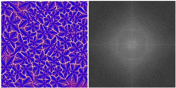
The phase field image shows the solidification structure calculated for an Mg-3Al alloy. The nuclei of the grains were located randomly with however the constraint that they should be at some minimum distance from the other nuclei. This leads to some regularity in the space distribution of the grains and should also affect solute distribution. This image has 2000x2000 points, 10x10 grains.

Figure 1 – Initial phase field image and its FFT transform

Characterization of the correlations in the images

That there is some correlation in the solute distribution may be crudely investigated by evaluating the average solute content along horizontal and vertical lines. The results have been plotted in figure 2. It is seen that there is an effect of the border of the calculation field, with higher average solute contents on about 10 lines all around the calculation box. Away of the boundary, the pseudo-regular oscillations of the average content are certainly related to the structuration of the microstructure.

2 3 4 5 6 7 8 0 500 1000 1500 2000 horizontal vertical C B Figure 2 -

This can be much more precisely studied by recording the variogram of the chemical map. The variogram is given as the square of the difference between two points distant by a vector h (the size of the vector will be given here in pixels) that is averaged over all the selected pairs of points. The variogram 2.γ(h) is thus a directional quantity that writes:

[[[[

]]]]

∑

∑

∑

∑

According to this equation, the variogram increases from 0 when h=0 to a value that is the variance for a random distribution when h is large enough for the pairs of points (x; x+h) to be non-correlated. In between, the variogram may present oscillations that are illustrative of space correlation between values at points x and x+h. As a matter of fact, it is generally useful to average such local variograms, this is called regularization. In an attempt to do so, the variogram was calculated over three series of 100 lines selected in the middle of the image. It is seen in figure 3 that all three variograms show two types of oscillations, small ones with a periodicity of about 10 pixels and larger ones with a periodicity in between 200 and 300 pixels. 0 2 4 6 8 10 12 14 0 200 400 600 800 1000 950-1050 1000-1100 1100-1200 C B Figure 3 -

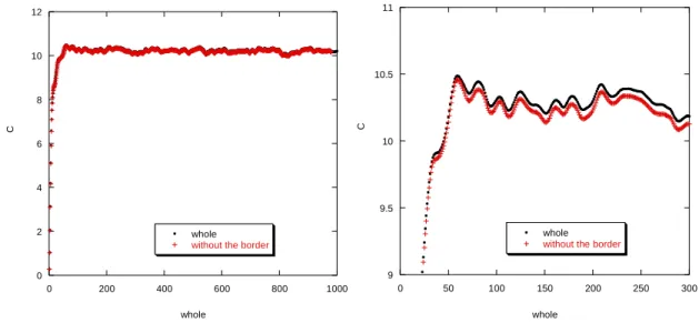
Going further, the variogram was calculated on the whole image and on the image without the border. Figure 4-a shows the two curves thus obtained, figure 4-b an enlargement for h lower than 300 pixels. It is seen that they are hardly differentiated on figure 4-a because they show the same behaviour with only a slight shift as illustrated in figure 4-b. On both graphs, the curves appear still noisy even after regularization, though the oscillations have been smoothed by averaging. The smallest oscillations present a wavelength of about 10 pixels that is still very well marked (figure 4-b), while the largest ones are less well defined with wavelength in the range 150 to 200 pixels. The former may be associated to secondary dendrite arm

spacings, the latter to the average grain size (200 pixels).

0 2 4 6 8 10 12 0 200 400 600 800 1000 whole

without the border

C whole 9 9.5 10 10.5 11 0 50 100 150 200 250 300 whole

without the border

C

whole

Figure 4 – a and b

Resampling

Resampling was performed by implementing grids of N=10x10 points with a first point selected at random. The grid size was the same in x and y directions, set first at 40 points, i.e. higher than the DAS value seen in figure 1 but much smaller than the average grain size at 200 pixels. Owing to the length of the grid, the location of the first point was selected in the range 1 to 1600 pixels for x and for y. For other grid steps, this latter range was modified accordingly.

Once obtained the 100 composition values, they were sorted in increasing order. Figure 5 shows three different cumulative distributions where it is seen that the scatter of the data is low at low fN values, and then increases dramatically for finally decrease again when fN gets

closer to 100%. The increase has been already described [Yan00] and the very large scatter should be related to measurements close to the interface between primary phase and eutectic areas. I do not understand why the last portion of the curves, at high fN values, shows a slope

rather than being at constant solute content if it represents eutectic data. Janin, is that a numerical feature or due to solid state diffusion.

0 2 4 6 8 10 0 20 40 60 80 100 So lu te c o n te n t (w t. % ) f N Figure 5 -

A systematic study was then performed by recording 1000 distributions for various grid step sizes, between 10 and 180 pixels, with the first point randomly selected in the appropriate area of the image. The same record was also performed for a random implementation of all points. The standard deviation of the composition associated at selected values of fN, every 10 %

from fN=5 to fN=95 %, were used to investigate the quality of the sampling procedure. In

addition, the standard deviation of the average solute content as estimated from the whole distribution curves was also evaluated.

The results are shown in the figure 6, where the data at abscissa 0 relate to the average composition. It is seen that the standard deviation on the average solute content is highest for the smallest grid step at 10 pixels, as expected. It then decreases and stabilizes at 0.38 for all other grid steps, but appears higher than the value for random sampling which is 0.23. This

difference is certainly du to the microstructure, it corresponds to an additional variance that amounts to {(0.38)2-(0.23)2}=0.09. 0 0.5 1 1.5 2 0 20 40 60 80 100 au hasard pas 10 pas 20 pas 40 pas 80 Pas 160 S ta n d a rd e rr o r f_N Conclusion

As previously concluded by Yang et al. [Yan00], 100 grid measurements may be quite sufficient to evaluate the shape of the distribution curves at low fN values. Care should be

taken to have a grid step large enough with respect to the microstrucre features, in particular larger that the secondary dendrite arm spacing as stressed by Gungor [Gun89]. This perquisite does not however ensure that the evaluation of the average solute content is optimized, and it has been shown that using regular grid introduces a systematic additional variance when compared to random sampling.