Analyse fréquentielle complète des crues dans le bassin Abiod Biskra (Algérie) = Complete Flood Frequency Analysis in Abiod Watershed Biskra (Algeria).

ANALYSE FREQUENTIELLE COMPLETE DES CRUES DANS LE BASSIN ABIOD, BISKRA (ALGERIE) COMPLETE FLOOD FREQUENCY ANALYSIS IN ABIOD

WATERSHED, BISKRA (ALGERIA)

Analyse fréquentielle complète des crues dans le bassin Abiod Biskra (Algérie)

Complete Flood Frequency Analysis in Abiod Watershed

Biskra (Algeria)

Sana BENAMEUR1, Abdelkader BENKHALED*2, Djamel MERAGHNI1, Fateh CHEBANA3, & Abdelhakim NECIR1

1_{Laboratory of Applied Mathematics, University of Biskra, Po Box 145, RP 07000 Biskra, Algeria}

2

Research Laboratory in Subterranean and Surface Hydraulics -LARHYSS, University of Biskra, Po Box 145, RP 07000 Biskra, Algeria

3_{INRS-ETE, University of Quebec, 490 rue de la Couronne, Québec, QC, Canada}

*

Corresponding author: fateh.chebana@ete.inrs.ca

Rapport INRS R1607

© INRS, Centre - Eau Terre Environnement, 2015 Dépôt légal, Bibliothèque nationale du Québec Dépôt légal, Bibliothèque et archives Canada

ABSTRACT Extreme hydrological events, such as floods and droughts, are one of the natural

disasters that occur in several parts of the world. They are regarded as being the most costly natural risks in terms of the disastrous consequences in human lives and in property damages. The main objective of the present study is to estimate flood events of Abiod wadi at given return periods at the gauge station of M’chouneche, located closely to the city of Biskra in a semi-arid region of Southern-East of Algeria. This single gauge station drains an important area. The motivation of the station and area choices is due to the existence of a dam to the downstream. This is a problematic issue in several ways including the field of the sedimentation and the water leaks through the dam during floods. A complete frequency analysis is performed on a series of observed daily average discharges, including classical statistical tools as well as recent techniques. The obtained results show that the Peaks-Over-Threshold approach based on the Generalized Pareto distribution (GPD) is more appropriate in this case. This study also indicates the importance of the continuous data monitoring at this station.

Key words : Frequency analysis ; Peaks-Over-threshold ; Generalized Pareto distribution ;

1. Introduction

The study of floods is a subject which arouses more and more interest in the field of water sciences. In spite of their low rainfall, the basins of the arid and semi-arid areas represent a hydroclimatic context where the overland flows phenomena are significant and feed a network of very active wadis. The activity of these wadis is far from being negligible from the flood in terms of their frequency and intensity. One observes on these rivers exceptional flows which sometimes, surprise by their magnitude [18]. The Abiod wadi, in the area of Biskra, is a very representative river of these basins. Moreover, the existence of Foum El Gherza dam to the downstream for the irrigation of the palm plantations makes the area more sensitive with regard to the floods. The flood events of the years 1963, 1966, 1971, 1976 and 1989 remain engraved in the memory of the inhabitants. The flood event of 11- 12th September 2009 was one of the historic floods in the Zibans area [7]. It rains 80 mm in 24 hours, while the annual total of Biskra city reaches 100 mm. The damage were 9790 palm trees, 164 flooded houses, 744 destroyed greenhouses, 200 hectares of lost cultures. The last flooding at the time of this drafting paper is that produced in October 29th 2011. All the populations living downstream of the Foum El Gherza dam were evacuated. The floods mainly occur in September and October and especially originate from exceptional storm events.

Describing and studying these situations could help in preventing or at least reducing severe human and material losses. The strategy of prevention of flood risk should be founded on various actions such as risk quantification. On this aspect, various methodological approaches can contribute to this strategy, among which flood Frequency Analysis (FA). Frequency analysis of extreme hydrological events, such as floods and droughts, is one of the privileged tools by hydrologists for the estimation of such extreme events and their return periods. The main

objective of FA approach is the estimation of the probability of exceedance P X





accomplished by fitting a probability distribution F to large observations in a data set. Two approaches were developed in the context of extreme value theory (EVT). The first one, usually based on the generalized extreme value distribution (GEV), describes the limiting distribution of a suitably normalized annual maximum (AM) and the second uses the generalized Pareto distribution (GPD) to approximate the distribution of Peaks-Over-Threshold (POT). For more details regarding this theory and its applications, the reader is referred to the textbooks of Embrechtes et al. [23],Reiss and Thomas [54] and Beirlant et al. [6].

Many FA models should be tested to determine the best fit probability distribution that describes the hydrologic data at hand. Specific distributions are recommended in some countries, such as the Log-normal (LN) distribution in China [10]. In the United States, the Log-Pearson type 3 distribution (LP3) has been, since 1967 [NRC, 47], the official model to which data from all catchments are fitted for planning and insurance purposes. By contrast, the United Kingdom endorsed the GEV distribution [NERC, 48, 49] up until 1999. The official distribution in this country is now the generalized logistic (GL), as for precipitation in the United States [61]. There are several examples where a number of alternative models have been evaluated for a particular country, for example Kenya [46], Bangladesh [35], Turkey [5] and Australia [60]. Nine distributions were used with data from 45 unregulated streams in Turkey by Haktanir [26] who concluded that two parameter Log-normal (LN2) and Gumbel distributions were superior to other distributions. Recent research was conducted by Ellouze and Abida [22] in ten regions of Tunisia. They found that the GEV and GL models provided better estimates of floods than any of the

reveals that the POT procedure is more advantageous than the AM in the case of short records. Lang et al. [41] develop a set of comprehensive practice-oriented guidelines for the use of the POT approach. Tanaka and Takara [57] has examined several indices to investigate how to determine the number of upper extremes rainfall best for the POT approach.

In the Algerian hydrological context, during the last two decades many authors have used several approaches to study the associated risks. Recently, Hebal and Remini [28] studied flood data from 53 gauge stations in northern Algeria, between 1966 and 2008. They found that 50 %, 25 % and 22 % of the samples follow respectively the Gamma, Weibull and Halphen A distributions. Bouanani [12] performed a regional flood FA in the Tafna catchments and concluded that the AM flows fit better to asymmetric distributions such as LP3, Pearson 3 and Gamma. The FA was also used in the sediment context by Benkhaled et al. [8] where the LN2 distribution was selected in the case of the same station considered in the present study, i.e. M’chouneche gauge station on Abiod wadi.

To the best knowledge of the authors, apart from Benkhaled et al. [8], the flood FA approach has not yet been performed on data collected at this station. The primary aim of this paper is to perform a FA to the Abiod wadi flow data. Specifically, the objective of this analysis is to choose the appropriate approach among AM and POT. In methodological terms, all the steps constituting FA are performed from data examination to risk assessment including hypotheses testing and model selection. Due to the high importance of the latter and its impacts, more recent techniques are employed to select the appropriate distribution that fit better to the tail. A relatively large number of known distributions fit well the center of the data whereas the focus in FA is on the distribution tail. To this end, tail classification and specific graphical tools are employed, see El Adlouni et al. [21] for more technical details.

The paper is organized as follows. In Section 2, the study area and the data set are briefly described. Section 3 is devoted to the FA methodology. The results of the study are presented and discussed in Section 4. Concluding remarks are reported in Section 5.

2. Study area and data

In this section, we present the region where the site of interest is located, followed by a description of the available data.

2.1 Study Area

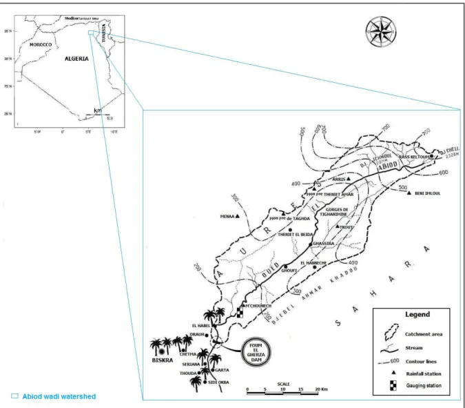
The Abiod wadi watershed, with an area of 1300 Km2, is located in the Aurès massif in the southern east of Algeria in North Africa (Figure 1). It is part of the endorheic watershed Chott Melghir. The wadi length is 85 km from its origin in the Chelia (2326 m high) and Ichemoul (2100 m high) mountains. After crossing Tighanimine, the wadi gradually flows into the canyons of Ghoufi and M’chouneche gorges, and then opens a path to the plain until the Saharian gorge Foum el Gherza. The valley of the wadi is mainly composed of sedimentary rocks, comprising alternating limestone, marl, soft sediments (sandstones, conglomerates) and some evaporates (gypsum) dated of Paleogene.

The watershed is characterized by its asymmetry, a mountainous area in the north to over 2000 m (Chelia) and another low area in the south (El Habel 295 m). The relief is rugged with slopes ranging between 12.5% and 25% for half of the area, and from 3% to 12.5% for another 40% of the area. Land cover is a mix of rocky outcrops, highly eroded soil, sparse vegetation, a few forests, crops, gardens and pastures [27]. In the orographic and hydrographic points of view, Abiod wadi is characterized by two distinct climatic regions: the Aurès, where rainfall averages

450 mm/year, and the Sahara plain with mean rainfall 100-150 mm/year. The climate of Abiod wadi watershed is thus semi-arid to arid. Along Abiod wadi to the Foum El Gherza dam there are six rainfall stations, and one hydrometric station located 18 km upstream of the dam, as shown in Figure 1.

2.2 Data Description

The data set used in this study is provided by the National Agency of Hydraulics Resources

(ANRH) of Biskra. It consists of the daily average discharges Q1, ,QN _(with N8034_),

collected at the gauge station of M’chouneche over 22 years from 1972 to 1994. The entire time series is represented in Figure 2. In addition, this figure shows the daily flow for each hydrological year (i.e. from September 1st to August 31th).

Note that the IACWD Bulletin 17B [1] suggests that at least 10 years of record are necessary to warrant a statistical analysis. For instance, Tramblay et al. [59] used a minimum of 10 years of daily data. The short data size can affect the choice of distributions, the quantile estimations, particularly those corresponding to large return periods and the extent of confidence intervals. The size of the used data in the present study is relatively large, to perform a FA, as in a number of similar studies [15].

In order to select the extreme data series used in FA, two approaches are considered: AM and POT, usually associated to GEV and GPD approximations respectively [30, 43]. Therefore, the estimation of flood magnitudes can be achieved by making use of two types of flood peak series, to be detailed in the next section.

3. Methodology

In this section, after defining the types of series, we briefly present the required elements to perform a hydrological FA. The latter is a statistical approach of prediction commonly used in hydrology to relate the magnitude of extreme events to a probability of their occurrence [16]. It allows, for the selected station, to estimate the flood quantiles of given return periods. In general, FA involves four main steps:

(i) characterization of the data and determination of the usual statistical indicators, such as the mean, the standard-deviation, the coefficients of skewness (Cs), kurtosis (Ck) and variation (Cv) and detection of outliers,

(ii) checking the basic hypotheses of FA, i.e. homogeneity, stationarity and independence, applicability on the studied data set,

(iii) fitting of probability distributions, estimation of the associated parameters and selection of the best model to represent the data, and

(iv) risk assessment based on quantiles or return periods, [e.g. 11, 14, 26, 52].

3.1. Annual Maximum Series

In the AM series framework, the daily flow series for each jth hydrological year, is replaced by its largest flood denoted Mj (see Figure 3) for the data of the present study. The extracted series

1, , n

M M _{(n is the number of years, heren22), is a random sample from some underlying}

EVT. Indeed, the AM series can be modeled by one of the extreme value distributions referred to as GEV distributions and briefly described in the following.

Let X_1,r X_2,r   X_{r r,} be the order statistics pertaining to a sample X₁, ,X from a non-_r

negative random variable X with cumulative distribution function (cdf) F. The GEV approach is based on the well-known result by Fisher and Tippett [24]. This result show that the limiting distribution of the (suitably normalized) maximum X_{r r,} is a non-degenerate cdf defined for 𝑥 ∈ 𝑅 such that 1x0, by

 













where  is a real parameter, called extreme value index (EVI) or tail index, which governs the thickness of the distribution tail. Depending on the sign of this crucial index, X belongs to the class of Gumbel (Type I) if it is null, the class of Fréchet (Type II) if it is positive and to the class of Weibull (Type III) if it is negative. The first two models are the mostly used in real life applications. They include such distributions as exponential, Pareto, Burr, GPD, GEV, t-Student,

-stable ( 0  2) and log-gamma known to be appropriate for fitting heavy-tailed data very often encountered in fields like hydrology, meteorology, insurance and finance.

In the present paper, X represents the daily average discharge ( Q ) of the jth year ( j=1, ,22 ), r

the number of days of the same year andX_{r r,}  M_j .

All AM flows obtained from the extraction process are thus considered as reasonable maxima. In

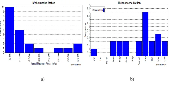
with very high amplitude are rare but not negligible which is consistent with their extreme aspects and also shows the importance of their study. More description is given in the result section. As seen in Figure 3, the culmination of September is very obvious because of the

frequency of hydro meteorological events, which represent approximately 27% ( 6 / 22 observations) of all data, as shown in Figure 4b. This would reflect the influence of the local climate.

3.2. Peaks Over Threshold Series

The data to be extracted and then used in this approach consist in the observations that exceed a

selected relatively high thresholdu . LetN denote the number of daily discharges exceeding u . _u

Then, the sample of excesses is defined as





j j

j i i u

E Q u s t Q u j N

In this approach the selection of an appropriate threshold is crucial. This approach is useful and has some advantages compared to the AM one, even though the latter is widely used. It is of particular interest in situations where the AM could not perform well especially in situation with little extreme data or the extracted extremes by AM cannot be considered as extremes in a physical or hydrological meaning.

3.2.1. GPD Approximation

Statistically, the distribution of the POT series ₁, ,

u

N

E E , can be determined by making use of

 

where 𝛾 ∈ 𝑅 _and  0 _{are respectively shape and scale parameters [31].}

Let F x_u

 





have the following result:

 

 

where q_F is the right end point of the cdf F. This result, due to Balkema and de Haan [4] and

Pickands [51], is one of the most useful concepts in statistical methods for extremes. It says that

for large threshold u , the excess cdf F is likeley to be well approximated by a GPD. _u

3.2.2. Threshold Selection

In order to obtain the asymptotic result in (3), the threshold u should be large enough which has as a consequence a satisfactory GPD approximation. The choice of the threshold is a crucial issue in the POT procedure. Indeed, selecting a threshold that is too low results in a large bias in the estimation, whereas taking one that is too high yields a big variance [23, section 6.4 and 6.5]. Hence, a compromise between bias and variance is to be found. To this end, one can minimize the asymptotic mean squared error, which is composed by the bias and variance. Furthermore, several graphical procedures are available to select u , such as the mean residual life (MRL), threshold choice (TC) and dispersion index (DI) plots. On the other hand, the choice of u can be

based on physical considerations, e.g. by identifying the flood level of the river of interest. For a

survey of the main selection procedures, see e.g. the paper of Lang et al [41].

3.3. Exploratory Data Analysis

The first step allows to check the data quality and to screen the data to avoid outlier effects. It also permits to obtain prior information, e.g. the shape, regarding the distribution to be selected. The presence of outliers in the data can have an important effect and causes difficulties when fitting a distribution [3] especially on the distribution upper part. The Grubbs and Beck [25] statistical test, based on the assumption of normality data, is designed to detect low and high outliers. In the case where the original data are not normal, they should be appropriately transformed. According to Section 1.8.3 in [52], this test is based on the following quantities:









where xand s are respectively the mean and standard deviation of the natural logarithms of the

sample, and k is the Grubbs-Beck statistic tabulated for various sample sizes and significance _n

levels by Grubbs and Beck [25]. For instance, at the 10% significance level, the following approximation is used 1/4 1/2 3/4 .62201 6.28446 – 2.49835 0.491436 – 0.037911 , 3 n n n n k     n (6)

The observations greater than x are considered to be high outliers, while those less than _H x are _L

taken as low outliers.

3.4. Testing Independence, Stationarity and Homogeneity

Three basic assumptions are required to correctly apply FA of extreme hydrological events, namely independence, stationarity and homogeneity of the data [11]. To verify these assumptions, three tests are widely used in the literature. The Wald-Wolfowitz test is employed for the independence, the homogeneity test of Wilcoxon is applied to check whether the data come from the same distribution or not and the Mann-Kendall test allows to verify stationarity of the data, i.e. the series does not present a trend over time. These three tests have the advantage of being non-parametric and are widely used in hydrological FA. In other words, they do not require any prior knowledge on the distribution of the data.

3.5. Parameter Estimation and Model Selection

The choice of the appropriate model is one of the most important issues in FA. In practice the distribution of hydroclimatic series is not known. Using the fitted probability distribution, it is possible to predict the probability of exceedance for a specified magnitude, i.e. quantile, or the magnitude associated with a specific exceedance probability. To estimate the parameters associated to the appropriate probability distribution from the data, popular techniques of parameter estimation are used in hydrology, including the methods of Maximum Likelihood (ML) [e.g. NERC, 17, 49], Moments (MM) and Probability Weighted Moments (PWM) [e.g. 13, 32]. The latter is equivalent the L-moment method which is widely used in hydrological FA [29]. Several studies are presented by focusing on the parameter estimation of a specific distribution to

indicate the appropriate method, such as the EVI using the generalized ML method [44]. Chebana

et al [13] estimated the Halphen distribution parameters using a mixed method.

The choice of the adequate distribution is determined on the basis of numerous classical and recent statistical tools, including graphical representations and goodness-of-fit tests. Due to the importance of the distribution impact in FA, these tools should be exploited. This point is widely studied in the literature [8, 19, 21, 28, 31, 39, e.g. 50].

In the literature, it is well-known that graphical display is essential whenever the user is confidante that a derived flood frequency model is consistent with the data [IH, 34, NERC, 49]. The problem with this approach lies in its subjective character owing to the fact that it is based only on the judgment of the hydrologist. Therefore, complement non-graphical tools should be considered.

Several standard statistical goodness-of-fit tests are reported in the literature for data modeling. We can cite the general tests of Pearson (Chi-squared, Chi2), Kolmogorov-Smirnov (KS), Cramer-von Mises and the normality specific Shapiro-Wilk (SW) test. Nonetheless, these decision procedures are not perfectly suited for extreme value distributions, because they are not sensitive enough to deviations in the distribution tails. Several transformations have been proposed to overcome the limitations of the aforementioned tests [36, 40, 42]. Since we focus on the tail of the distribution, the Anderson-Darling test is more appropriate (Ahmad et al., 1988).

The probability distributions that are appropriate for hydrology data are those with heavy tails. A number of them are listed for instance in [37, 52, 55]. In order to select the appropriate distribution among those which passed the goodness-of-fit tests, one or more criteria are required.

To this end, one can consider the Akaike and Bayesian information criterion (AIC, BIC) respectively proposed by Akaike [2] and Schwartz [56]. They are given by:

2ln 2 ,

AIC  L k (7)

2ln 2 ln

BIC  L k m (8)

where L is the likelihood function, the number of parameters and m the sample size.

The best fit is the one associated with the smallest criterion AIC or BIC values [19, 28, 52].

3.6. Quantile Estimation

Once the appropriate distribution selected, the quantiles and return periods can be evaluated. The quantile estimation for various recurrence intervals is the main goal in hydrological practice. The notion of return period for hydrological extreme events is commonly used in FA, where the objective is to obtain reliable estimates of the quantiles corresponding to given return periods of scientific relevance or government standard requirements [52]. In the FA context the uncertainty decreases with the sample size whereas it increases with the return period when estimating quantiles. The uncertainty can be seen as the unexplained variance [38].

In many environmental applications the sample size is rarely sufficient to enable good extreme quantiles estimations. Usually, a quantile of return period T can be reliably estimated from a data record of length n if T<n. However, in many cases, this condition is rarely satisfied –since typically n<50 for hydrological applications based on annual data [31].

4. Results and discussion The application of the presented methodology in section 3 to the data

described in section 2 leads to the following results, obtained by the means of the packages stats, evir and POT of the statistical software R [33] and also by using the HYFRAN-PLUS software [20].

4.1. Exploratory Analysis and Outlier Detection

From Figure 5, it appears that the whole daily data series vary from a minimum value of 0m3/s

corresponding to many dry days, to a maximum value of 78.57m3/s recorded on September 21st,

1989. The average flow of 0.39m3/s is a relatively low in comparison with other tributary wadis

of Chott Melghir like El Hai wadi and Djamorrah wadi [45]. The standard-deviation of

3

2.48m /s yields a coefficient of variation equal to 6.39. The box-plot in Figure 6 Figure 6

clearly shows the existence of extreme values. Indeed, the median (0.10m3/s ) is close to both

25th and 75th percentiles (0.04m3/s and0.20m3/s ). In addition to this graphical consideration,

the values of skewness and kurtosis (20.51m3/s and 498.59m3/s respectively) eliminate the

Gaussian model. In particular the very large value of the kurtosis indicates longer and fatter distribution tails, urging us to focus on heavy-tailed models

From Figure 2 we observe that the AM approach is not relevant for the Abiod wadi data. Indeed, for some years even the highest discharges are very low and probably are not extreme events (for example 1973-1975, 1978-1979, 1984-1985, ...). On the other hand, for some years several high discharges are observed like in 1972-1973, 1976-1977, but only one is selected by the AM sampling at each of those years. This suggests that the POT approach would be more appropriate, and would lead to a more homogeneous sample of extreme discharges. This method starts with

the selection of a convenient threshold, then the consideration of the observations that exceed this threshold.

4.1.1. Threshold Selection

In this study, we adopt one of the available graphical tools, namely the TC-plot. From Figure 7

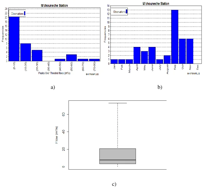
we can choose a threshold valueu5.6m3/s, which results in an excess series of size 58. However, as recommended by many authors [9, 41, 58], this data set must be reduced in order to avoid the effects of dependence. We eliminated the peaks being obviously part of the same flood, and in order to keep the character of flood seasonality, we retain three peaks per year over the recorded period. Thus, the length of the data series becomes 42 . Figure 8 shows the distribution of these excesses and Table 1 summarizes their elementary statistics.

The positive skewness coefficient Cs=1.62 reveals that the data is right skewed relative to the mean excess, as shown in Figure 8a.

In Figure 8a, the data Ej are arranged by classes, of length 10 m3/s each, with the associated frequencies. It can be seen that some values are more frequent than others and that the majority of excesses have a low value varying between 0 and 10 m3/s. Figure 8b, where the data are arranged according to the months of appearance, shows that the peaks generally occur in the fall season.

In order to detect outliers, the quantities x and _H x are found to 508.31 and 0.08 respectively. _L

Since there is no value greater than x and nor less than_H x , we conclude that, at the significant _L

4.2. Testing the Basic FA Assumptions

The results of the required hypothesis testing on the considered data are given in Table 2. Applying Wilcoxon, Kendall and Walf-Wolfowitz tests respectively, we conclude that the homogeneity, stationarity and independence of the excesses are accepted at any of standard significance levels (1%, 5% and 10%). Note that for the homogeneity test, we split the data in two sub-series 1972-1981 and 1982-1994 (any other subdivision led to the same conclusion. The homogeneity can also be noted in Figure 8a where there is only one mode (the highest frequency).

4.3. Model Fitting

To fit a statistical distribution, we consider three commonly used estimation methods of the GPD parameters (ML, MM, and PWM). Then we perform the Anderson-Darling test to check the goodness-of-fit of the model. The results are summarized in Table 3. In view of the large P-values, we deduce that the GPD can be accepted as an appropriate model for the excess at any standard significance level (for instance 5%).

To discriminate between the obtained models, we use the AIC and BIC criteria. The last two columns of Table 3 as well as Figure 9b favor the GPD of the ML fitting method. We illustrate the goodness of fit of the excesses to this model in Figure 9a. Furthermore, this ML-based will be used for quantile estimation in the following section.

Note that the ML and PWM results are very similar whereas those of the MM results are slightly different but remain in the same range.

4.4. Quantile Estimation

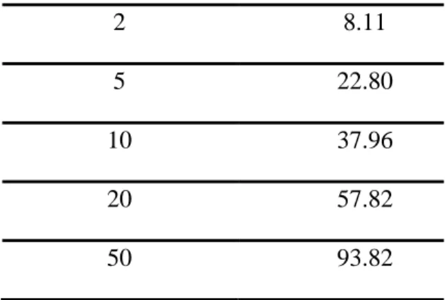
The estimation of extreme quantiles for different return periods should take into consideration the record period and the right tail of the distribution. The formally gauged record represents a relatively small sample of a much larger population of flood events. Thus, the extrapolation for long return periods is less accurate. In the M’chouneche station only the following return periods were considered for the estimation of quantiles: 2, 5, 10, 20 and 50 years as presented in Table 4. From this result, the highest flood observed in the 1972-1994 period would correspond to an event with a 30-year recurrence interval.

The confidence interval is a way to show the uncertainty. It is based on the distribution of the quantity of interest (papameter, quantile, etc). For the GPD, the confidence intervals associated to the estimation of parameters and quantiles are obtained through asymptotic results (Hosking and Wallis, 1987). For the present case-study, this can be seen from Figure 9c.

5. Conclusions

The study of the Algerian wadis floods remains a quasi-unknown field as only some very specific indications are given in the Algerian hydrological directories. Floods are one of the basic features of a stream regime. The present study, which is the first one carried out in southern east of Algeria, in the context of FA. Mean daily discharges data recorded at the gauging station of M’chouneche in Abiod wadi, near Biskra, are available and considered in the present study. Due

to the high inter-annual variability of the data as well as to the relatively short record length, the AM approach is not adapted to this analysis. Hence, in this paper, we considered a more appropriate procedure, namely the POT method.

The purpose of this work is to provide a suitable model for the excesses over a chosen threshold. This allows to estimate extreme flood events of given return periods. A complete FA was applied including appropriate tools, commonly used in hydrology.

The issue of threshold selection was dealt by the means of a graphical tool. Several fitting methods have led to different GPD models and according to the results, the ML-based distribution was adopted.

Because of the short record length, only return periods of 2, 5, 10, 20 and 50 years were considered. It was found that most of extracted data corresponded to frequent events. The return period of the largest recorded flood is about 30 years.

As a conclusion, we should emphasis that, in addition to the quality of data and sample size, the right choice of a GPD model heavily depends on the threshold. To improve the flood FA at this site, future studies should focus on the importance of data monitoring. However, this conclusion even it is not new in FA, it is important for the studied area where this is the first time to be studied. It emphasis and confirms the importance of this issue, especially for local government and decision makers.

Acknowledgments

The authors express their gratefulness to the financial support of Canada's International Development Research Centre (IDRC). The data used in this study where provided by the National Agency of Water Resource of Algeria (ANRH).

References

[1] (IACWD), I. C. o. W. D. Guidelines for determining flood flow frequency: Bulletin 17B (revised and corrected). Hydrol. Subcomm., Washington, D.C, 281982).

[2] Akaike, H. A new look at the statistical model identification. Automatic Conrol, IEEE, 19, 6 (Dec 1974), 716 - 723.

[3] Ashkar, F. and Ouarda, T. B. M. J. Robust estimators in hydrologic frequency analysis. In: Engineering Hydrology (edited by C.Y Kuo) Am. Soc. Civ. Eng. New York, USA1993), 347-352. [4] Balkema, A. A. and de Haan, L. Residual Lifetime at Great Age. Annals of Probability, 21974), 792-804.

[5] Bayazıt, M., Shaban, F. and Onoz, B. Generalized Extreme Value Distribution for Flood Discharges. Turkish Journal of Engineering and Environmental Sciences, 21, 2 1997), 69-73. [6] Beirlant, J., Goegebeur, Y., Segers, J., Teugels, J., de Waal, D. and Ferro, C. Statistics of

Extremes: Theory and Applications. Wiley, 2004.

[7] Benazzouz, M. T. Flash floods in Algeria: impact and management. G-WADI meeting. Flash Flood Risk Management Expert Group. Meeting Cairo 25-27 September 2010, Egypt2010). [8] Benkhaled, A., Higgins, H., Chebana, F. and Necir, A. Frequency analysis of annual maximum suspended sediment concentrations in Abiod wadi, Biskra (Algeria). Hydrological

Processes2013).

[9] Beran, M. A. and Nozdryn-Plotnicki, M. J. Estimation of low return period floods.

Hydrological Sciences Bulletin, 22, 2 (1977/06/01 1977), 275-282.

[10] Bobée, B. Extreme flood events valuation using frequency analysis. A critical review.

Houille Blanche, 54, 7-8 1999), 100-105.

[11] Bobée, B. and Ashkar, F. The gamma family and derived distributions applied in hydrology. Water Resources Publications, 1991.

[12] Bouanani, A. Hydrologie, Transport solide et Modélisation. Etude de quelques sous bassins

de la Tafna. Université de Tlemcen, 2005.

[13] Chebana, F., Adlouni, S. and Bobée, B. Mixed estimation methods for Halphen distributions with applications in extreme hydrologic events. Stochastic Environmental Research and Risk

Assessment, 24, 3 2010), 359-376.

[14] Chebana, F. and Ouarda, T. B. M. J. Multivariate quantiles in hydrological frequency analysis. Environmetrics, 22, 1 2011), 63-78.

[15] Chebana, F., Ouarda, T. B. M. J., Bruneau, P., Barbet, M., El Adlouni, S. and Latraverse, M. Multivariate homogeneity testing in a northern case study in the province of Quebec Canada.

[16] Chow, V. T., Maidment, D. R. and Mays, L. W. Applied Hydrology. McGraw-Hill, New

York, NY1988).

[17] Clarke, R. T. Fitting distributions. Chapter 4 Statistical modeling in hydrology. Wiley1994), 39-85.

[18] Dubief, J. Essai sur l’hydrologie superficielle au Sahara. GGA, Direction du Service de la

Colonisation et de l’Hydraulique, Service des Etudes Scientifiques, Alger, 4571953).

[19] Ehsanzadeh, E., El Adlouni, S. and Bobee, B. Frequency Analysis Incorporating a Decision Support System for Hydroclimatic Variables. Journal of Hydrologic Engineering, 15, 11 2010), 869-881.

[20] El Adlouni, S. and Bobée, B. Système d’aide à la decision pour l’estimation du risqué hydrologique. IASH Publ, 3402010).

[21] El Adlouni, S., Bobée, B. and Ouarda, T. B. M. J. On the tails of extreme event distributions in hydrology. Journal of Hydrology, 355, 1–4 2008), 16-33.

[22] Ellouze, M. and Abida, H. Regional Flood Frequency Analysis in Tunisia: Identification of Regional Distributions. Water resources management, 22, 8 2008), 943-957.

[23] Embrechts, P., Klüppelberg, C. and Mikosch, T. Modelling Extremal Events for Insurance

and Finance. Springer, 1997.

[24] Fisher, R. A. and Tippett, L. H. C. Limiting forms of the frequency distribution of the largest or smallest member of a sample. Mathematical Proceedings of the Cambridge Philosophical

Society, 24, 02 1928), 180-190.

[25] Grubbs, F. E. and Beck, G. Extension of sample sizes and percentage points for significance tests of outlying observations. Technometrics, 14(Nov 1972), 847-854.

[26] Haktanir, T. Comparison of various flood frequency distributions using annual flood peaks data of rivers in Anatolia. Journal of Hydrology, 136, 1–4 1992), 1-31.

[27] Hamel, A. Hydrogéologie des systèmes aquifères en pays montagneux à climat semi-aride.

Cas de la vallée d’Oued El Abiod (Aurès). Université, Mentouri : Constantine, 2009.

[28] Hebal, A. and Remini, B. Choix du modèle fréquentiel le plus adéquat à l’estimation des valeurs extrêmes de crues (cas du nord de L’Algérie). Canadian Journal of Civil Engineering, 38, 8 2011), 881-892.

[29] Hosking, J. R. M. L-moments: analysis and estimation of distributions using linear combinations of order statistics. Journal of the Royal Statistical Society, 521990), 105–124. [30] Hosking, J. R. M. and Wallis, J. R. Parameter and Quantile Estimation for the Generalized Pareto Distribution. Technometrics 291987), 339-349.

[31] Hosking, J. R. M. and Wallis, J. R. Regional frequency analysis; an approach based on L-moments. Cambridge University Press1997), 224.

[32] Hosking, J. R. M., Wallis, J. R. and Wood, E. F. Estimation of the generalized extreme value distribution by the method of probability-weighted moments. Technometrics : . 271985), 257-261.

[33] Ihaka, R. and Gentleman, R. R: A Language for Data Analysis and Graphics. Journal of

Computational and Graphical Statistics, 5, 3 (1996/09/01 1996), 299-314.

[34] Institute of Hydrology (IH). Flood Estimation Handbook. Wallingford, U.K, 1999.

[35] Karim, M. A. and Chowdhury, J. U. A comparison of four distributions used in flood frequency analysis in Bangladesh. Hydrological Sciences Journal, 40, 1 (1995/02/01 1995), 55-66.

[36] Khamis, H. J. The delta-corrected Kolmogorov-Smirnov test for the two-parameter Weibull distribution. Journal of Applied Statistics, 24, 3 (1997/06/01 1997), 301-318.

[37] Kite, G. W. Flood and Risk Analyses in Hydrology. Water Resources Publications, Littleton,

Colorado, USA, 1871988).

[38] Koutsoyiannis, D. Hurst-Kolmogorov Dynamics and Uncertainty1. JAWRA Journal of the

American Water Resources Association, 47, 3 2011), 481-495.

[39] Koutsoyiannis, D. On the appropriateness of the Gumbel distribution for odeling extreme rainfall. In: Brath, A., Montanari, A., Toth, E. (Eds.), Hydrological Risk: Recent Advances in

Peak River Flow Modelling, Prediction and Realtime Forecasting. Assessment of the Impacts of Land-use and Climate Changes. Editoriale Bios, Castrolibero, Bologna; 303–319.2003).

[40] Laio, F. Cramer-von Mises and Anderson-Darling goodness of fit tests for extreme value distribution with unknown parameters. Water Resour. Res, W09308, 402004).

[41] Lang, M., Ouarda, T. B. M. J. and Bobée, B. Towards operational guidelines for over-threshold modeling. Journal of Hydrology, 225, 3–4 1999), 103-117.

[42] Liao, M. and Shimokawa, T. A new goodness-of-fit test for type-I extreme-value and 2-parameter weibull distributions with estimated 2-parameters. Journal of Statistical Computation

and Simulation, 64, 1 (1999/08/01 1999), 23-48.

[43] Madsen, H., Rasmussen, P. F. and Rosbjerg, D. Comparison of annual maximum series and partial duration series methods for modeling extreme hydrologic events: 1. At-site modeling.

Water Resources Research, 33, 4 1997), 747-757.

[44] Martins, E. S. and Stedinger, J. R. Generalized maximum-likelihood generalized extreme-value quantile estimators for hydrologic data. Water Resour. Res, 36, 3 2000), 737-744.

[46] Mutua, F. M. The use of the Akaike Information Criterion in the identification of an optimum flood frequency model. Hydrological Sciences Journal, 39, 3 (1994/06/01 1994), 235-244.

[47] National Research Council (NRC) Estimating probabilities of extreme floods: methods and

recommended research. National Academy Press, 1988.

[48] Natural Environment Research Council (NERC) Flood Studies Report. Wallingford:

Institute of Hydrology, In five volumes1999).

[49] Natural Environment Research Council (NERC) Flood studies report. London, 11975). [50] Ouarda, T. B. M. J., Ashkar, F., Bensaid, E. and Hourani, I. Statistical distributions used in

hydrology. Transformations and asymptotic properties. University of Moncton, 1994.

[51] Pickands, J. Statistical inference using extreme order statistics. Annals of Statistics, 3, 1 1975), 119-131.

[52] Rao, A. R. and Hamed, K. H. Flood Frequency Analysis. City, 2000.

[53] Rasmussen, P. F., Ashkar, F., Rosbjerg, D. and Bobée, B. The POT method for flood estimation: a review. In: Hipel, K.W. (Ed.). Stochastic and Statistical Methods in Hydrology and Environmental ngineering, Extreme Values: Floods and Droughts, Kluwer Academic, Dordrecht.

Water Science and Technology Library, 11994), 15-26.

[54] Reiss, R. D. and Thomas, M. Statistical Analysis of Extreme Values: With Applications to

Insurance, Finance, Hydrology and Other Fields. Birkhauser Verlag GmbH, 2007.

[55] Salas, J. D. and Smith, R. Computer Programs of Distribution Functions in Hydrology.

Colorado State. University, Fort Collins, Colorado, USA1980).

[56] Schwartz, G. Estimating the dimension of a model. The Annals of Statistics., 61978 ), 461-464.

[57] Tanaka, S. and Takara, K. A study on threshold selection in POT analysis of extreme floods.

IAHS-AISH publication, 2712002).

[58] Todorovic, P. and Zelenhasic, E. A Stochastic Model for Flood Analysis. Water Resources

Research, 6, 6 1970), 1641-1648.

[59] Tramblay, Y., St-Hilaire, A. and Ouarda, T. B. M. J. Frequency analysis of maximum annual suspended sediment concentrations in North America. Hydrological Sciences Journal, 53, 1 (2008/02/01 2008), 236-252.

[60] Vogel, R. M., McMahon, T. A. and Chiew, F. H. S. Floodflow frequency model selection in Australia. Journal of Hydrology, 146, 0 1993), 421-449.

List Of Tables

Table 1. Statistics summary of excess data set... 27

Table 2. Stationarity, independence and homogeneity tests results. ... 27

Table 3. GPD parameter estimation, Anderson-Darling goodness-of- fit test and

information criterion results. ... 28

Table 4. Estimated quantiles of excess flows from the ML-based GPD. ... 28

List Of Figures

Figure 1. Presentation of the Abiod wadi watershed. ... 29

Figure 2. Time series plot of the daily average discharge at M’chouneche station covering the period 01/09/1972-31/08/1994 (8034 observations, every hydrological year). ... 30

Figure 3. Time series plot of the AM flows at M’chouneche station covering the period 01/09/1972-31/08/1994 (22 observations). ... 31

Figure 4. Histogram of the AM flows at M’chouneche station covering the period

01/09/1972-31/08/1994, observations selected by a) flow classes b) month. ... 32

Figure 5. Time series plot of the daily average discharge at M’chouneche station covering the period 01/09/1972-31/08/1994. ... 33

Figure 7. Graphical results of threshold selection applied for daily average discharge of Abiod wadi at M’chouneche station (tc-plot), vertical line corresponding to the threshold.34

Figure 8. Distribution of excess series Ej at M’chouneche station a) Histogram by flow classes b) Histogram by month c) boxplot. ... 35

Figure 9. Best fitted distributions of excess flows at M’chouneche station a) distributions b) qqplot of ML-based GPD c) Return level plot ... 36

Table 1. Statistics summary of excess data set. Size 42 Minimum 0.02 Qu1 3.36 Median 7.83 Average 15.72 Qu2 19.92 Sd 19.70 Maximum 72.97 Cs 1.62 Ck 4.48

Qu1 and Qu2: 25th and 75th percentiles respectively.

Table 2. Stationarity, independence and homogeneity tests results.

Tests Statistic Value P-value

Stationarity (Kendall) 0.48 0.63 Independence (Wald-Wolfowitz) 0.94 0.35

Table 3. GPD parameter estimation, Anderson-Darling goodness-of- fit test and information criterion results.

Method Scale Shape Statistic value P-value AIC BIC

ML 10.19 0.39 -0.55 0.49 315.68 326.63 MM 12.86 0.18 -0.83 0.58 316.61 327.56

PWM 10.10 0.36 -0.86 0.59 315.72 326.68

Table 4. Estimated quantiles of excess flows from the ML-based GPD.

Return period (years) Estimated quantile

2 8.11

5 22.80

10 37.96

20 57.82

Figure 2. Time series plot of the daily average discharge at M’chouneche station covering the period 01/09/1972-31/08/1994 (8034 observations, every hydrological year).

Figure 3. Time series plot of the AM flows at M’chouneche station covering the period 01/09/1972-31/08/1994 (22 observations).

a) b)

Figure 4. Histogram of the AM flows at M’chouneche station covering the period 01/09/1972-31/08/1994, observations selected by a) flow classes b) month.

Figure 6. Box plot of daily average discharge at M’chouneche station.

Figure 7. Graphical results of threshold selection applied for daily average discharge of Abiod wadi at M’chouneche station (tc-plot), vertical line corresponding to the threshold.

a) b)

c)

Figure 8. Distribution of excess series Ej at M’chouneche station a) Histogram by flow classes b) Histogram by month c) boxplot.

a)

b) c)

Figure 9. Best fitted distributions of excess flows at M’chouneche station a) distributions b) qqplot of ML-based GPD c) Return level plot