A Distributed Hydrological Modelling System to Support Hydroelectric Production in Northern Environments under Current and Changing Climate Conditions.

(1)

to Support Hydroelectric Production in Northern Environments

under Current and Changing Climate Conditions

Progress Report presented to : Yukon Energy Corporation

#2 Miles Canyon Road Box 5920

Whitehorse YT Y1A 6S7

Alain N. Rousseau, P.Eng., Ph.D. Stéphane Savary, Jr Eng. (EIT), M.Sc.

Sébastien Tremblay Laurie Caillouet Cheick Doumbia

Julien Augas

Centre Eau Terre Environnement

Institut national de la recherche scientifique (INRS-ETE) 490, rue de la Couronne, Québec (QC), G1K 9A9

Progress report R1768

(2)

(3)

Project team

Lead authors

Alain N. Rousseau Institut national de la recherche scientifique Eau Terre et Environnement Stéphane Savary Institut national de la recherche scientifique Eau Terre et Environnement Sébastien Tremblay Institut national de la recherche scientifique Eau Terre et Environnement Laurie Caillouet Institut national de la recherche scientifique Eau Terre et Environnement Julien Augas Institut national de la recherche scientifique Eau Terre et Environnement Cheick Doumbia Institut national de la recherche scientifique Eau Terre et Environnement Contributors

Jos Samuel Northern Climate ExChange, Yukon Research Centre, Yukon College Brian Horton Northern Climate ExChange, Yukon Research Centre, Yukon College Maciej Stetkiewicz Northern Climate ExChange, Yukon Research Centre, Yukon College Marc-André Lavigne Yukon Energy Corporation

Ron Gee Yukon Energy Corporation

Shannon Mallory Yukon Energy Corporation Goran Serckovic Yukon Energy Corporation Blaise Gauvin St-Denis Ouranos

Diane Chaumont Ouranos

Disclaimer

This report, including any associated maps, tables and figures (the “Information”) conveys general comments and observation only. The Information is provided by the Institut national de la recherche scientifique Centre Eau Terre Environnement (INRS-ETE) on an “AS IS” basis without any warranty or representation, express or implied, as to its accuracy or completeness. Any reliance you place upon the information contained here is your sole responsibility and strictly at your own risk. In no event will the INRS-ETE be liable for any loss or damage whatsoever, including without limitation, indirect or consequential loss or damage, arising from reliance upon the Information.

(4)

(5)

Acknowledgements

We gratefully acknowledge the financial support from the Natural Sciences and Engineering Research Council of Canada (NSERC) and Yukon Energy Corporation (YEC).

This project would also not have been possible without contributions from staff and students at the INRS-ETE namely: Pascal Castellazzi, Guillaume Talbot and Alexandre Alix.

The staff at YEC represents one of the driving forces behind this project, thus, we would like to acknowledge their strong contributions towards the achievement of the different project objectives (a.k.a., work packages).

(6)

(7)

List of Figures

Figure 2.1 DEMs and stream and lake networks: (a) Mayo Watershed (b) Aishihik Watershed and (c) Upper

Yukon River watershed. ... 15

Figure 2.2 Land cover maps: (a) Mayo, (b) Aishihik and (c) Upper Yukon River Watersheds. ... 20

Figure 2.3 Soil texture triangle (Moeys, 2009). ... 22

Figure 2.4 Soil type maps: of (a) Mayo, (b) Aishihik) and (c) Upper Yukon River Watersheds. ... 24

Figure 2.5 PHYSITEL – Input data and data processing. ... 25

Figure 2.6 Modelled hydrological networks for: (a) Mayo, (b) Aishihik and (c) Upper Yukon River Watersheds. . 28

Figure 2.7 RHHU / Hillslope delineation of Mayo (a) Aishihik (b) and (c) Upper Yukon River Watersheds. ... 29

Figure 2.8 Meteorological and hydrometric stations and snow survey sites for Mayo (a) Aishihik (b) and (c) Upper Yukon River Watersheds. ... 32

Figure 2.9 Mayo, Aishihik and Upper Yukon River Watersheds displayed using the HYDROTEL graphical user interface. ... 39

Figure 2.10 Example of workspace window of HYDROTEL. ... 39

Figure 2.11 Graphical comparisons of measured flows or calculated inflows with simulated flows or inflows for: (a) Sekulmun River, (b) Aishihik Lake, (c) Mayo Lake and (d) Yukon River (Whitehorse). ... 49

Figure 2.12 Graphical comparisons of measured flows or calculated inflows with simulated flows and inflows following data assimilation (DA) for: (a) Sekulmun River, (b) Aishihik Lake and (c) Mayo Lake. ... 52

Figure 2.13 Comparison of observed (Environment Canada) and reanalysed (CFSR, ERA-INT, JRA55, MERRA2 ) mean daily temperature and total annual precipitation at the scale of the Aishihik and Mayo. ... 56

Figure 2.14 Forecasting system flow chart (including working directory) for both NAEFS (a) and CanSIPS (b) meteorological forecasting ensembles. ... 59

Figure 2.15 Print screen of the hydrological forecast system GUI. ... 60

(10)

(11)

List of Tables

Table 2.1 Spatial data for watershed discretization using PHYSITEL ... 12

Table 2.2 Regrouped classes of the MODIS classification for the Mayo and Aishihik watersheds ... 17

Table 2.3 Regrouped classes of the CIRCA classification for the Mayo and Aishihik Watersheds ... 18

Table 2.4 Modelling characteristics of the discretized Mayo, Aishihik and Upper Yukon River Watersheds. ... 30

Table 2.5 Meteorological stations of the Mayo, Aishihik and Upper Yukon River Watersheds. ... 33

Table 2.6 Hydrometric stations of the Mayo, Aishihik and Upper Yukon River Watersheds. ... 36

Table 2.7 Snow survey sites for the Mayo, Aishihik and Upper Yukon River Watersheds. ... 37

Table 2.8 HYDROTEL sub-model and simulation Options ... 40

Table 2.9 Monthly values of slope and intercept of the linear regression equation to estimate the Aishihik River station (08AA010) flows when measurements at the Giltana Creek hydrometric station (08AA009) are missing. ... 44

Table 2.10 Calibration performance in corroborating with observed flows or reconstructed inflows for the 2010-2016 period for each watershed. ... 49

Table 2.11 Model performance in representing observed flows or inflows for the 2016 year. ... 52

(12)

(13)

Summary

The objective of this project is to implement a distributed hydrological modeling system on key watersheds of the Yukon Energy Corporation (YEC). This system will be used for hydrological forecasting (i.e., inflows and stream flows) with different lead times (e.g., 1-14 days) to assist hydroelectric operations as well as seasonal and long-term planning. Long-term planning will use the modeling system to predict impacts of climate change on inflows and flow availability, timing and extreme events. The results will provide strategic information for the assessment of potential energy projects to supply Yukon with enough electricity to meet projected demands. Understanding climate change and associated effects will be useful to other processes such as relicensing activities. This progress report provides a brief description of the state of the work packages (WPs) conducted over the course of the first year of this project study and highlights the tasks to be conducted over the next year.

(14)

(15)

List of acronyms

ARD Applied Research and Development

BC British Columbia

CanSIPS Canadian Seasonal and Inter-annual Prediction System CaPA Canadian Precipitation Analysis

CGCM Canadian General Circulation Model

CMIP5 Coupled Model Intercomparison Project Phase 5 CRD Collaborative Research and Development

DA Data Assimilation

DEM Digital Elevation Model

ECCC Environment and Climate Change Canada EnKF Ensemble Kalman Filter

ENSO El Niño Southern Oscillation ESP Ensemble Streamflow Prediction GDPS Global Deterministic Prediction System GEPS Global Ensemble Prediction System GIS Geographic Information System GUI Graphical user interface

HQP Highly Qualified Personnel

INRS Institut National de la Recherche Scientifique IPCC Intergovernmental Panel on Climate Change

MDDELCC Ministère du Développement Durable, de l’Environnement et de la Lutte aux Changements Climatique

NAEFS North American Ensemble Forecast System MSC Meteorological Service of Canada

(16)

NSERC Natural Sciences and Engineering Research Council of Canada PCIC Pacific Climate Impacts Consortium

PDO Pacific Decadal Oscillation

RCPs Representative Concentration Pathways RDPS Regional Deterministic Prediction System RHHU Relatively Homogenous Hydrologic Units RFS River Forecasting System

RSs River Segments

SWE Snow Water Equivalent SVD Singular Value Decomposition SVM Support Vector Machine

WP Work package

YC Yukon College

(17)

Context

In northern environments, limited hydro-meteorological networks and evolving climate conditions provide continuous challenges to water resource managers. YEC operates hydroelectric facilities under such conditions. For long-term resource planning exercises where capacity and predicted electrical load are analyzed to inform new projects, YEC does noes not currently factor in climate variability and change. Thus, there is a fundamental need to: (i) establish detailed knowledge of current and future hydro-meteorological conditions and (ii) assess the sensitivity of each hydroelectric facility to climate. To address these issues, YEC has recruited a multidisciplinary team of hydrology and climate change experts to jointly undertake an applied research project under NSERC Applied Research and Development (ARD) and Collaborative Research and Development (CRD) Programs. This research team includes members from the Northern Climate ExChange (NCE, part of the Yukon Research Centre at Yukon College), Institut national de la recherche scientifique (INRS, Quebec) and Ouranos (Consortium on regional climatology and adaptation to climate change, Quebec).

The team of experts is currently developing a hydrological modeling framework using existing data and providing context-specific studies and model advancements, tailored for northern environments, using a combination of field studies and cutting-edge data assimilation techniques. For NCE, the primary focus will be to develop an innovative data assimilation tool that YEC can use to perform accurate short-to-medium-term inflow and flow forecasting (daily and up to 1-year lead) and to optimize operational reservoir monitoring and management. Other tasks relate to providing support to the CRD project proposed by INRS (e.g., bias correction of weather forecast products; snow survey data). For INRS and with the collaboration of Yukon College, the focus will be on implementing a robust, distributed, hydrological modelling system for short-term (1-14 days) predictions (i.e., inflow and streamflow forecasting), seasonal projections (1-12 months) and long-term hydrological trends (30-year time periods, e.g., 2040-2070). NCE will use the forecasting framework provided by INRS to develop the aforementioned data assimilation tool. INRS will provide training to YEC professionals (operation of the inflow and streamflow forecasting system) and highly qualified personnel (HQP) to conduct research in northern hydrology and build the professional and technological capacities of YEC.

(18)

(19)

1. Introduction

Inflow and streamflow forecasts have proven to be of value for the operations of hydropower systems in Canada. Forecasts are often use with the dual purpose of maximizing energy production while providing flood control. For example, Hydro-Quebec and BC Hydro use forecasts to optimize hydropower system operations (Schaffer and Shawwash, 2014; Gignac et al., 2014; Martin et al., 2014) while Rio-Tinto Alcan operates hydroelectric plants to supply energy to aluminum smelters in Quebec and British-Columbia (Larouche et al., 2014). Both utility companies operate plants in northern environments where snowmelt represents a major hydrologic process. Meanwhile, the Quebec Ministry of Sustainable Development, Environment and Climate Change (MDDELCC) uses inflow forecasts to manage a considerable number of dams affected by significant spring freshets, several of them requiring real-time management (Turcotte and Lafleur, 2014). Uncertainty associated with the monitoring of snow water equivalent (SWE) and spatial distribution of snowpack adds complexity to forecasting the timing and volume of the spring freshet. YEC faces equivalent challenges in the operation of three hydroelectric dams, the Whitehorse, Aishihik and Mayo Facilities. The impacts of climate change on watershed hydrology, glacier dynamics and permafrost provide additional uncertainty when there is a need to asses long-term hydrological trends (30-year time periods, e.g., 2040-2070). YEC has recognised the need to account for climate change in the planning, management and relicensing (25-year license) of hydroelectric reservoirs. For YEC, there is also a need for basic short-term as well as mid-term seasonal forecasts. This latest requirement is in line with the need to support water resources mangers with environmental predictions with forecast ranges from 2 weeks to 12 months (National Academies of Sciences, Engineering and Medicine, 2016).

Hydrological forecasting requires the use of weather forecasts as inputs to a hydrological modelling system. Fort short-term forecasts, data assimilation techniques based on post-processing of model outputs or adjusting model inputs, state variables or parameters, are generally used to improve forecasts. For short lead times, weather forecasts are usually deterministic, while they are probabilistic (i.e., ensemble forecasts) for longer lead times (e.g., Thirel et al., 2008). Sene (2010) reports knowledge of correlations between large-scale atmosphere and oceanic structures (e.g., Pacific Decadal Oscillation, PDO, El Niño Southern Oscillation, ENSO) may be useful for long-term forecasts.

(20)

Furthermore, demand forecasts for energy supply along with reservoir/lake level constraints and/or downstream flow regulations, may then be used as inputs to an existing reservoir management model. The overarching goal of this project is to implement a distributed hydrological modelling system to support hydroelectric production in Yukon under current and changing climate conditions. Building from previous collaboration between NCE and YEC, the project increase the capacity for short and mid-term inflow forecast for the Mayo, Aishihik and Withehorse Facilites and assess potential change in flow volume and extreme events due to climate change in terms of severity, timing and frequency more specifically for Mayo and Aishihik Facilities. To achieve these goals, model advancements, tailored for northern environments, will require development or adaptation of permafrost, multi-layer snow and glacier modules, using a combination of field and theoretical studies. Environment and Climate Change Canada (ECCC) products (i.e., observed and weather forecasts, streamflows) and different sources of reanalysis data and climate projections supplied by Ouranos will be used for calibration and operation of the hydrological modelling system. It will also require the development of a methodology to link inland precipitation and temperature conditions to large-scale circulation indices using climate model data along with historical data.

This progress report presents the state of the different work packages of the project under specific chapters, namely Chapter 2, implementation of a distributed hydrological modelling system for short and mid-term forecasts; Chapter 3, implementation of permafrost and multilayer snow modules; Chapter 4, development and/or adaption of a glacier module for the Upper Yukon River watershed; Chapter 5, development of a methodology to link regional precipitation and temperature with large-scale circulation indices; and Chapter 6, assessment of long-term changes in flow volume and timing, and extreme events due to climate change (i.e., hydroclimatic assessment). Each chapter includes the

(21)

2. Distributed hydrological modelling and forecasting system

2.1. General methodology and supporting literature

Operational hydrological models for forecasting inflows, stream flows, and extreme flows (floods or droughts) are conceptual, distributed or data-driven models. For example, Sene (2010) reported that the BC Hydro River Forecasting System (RFS) relies on the semi-distributed UBC Watershed Model (Quick, 1995). Five-day inflow forecasts are issued for several reservoirs using a daily time step which can be switched to hourly when required. For operational purposes, BC Hydro uses lead times varying between two days and nearly 10 days. For longer lead times (i.e., seasonal), BC Hydro uses an Ensemble Streamflow Prediction (ESP) framework based on weather forecasts or climate data (i.e., historical). Such forecasts are very important, since the spring freshet represents a major portion of the annual water supply. Hence, for northern watersheds, assimilation of SWE becomes an essential key feature of any forecasting systems. Other deterministic models currently used by operators of hydroelectric facilities or river forecasting centres include: (i) the lumped models SAC-SMA (Finnerty et al., 1997; Burnash, 1995) coupled or not with SRM (Martinec, 1975; Abudu et al., 2012), SLURP (e.g., Su et al., 2000) and HSAMI (Bisson and Roberge, 1983; Fortin 2000); (ii) the semi-distributed models HBV (Lindström et al., 1997, Sorman et al., 2009), HEC-HMS (Anderson et al., 2002), WATFLOOD (Kouwen et al., 2005) and HYDROTEL (Fortin et al., 2001; Turcotte et al., 2003, 2007; Fossey et al., 2015); and (iii) the distributed model HL-RDHM (Koren et al., 2004), to name a few.

This section presents the implementation of a forecasting system for short- and mid-term lead times using HYDROTEL as the core hydrological model. HYDROTEL developed at INRS, in collaboration with Hydro-Quebec, is supported by the project research group. HYDROTEL is currently used for inflow and hydrological forecasting of publicly-owned dams in Quebec (Turcotte et al., 2004).Since YEC does not have any experience in operating an inflow forecasting system, a multimodel approach (e.g., Oudin et al., 2006, Kayastha et al., 2013, Sellier et al., 2012) is beyond the scope of this project.

From a hydrological modelling perspective, the model simulates evapotranspiration, snow accumulation/melt, soil temperature/freezing depth, infiltration, recharge, surface flow, subsurface flow and channel routing; using an intra-daily (i.e., 1, 3, 6, 12 hr) or a daily time step.

(22)

Hydrometeorological data include gridded or site-specific precipitation, maximum and minimum air temperatures; and for model calibration, stream flows and any other relevant state variables (e.g., SWE). The computational domain is made of interconnected river segments (RSs) and either three-soil-layer sub-watersheds or hillslopes, referred to as relatively homogeneous hydrological units (RHHUs). The latter units are defined using PHYSITEL, a specialized geographic information system (GIS) (Turcotte et al., 2001; Rousseau et al., 2011; Royer et al. 2006) for the determination of the complete drainage structure of a watershed using a Digital Elevation Model (DEM) and digitized river and lake networks. Additional characterization of the watershed by PHYSITEL requires integration of a classified land cover map, soil texture map based on percentage of sand, loam, and clay, along with corresponding hydrodynamic properties (Rawls and Brakensiek, 1989), and wetland attributes.

Implementation of HYDROTEL for short- and mid-term forecasts at YEC is being achieved by using a customized Graphical User Interface (GUI) developed at INRS. The system which is developed in collaboration by INRS and NCE accomplishes the following tasks: (i) updating and formatting of observed meteorological data; (ii) updating and formatting of monitored SWE data and scaling on a weather forecast grid; (iii) updating and formatting monitored water levels and flows and calculating recent reservoir inflows; (iv) downloading the North American Ensemble Forecast System (NAEFS) issued by the Meteorological Service of Canada (MSC) for the 1 to 14 days weather forecast; (vii) formatting and correcting of weather forecast data compatible with HYDROTEL; (ix) adjusting values of state variables (as initial conditions for forecast simulation) with data assimilation; (x) for specific time of the year, adjusting values of weather data; (xi) data assimilation of SWE; using HYDROTEL to generate hydrological forecasts; and (xiii) sharing of hydrological forecasts for the target lead time. Along the process NAEF requires bias correction using tools developed by NCE.

(23)

hydrological forecasts have limited reliability. For large northern watersheds, seasonal weather forecasts could be valuable for assessing the effect of a warming trend on snowpack and spring freshet dynamics. Nevertheless, downscaling issues related to spatial and temporal resolutions associated with CanSIPS will be downscaled and disaggregated for the watersheds studied by NCE which has experience in the subject matter.

Yukon Geomatics public portal, British Columbia (BC) geomatics portal and ECCC represent the major data providers for the development of the hydrological forecasting system. The required data include: physiographic information (30-m horizontal & 5-30-m vertical resolutions DEM), land cover (2005 MODIS and 2000 CIRCA Canadian Land Cover Classification 2005 MODIS and 2000 CIRCA Canadian Land Cover Classification and Alaska National Land Cover Database, 250-m to 30-m resolution), soil texture (Canadian soil texture map for percentage of sand, silt and clay (Szeto et al., 2008), weather and climate data. Because of an upcoming relicensing constraint (December 31, 2019), the Aishihik watershed was modelled first, followed by the Mayo watershed and the Upper Yukon River watershed. For model calibration, reanalysis data (precipitation and minimum and maximum temperature) available on a 10-km grid such as the Canadian Precipitation Analysis (CaPa) (Fortin et al., 2014, 2015) and ANUSPLIN (Hutchinson et al., 2009), could also be of interest for further calibration efforts. Several studies have relied upon reanalysis datasets in Northwestern Canada, for examples: (i) NCEP/NCAR (Kalnay et al., 1996) have been used for studies in BC, southern Yukon, and Yukon River basin (Cannon and Whitfield, 2002; Pinard et al., 2009 Rawlins et al., 2006); (ii) NARR (Mesinger et al., 2006) for glacier modeling in BC and Yukon River basin (Jarosch et al., 2012; Ainslie and Jackson, 2010; Semmens et al., 2013); and (iii) ERA-40 (Uppala et al., 2005) for several studies as well (Cassano and Cassano, 2010 Kerkhoven and Gan, 2011; Pointras et al., 2011]. For this project, recent reanalysis datasets such as CFSR (Saha et al., 2010), ERA-Interim (Dee et al., 2011), MERRA2 (Rienecker et al., 2011], JRA55 (Kobayashi et al. 2015) were considered for the calibration and validation process.

2.2. Integration of the studied watersheds into HYDROTEL

This section introduces: (i) the discretization of the Mayo, Aishihik and Upper Yukon Watersheds using PHYSITEL including presentation of the input data and construction of the ensuing database for the

(24)

hydrological modelling; (ii) the importation of the database into HYDROTEL followed by model calibration, and (iii) the development of the inflow forecasting system.

2.2.1. Input data

Table 2.1 presents the information required for hydrological modelling of the study watersheds using the HYDROTEL/PHYSITEL modelling platform.

Table 2.1 Spatial data for watershed discretization using PHYSITEL

Input data Available source

Digital elevation model (DEM) Geomatics Yukon Natural Resource Canada

Stream and lake networks Geomatics Yukon and

DataBC geomatics portal

Land Cover Natural Resources Canada

Geomatics Yukon, United States Geological Survey

Soil Type (Texture) Environment Canada

Geomatics Yukon

Additional data required for hydrological modelling include: (i) meteorological data measured at different existing stations or reconstructed and distributed on grid; (ii) measured streamflow data at any location on the stream network or reconstructed reservoir inflows based on water level variation and known reservoir outflow or river flow. Other data source such as reanalysis data (precipitation and

(25)

For all watersheds, the DEMs were created with 30-m resolution data sheets obtained from the Geomatics Yukon file transfer protocol (ftp) site (ftp.geomaticsyukon.ca/DEMs/) and Natural Resources Canada ftp site. In both cases, we used the ArcMap Mosaic tool to generate complete DEMs. Each data sheet was identified given coarse watershed limits available on the Geomatics Yukon site or roughly defined by INRS for the Upper Yukon River watershed. As a reminder, DEM data for Canada are commonly interpolated from the digital 1:50,000 Canadian National Topographic Database (NTDB Edition 2). The resulting DEMs will be introduced with the stream and lake network of each watershed.

Stream and lake networks

Each watershed stream and lake networks were extracted and built using the 1:50,000 watercourse and water body files available at the Geomatics Yukon and DataBC portal. The downloaded files were readily compatible with HYDROTEL, thus, precise data processing steps were taken to create satisfying networks. The following steps were achieved using the Arc Map tool:

1. For all watersheds, only streams and lakes within watershed boundaries were selected and those remaining removed. It is noteworthy that the watershed limits were reassessed to make sure that all streams and lakes contributing to the watershed outlet were carefully identified. 2. All isolated lakes – those not having any connection to the river network - were identified and

removed.

3. Since really small lakes can generate errors during the integration process, all lakes covering less than 0.0144km² were removed and replaced by small river segments.

4. Since lakes are delineated by water bodies (polygons), large streams depicted as waterbodies using left and right banks were replaced with a single centerline watercourse.

5. All stream segments were properly connected together and when required connected to a lake contour vertex (point that defined the lake contour).

6. Using the MapInfo software, the stream network and the lake network were merged to provide a unique network for subsequent importation in PHYSITEL except for the Upper Yukon River watershed where rivers and lakes were used separately in a newer version of PHYSITEL.

(26)

7. Use of PHYSITEL provided a mean to identify any remaining errors in each stream and lake networks. PHYSITEL highlighted lakes with multiple outlets or small rivers that were fully contained within one tile of the DEM. These errors were rectified using PHYSITEL to ensure that the stream and lake networks were fully compatible with HYDROTEL.

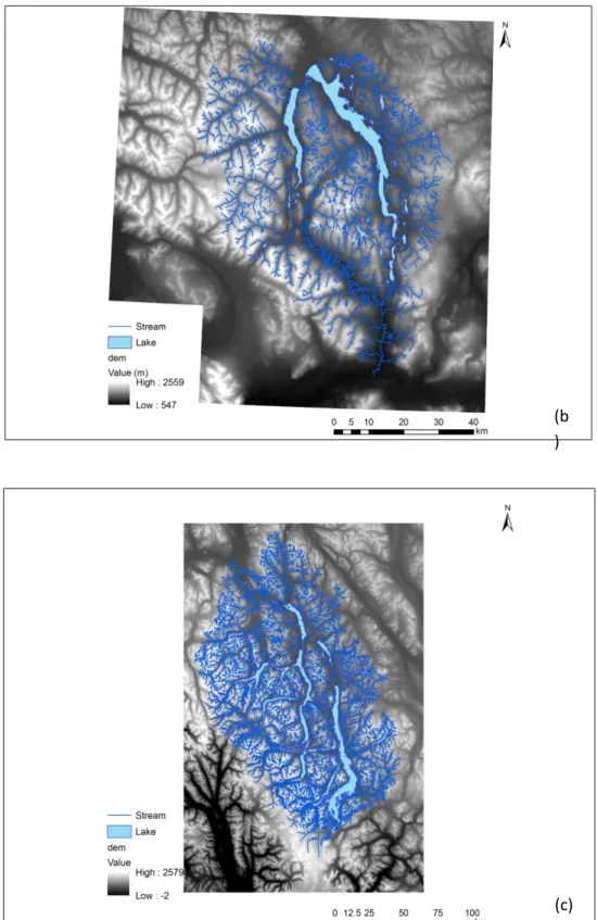
Figure 2.1 presents the DEM and the stream and lake networks of the Mayo, Aishihik and Upper Yukon watersheds. Note that DEMs cover larger areas than those of each watershed.

(27)

Figure 2.1 DEMs and stream and lake networks: (a) Mayo Watershed (b) Aishihik Watershed and (c) Upper Yukon River watershed.

(b )

(28)

Figure 2.1 illustrates that the each corrected stream and lake network is dense and complex with a high level of details.

Land cover

Initially, we explored various sources of data that could be used to define the required land cover map. Two sets of existing data were selected based on their coverage and standardized format. We built an initial land cover map based on the MODIS Canadian land cover map. This classification, dating back to 2005, was performed by the Canadian Remote Sensing Center (Natural Resources Canada) using MODIS satellite images. To our knowledge, this classification is the most recent that entirely covers Canada. It has a 250-m horizontal resolution and includes 39 different land cover classes. From a hydrological modelling point of view, there are too many land cover classes. Thus, we reduced the number of classes to 7 or 9 for the Upper Yukon River watershed. There is no need of having a large number of land cover classes as they will mostly end up having similar or identical parameter values. Table 2.1 presents the regrouped classes of the MODIS classification.

Second, we built a supplementary land cover map based on the Canadian 2000 CIRCA classification from Natural Resources Canada. This classification which covers the whole country was performed with Landsat images. When compared to the MODIS classification, the CIRCA classification has a better horizontal resolution (i.e., 30 m) which incidentally matches the DEM resolution. It includes 43 different land cover classes. Again to ensure a certain agreement with the MODIS classification, we reduced the number of classes to 7 or 9 for the Upper Yukon River watershed. Table 2.2 presents the regrouped classes for the CIRCA classification.

(29)

Table 2.2 Regrouped classes of the MODIS classification for the Mayo and Aishihik watersheds

MODIS classes Regrouped classes

Temperate or subpolar needle-leaved evergreen closed tree canopy (1) Evergreen Forest

Cold deciduous closed tree canopy (2) Deciduous Forest

Mixed needle-leaved evergreen – cold deciduous closed tree canopy (3) Mixed Forest

Mixed needle-leaved evergreen – cold deciduous closed young tree canopy (4) Mixed Forest

Mixed cold deciduous – needle-leaved evergreen closed tree canopy (5) Mixed Forest

Temperate or subpolar needle-leaved evergreen medium density, moss-shrub understory (6) Evergreen Forest

Temperate or subpolar needle-leaved evergreen medium density, lichen-shrub understory (7) Evergreen Forest Temperate or subpolar needle-leaved evergreen low density, shrub-moss understory (8) Evergreen Forest

Temperate or subpolar needle-leaved evergreen low density, lichen (rock) understory (9) Evergreen Forest

Temperate or subpolar needle-leaved evergreen low density, poorly drained (10) Evergreen Forest

Cold deciduous broad-leaved, low to medium density (11) Deciduous Forest

Cold deciduous broad-leaved, medium density, young regenerating (12) Deciduous Forest

Mixed needle-leaved evergreen – cold deciduous, low to medium density (13) Mixed Forest

Mixed cold deciduous - needle-leaved evergreen, low to medium density (14) Mixed Forest

Low regenerating young mixed cover (15) Mixed Forest

High-low shrub dominated (16) Shrub, Herb, lichen, bare soil, rock

Herb-shrub-bare cover (18) Shrub, Herb, lichen, bare soil, rock

Wetlands (19) Wetlands

Sparse needle-leaved evergreen, herb-shrub cover (20) Shrub, Herb, lichen, bare soil, rock

Polar grassland, herb-shrub (21) Shrub, Herb, lichen, bare soil, rock

Shrub-herb-lichen-bare (22) Shrub, Herb, lichen, bare soil, rock

Herb-shrub poorly drained (23) Shrub, Herb, lichen, bare soil, rock

Lichen-shrub-herb-bare soil (24) Shrub, Herb, lichen, bare soil, rock

Low vegetation cover (25) Shrub, Herb, lichen, bare soil, rock

High biomass cropland (27) Shrub, Herb, lichen, bare soil, rock

Lichen barren (30) Shrub, Herb, lichen, bare soil, rock

Lichen-spruce bog (32) Wetlands

Rock outcrops (33) Shrub, Herb, lichen, bare soil, rock

Recent burns (34) Burns

Old burns (35) Burns

Urban and Built-up (36) Urban

Water bodies (37) Water

Mixes of water and land (38) Water

(30)

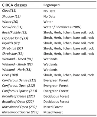
Table 2.3 Regrouped classes of the CIRCA classification for the Mayo and Aishihik Watersheds

CIRCA classes Regrouped

Cloud(11) No Data

Shadow (12) No Data

Water (20) Water

Snow/Ice (31) Water / Snow/Ice (uYRW)

Rock/Rubble (32) Shrub, Herb, lichen, bare soil, rock

Exposed land (33) Shrub, Herb, lichen, bare soil, rock

Bryoids (40) Shrub, Herb, lichen, bare soil, rock

Shrub tall (51) Shrub, Herb, lichen, bare soil, rock

Shrub low (52) Shrub, Herb, lichen, bare soil, rock

Wetland - Treed (81) Wetlands

Wetland - Shrub (82) Wetlands

Wetland - Herb (83) Wetlands

Herb (100) Shrub, Herb, lichen, bare soil, rock

Coniferous Dense (211) Evergreen Forest

Coniferous Open (212) Evergreen Forest

Coniferous Sparse (213) Evergreen Forest

Broadleaf Dense (221) Deciduous Forest

Broadleaf Open (222) Deciduous Forest

Mixedwood Open (232) Mixed Forest

Mixedwood Sparse (233) Mixed Forest

Regarding the two available products, we decided to use the land cover map build from the CIRCA classification since the 30-m resolution of the latter corresponded to that of the DEMs. Furthermore, for both watersheds, the No Data of the CICRA classification were corrected using the more recent MODIS classification (2005 versus 2000). This correction affected more the Aishihik Watershed because of a larger non-classified area on the CIRCA classification. Figure 2.2 shows the resulting land cover maps of the Mayo, Aishihik and Upper Yukon Watersheds. Also, for all watersheds, the stream and lake networks were superimposed on the original classification in order to properly match the water routing and the land cover. Note also that the Alaska National Land Cover Database classification was included to have a complete coverage of the Upper Yukon River watershed. Moreover, this latter

(31)

(a

(b )

(32)

Figure 2.2 Land cover maps: (a) Mayo, (b) Aishihik and (c) Upper Yukon River Watersheds.

It can be mentioned the Geomatics Yukon website offers other land cover products that focus mainly on forest resources. Namely, Vegetation and Vegetation Inventory products were not used to produce the land cover maps because they solely depict the presence or absence of forested areas and give information on tree species for the forest industry. From a hydrological modelling perspective, there is no need for a complete coverage of the area and the type of trees does not need to be as precise as that reported in the Vegetation Inventory. Indeed, ultimately the land cover classes will be regrouped

(33)

and Upper Yukon River Watershed; while there is no soil information for the Aishihik Watershed. That is why we have decided to look for other sources of information. Based on previous work performed in northern Quebec, there exists an alternative soil texture map covering Northern America at a 1-km resolution.

From a hydrological modelling perspective, HYDROTEL conceptualizes the soil profile as a series of different soil layers with constant hydrodynamics properties. When field measurements are unavailable, default values based on the work of Rawls and Brakensiek (1989) can be used, given basic soil texture information, namely percentages of sand, silt and clay.

The soil type maps developed for the Mayo, Aishihik and Upper Yukon River Watersheds are based on percentages of sand and clay available for three soil layers. These maps were derived from the work of Szeto et al. (2008) and they are based on the Soil Landscape of Canada V.2.2. It is the same data that were used as input data to the Canadian Land Surface Scheme (CLASS) of the Canadian Regional Climate Model. It is noteworthy that these maps do not provide any information on non-mineral land cover such as water, outcrops, and organic soils, as they cannot be related to any soil texture composition. The soil type maps were derived as follows.

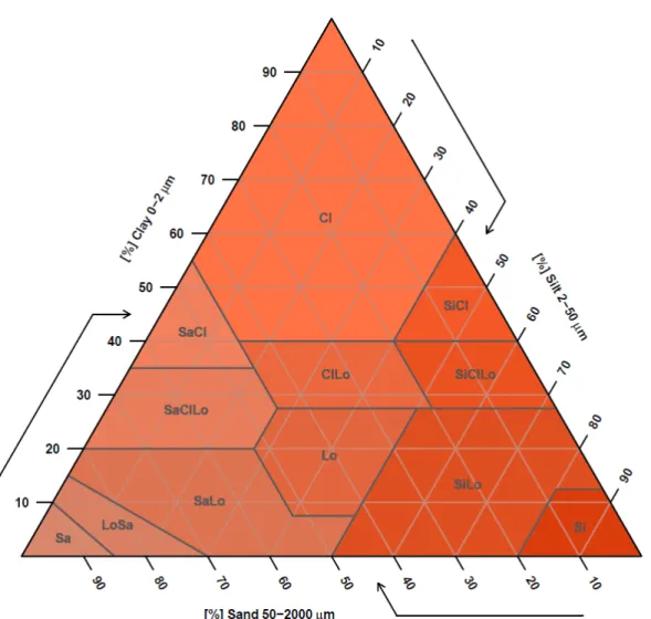
1. For each 1-km tile and soil horizon (0-10cm; 10-25cm; 25-375cm), the soil type was defined by percentages of sand, clay and silt based on the following soil texture triangle (Figure 2.3).

2. Development of a soil type map for the second soil layer (10-25cm). HYDROTEL allows for the use of a different soil type map for each soil layer required by the vertical water budget sub-model (BV3C). Given the coarse spatial resolution of the basic information, it was decided to use a unique soil type map valid for all three soil layers based on the information available for the second soil layer of the reference data. However, in the presence of a non-mineral soil type, the information available for layer one or layer three were used to substitute the non-mineral soil with the mineral soil information when available. Nonetheless, the resulting maps for all watersheds include non-mineral soils with default values for hydrodynamic properties.

3. The ensuing tiles of 1-km resolution were subdivided into 30-m tiles; that is the resolution of the DEMs.

(34)

Figure 2.3 Soil texture triangle (Moeys, 2009).

Abbreviations used within the triangle are: Cl : clay, SiCl : silty-clay, SaCl : sandy-clay, SiClLo : silty-clay-loam, ClLo : clay-loam, SaClLo : sandy-clay-loam, SiLo : silty-loam, Lo : loam, SaLo : sandy-loam, Si : silt, LoSa :

(35)

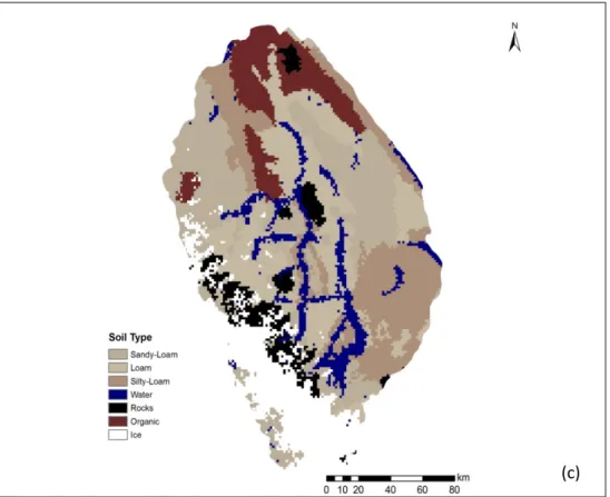
(a)

(36)

Figure 2.4 Soil type maps: of (a) Mayo, (b) Aishihik) and (c) Upper Yukon River Watersheds. As mentioned earlier, there exists in PHYSITEL a table relating the soil textures of various soil types developed by Rawls and Brakensiek (1989). It is noteworthy that non-mineral textures can be added to the existing table. Using the soil type map, PHYSITEL determines the dominant soil type of each RHHU. Using the hydrodynamic soil properties look-up table, HYDROTEL estimates the ensuing properties for each RHHU. For mineral soils, the hydrodynamic properties correspond to the default values described in the Rawls and Brakensiek (1989). For non-mineral soils, the hydrodynamic properties have to be determined. Similarly to the works of Jutras et al. (2009), these properties for clay were assigned to the

(37)

2.2.2. Watershed discretization using PHYSITEL

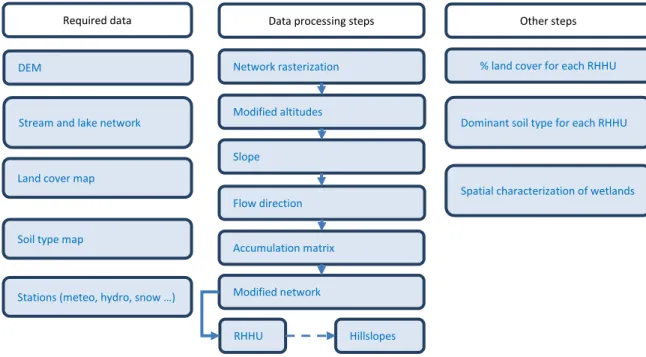
Using a DEM, a soil type map, a land cover map, and optionally a hydrographic network; PHYSITEL computes physiographic parameters for each RHHU. Namely, PHYSITEL determines the internal drainage structure (slopes and flow directions), watershed boundaries, sub-basin and hillslope boundaries, and hydrographic network. For each RHHU, PHYSITEL calculates the topographic index distribution and characterizes the dominant soil type, and percentages of different land covers. Because of standard data formats and universal data types, output data can be used for a wide range of distributed hydrological models. What differentiates PHYSITEL from most GISs are the following characteristics: (i) use of the D8-LTD algorithm of Orlandini et al. (2003) to compute the flow matrix, (iii) access to editing tools to modify the flow matrix and correct the stream and lake network, and (iii) optional use of a hydrographic network to determine the internal drainage structure of a watershed. PHYSITEL can be described as a step by step wizard that guides and helps the user to proceed to watershed discretization. Figure 2.5 summarizes the PHYSITEL input data and data processing.

Figure 2.5 PHYSITEL – Input data and data processing.

Required data

DEM

Stream and lake network

Land cover map

Soil type map

Data processing steps

Network rasterization Modified altitudes Slope Flow direction Accumulation matrix Modified network RHHU Other steps

Stations (meteo, hydro, snow …)

% land cover for each RHHU

Dominant soil type for each RHHU

Spatial characterization of wetlands

(38)

The different steps of data processing can be described as follows:

1. After correcting the stream and lake network, the vector and polygon network is converted into a raster file.

2. The rasterized network is burned on the DEM to facilitate water routing to and through the network.

3. Using the DEM, PHYSITEL calculates the slope of each cell or tile based on the north-south and east-west transects of each cell.

4. Again for each cell composing the DEM, PHYSITEL calculates the flow direction matrix using the D8-LTD algorithm of Orlandini et al. (2003).

5. Based on the flow direction of each cell, PHYSITEL determines the flow accumulation matrix that is for each cell the number of upstream drained cell. For a given outlet, such matrix regroups all the drained upstream cells.

6. Depending on the complexity of the streams and lakes, PHYSITEL allows for the derivation of the hydrologic network using either one of the following options. First, the final network can be identical to the imported and rasterized network. Second, the user can specify a threshold that determines the inclusion or not of a cell into the final network based on the number of upstream drained cells.

7. PHYSITEL identifies the drained cells of each stream or lake to determine the RHHUs. PHYSITEL subdivides the RHHUs into hillslopes in order to have a better representation of the terrain mean slope and mean aspect.

(39)

network for the hydrological forecasting system. This way, a reduced number of streams and lakes will be supported by a more reasonable number of RHHUs.

Figures 2.6 and 2.7 present the final hydrographic networks and hillslope subdivisions for the Mayo, Aishihik and Upper Yukon River Watersheds.

(a)

(40)

Figure 2.6 Modelled hydrological networks for: (a) Mayo, (b) Aishihik and (c) Upper Yukon River Watersheds.

(c)

(41)

Figure 2.7 RHHU / Hillslope delineation of Mayo (a) Aishihik (b) and (c) Upper Yukon River Watersheds. The distinctive color pattern for the Upper Yukon River Watershed relates to the use of a newer version of PHYSITEL to perform watershed discretization. This newer version allows for larger watershed to be discretized.

Table 2.4 summarizes the modelling characteristics of the discretized Mayo, Aishihik and Upper Yukon River Watersheds.

(b)

(42)

Table 2.4 Modelling characteristics of the discretized Mayo, Aishihik and Upper Yukon River Watersheds.

Mayo Aishihik Upper Yukon River Number of RHHUs as Hillslope 838 1737 1960 Mean RHHU area 3.19km² 2.63km² 10.39km² Number of stream and lakes 311 668 702

The RHHU mean area for the Upper Yukon is larger than those for Mayo and Aishihik. The reason is simply related to the number of RRHUs that are used to represent a larger watershed. The number of RHHUs remains under 2000 in order to have an acceptable computational time for simulation and data assimilation for each watershed. It is noteworthy that the data assimilation scheme developed by NCE limits the maximum number of RHHUs to 2000.

The final step corresponds to the identification of nearby meteorological stations own by Environment and Climate Change Canada and to the downloading of historical and available data (temperature and precipitations).

2.2.3. HYDROTEL integration and hydrological simulation

Integration of the Mayo, Aishihik and Upper Yukon River Watersheds to HYDROTEL is supported by the different files created by PHYSITEL; while simulations are driven by hydrometeorological data. Model calibration requires observed stream flows or reconstructed reservoir/lake inflows and any other relevant state variables (e.g., SWE). From a hydrological modelling perspective, HYDROTEL is a semi-distributed model; that is based on one-dimensional and two dimensional governing equations. Given the available meteorological data for the studied watersheds, the model runs on a daily time step. The

(43)

within or near the studied watersheds would be welcome and increase the quality of the hydrological simulations. This database also includes snow survey measurements (snow height and SWE) that can be assimilated during the production of the hydrological forecasts.

Figure 2.8 and Table 2.5 present the different hydrometeorological stations and snow survey sites for all three watersheds.

(44)

(b )

(45)

Mayo

NAME OF THE STATION PROVINCE STATION # DATA START END TIME STEP TYPE DATA FROM

DRURY CREEK YT 2100460 T. AND P. 1970 2009 DAILY MANUAL MSC

ELSA YT 2100500 T. AND P. 1948 1989 DAILY MANUAL MSC

KENO HILL YT 2100677 T. AND P. 1974 1982 DAILY MANUAL MSC

MAYO A YT 2100700 T. AND P. 1924 2013 HOURLY AND DAILY AUTO. AND MANUAL MSC MAYO A YT 2100701 T. AND P. 2013 2017 HOURLY AND DAILY AUTO. AND MANUAL MSC

MOOSE CREEK YT 2100746 T. AND P. 1972 1975 DAILY MANUAL MSC

RUSSELL CREEK YT 2100942 T. AND P. 1989 1993 DAILY MANUAL MSC

STEWART CROSSING YT 2101030 T. AND P. 1953 2008 DAILY MANUAL MSC

STEWART CROSSING TOWER YT 2101031 T. AND P. 1976 1976 DAILY MANUAL MSC

TWO PETE CREEK YT 2101138 T. AND P. 1979 1984 DAILY MANUAL MSC

MAYOMET YT MAYOMET T. AND P. 2017 2017 HOURLY AND DAILY AUTO. AND MANUAL YEC-YNC

Aishihik

MULE CREEK BC 1205248 T. AND P. 1970 1986 DAILY MANUAL MSC

WINDY CRAGGY BC 120HRNP T. AND P. 1987 1990 DAILY MANUAL MSC

AISHIHIK A YT 2100100 T. AND P. 1943 1966 HOURLY AND DAILY MANUAL MSC BLANCHARD RIVER YT 2100163 T. AND P. 1986 2012 DAILY AUTOMATIC MSC

BRAEBURN YT 2100167 T. AND P. 1974 1995 DAILY MANUAL MSC

BURWASH YT 2100179 T. AND P. 1993 2004 HOURLY AND DAILY AUTOMATIC MSC BURWASH A YT 2100181 T. AND P. 2011 2017 HOURLY AND DAILY AUTO. AND MANUAL MSC BURWASH A YT 2100182 T. AND P. 1966 2015 HOURLY AND DAILY AUTOMATIC MSC BURWASH AIRPORT AUTO BC YT 2100184 T. AND P. 2013 2017 HOURLY AND DAILY AUTOMATIC MSC

CARMACKS YT 2100300 T. AND P. 1963 2008 DAILY MANUAL MSC

CARMACKS CS YT 2100301 T. AND P. 1999 2017 HOURLY AND DAILY AUTOMATIC MSC

CARMACKS TOWER YT 2100302 T. AND P. 1974 1976 DAILY MANUAL MSC

DESTRUCTION BAY YT 2100418 T. AND P. 1975 1984 DAILY MANUAL MSC

DEZADEASH YT 2100430 T. AND P. 1974 1986 DAILY MANUAL MSC

HAINES APPS #4 YT 2100627 T. AND P. 1969 1971 DAILY MANUAL MSC

HAINES JUNCTION YT 2100630 T. AND P. 1944 2017 HOURLY AND DAILY AUTOMATIC MSC HAINES JUNCTION YTG YT 2100631 T. AND P. 1985 2008 DAILY MANUAL MSC

KLUANE LAKE YT 2100680 T. AND P. 1946 1983 DAILY MANUAL MSC

MINTO YT 2100744 T. AND P. 1974 1974 DAILY MANUAL MSC

OTTER FALLS NCPC YT 2100840 T. AND P. 1980 2015 DAILY MANUAL MSC

PAINT MOUNTAIN TOWER YT 2100850 T. AND P. 1976 1976 DAILY MANUAL MSC

(46)

GLADSTONE MET STATION YT GLADMET T. AND P. 2009 2012 HOURLY AUTOMATIC YEC AISHIHIK MET STATION YT AISHMET T. AND P. 2017 2017 AUTOMATIC YEC-YNC

Upper Yukon River

ATLIN BC 1200560 T. AND P. 1899 2017 DAILY MANUAL MSC

BENNET BC 1200847 T. AND P. 1972 1974 DAILY MANUAL MSC

GRAHAM INLET BC 1203255 T. AND P. 1973 2011 DAILY MANUAL MSC

LINDEMAN CITY BC 1204632 T. AND P. 1968 1981 DAILY MANUAL MSC

NAKONAKE RIVER BC 1205295 T. AND P. 1956 1956 DAILY MANUAL MSC

FRASER CAMP BC 120C036 T. AND P. 1980 2008 DAILY MANUAL MSC

ANNIE LAKE ROBINSON YT 2100115 T. AND P. 1976 2006 DAILY MANUAL MSC

BRAEBURN YT 2100167 T. AND P. 1974 1995 DAILY MANUAL MSC

BRYN NYRDDIN FARM YT 2100174 T. AND P. 1988 1996 DAILY AUTOMATIC MSC

CARCROSS YT 2100200 T. AND P. 1907 2008 DAILY MANUAL MSC

FISH LAKE ROAD YT 2100535 T. AND P. 1988 1989 DAILY MANUAL MSC

GOLDEN HORN YT 2100615 T. AND P. 1989 1994 DAILY MANUAL MSC

HAECKEL HILL TOWER YT 2100620 T. AND P. 1974 1976 DAILY MANUAL MSC

JOHNSONS CROSSING YT 2100670 T. AND P. 1963 1995 DAILY MANUAL MSC

MARSH LAKE YT 2100698 T. AND P. 1994 2002 DAILY MANUAL MSC

MAYO ROAD YT 2100709 T. AND P. 1983 2016 DAILY MANUAL MSC

NEW IMPERIAL YT 2100765 T. AND P. 1968 1969 DAILY MANUAL MSC

PORTER CREEK WAHL YT 2100907 T. AND P. 1989 2005 DAILY MANUAL MSC

QUIET LAKE YT 2100910 T. AND P. 1966 1992 DAILY MANUAL MSC

(47)

TULSEQUAH BC 1208295 T. AND P. 1964 1966 DAILY MANUAL MSC

MORLEY RIVER YT 2100750 T. AND P. 1984 1989 DAILY MANUAL MSC

FANTAIL LOWER BC FANTLOW T. AND P. 2012 2017 HOURLY AUTOMATIC YRC-YEC FANTAIL UPPER BC FANTUPP T. AND P. 2012 2017 HOURLY AUTOMATIC YRC-YEC LLEWELLYN LOWER BC LLEWLOW T. AND P. 2013 2017 HOURLY AUTOMATIC YRC-YEC LLEWELLYN UPPER BC LLEWUPP T. AND P. 2013 2016 HOURLY AUTOMATIC YRC-YEC

WHEATON YT WHEATON T. AND P. 2014 2017 HOURLY AUTOMATIC YRC-YEC

For the three studied watersheds, all meteorological stations own by Environment Canada or YEC with measurements from the 20th

century and located within a 200-km radius are included in Table 2.5. For the forecasting system, only stations with current measurements are relevant. Also new or existing stations not related to Meteorological Service of Canada could be added to the previous list. Note that for the Mayo, Aishihik, and Upper Yukon River Watersheds, there are 2, 5 and 9 operational stations, respectively, including recently added meteorological station in Aishihik and Mayo Watersheds. During the calibration process, only the operational stations were considered since the forecasting system. This consideration prevents the use of removed or closed stations for model calibration, since the forecasting system would not be able to use them anyway. Note that the Upper Fantail station was removed from the Upper Yukon River Watershed and relocated within the boundaries of the Mayo Watershed which only had one operational meteorological station. It is noteworthy that operational stations can be located beyond watershed boundaries, but their monitored conditions may note represent those occurring within the watershed boundaries.

(48)

Table 2.6 Hydrometric stations of the Mayo, Aishihik and Upper Yukon River Watersheds.

Mayo

NAME OF THE STATION PROVINCE STATION # DATA START END OPERATION TYPE DATA FROM MAYO LAKE NEAR THE OUTLET YT 09DC005 WATER LEVEL 1979 2017 CONTINUOUS 5 MINUTES WSC MAYO RIVER NEAR MAYO YT 09DC001 FLOW 1945 1951 DISCONTINUOUS DAILY WSC WAREHAM LAKE AT HEADGATE YT 09DC004 WATER LEVEL 1979 2000 CONTINUOUS DAILY WSC MAYO LAKE AT THE OUTLET YT YECMAYO FLOW 1979 2017 CONTINUOUS 5 MINUTES YEC INFLOW TO MAYO LAKE YT 0000003 FLOW 1979 2017 CONTINUOUS DAILY YEC Aishihik

NAME OF THE STATION PROVINCE STATION # DATA START END OPERATION TYPE DATA FROM

AISHIHIK RIVER NEAR WHITEHORSE YT 08AA001 FLOW 1950 1986 Contiuous DAILY WSC AISHIHIK LAKE NEAR WHITEHORSE YT 08AA005 WATER LEVEL 1972 2017 Contiuous 5 MINUTES WSC AISHIHIK RIVER BELOW AISHIHIK LAKE YT 08AA010 FLOW AND WATER

LEVEL 1980 2017 Contiuous 5 MINUTES WSC GILTANA CREEK NEAR THE MOUTH YT 08AA009 FLOW AND WATER

LEVEL 1980 2017 Contiuous 5 MINUTES WSC SEKULMUN LAKE NEAR WHITEHORSE YT 08AA007 WATER LEVEL 1980 2017 Contiuous 5 MINUTES WSC SEKULMUN RIVER AT OUTLET OF SEKULMUN LAKE YT 08AA008 FLOW AND WATER

LEVEL 1981 2017 Contiuous 5 MINUTES WSC WEST AISHIHIK RIVER NEAR THE MOUTH YT 08AA011 FLOW 1995 2000 Contiuous DAILY WSC AISHIHIK LAKE NEAR AISHIHIK YT 08AA012 WATER LEVEL 1995 2015 Contiuous 5 MINUTES WSC

(49)

noteworthy that stations that only monitored water levels cannot be used, since HYDROTEL does not simulate reservoir or lake levels. For the forecasting system, some stations will have no use (i.e., non-operational stations, water level stations). Also for Aishihik, ISAAC CREEK 1 and 2 were not used since they have very limited measurements and are located upstream of the Sekulmun River station.

Table 2.7 Snow survey sites for the Mayo, Aishihik and Upper Yukon River Watersheds.

Mayo

NAME OF THE STATION PROVINCE COURSE ID # DATA START END OPERATION TYPE DATA FROM

CALUMET YT 09DD-SC01 DEPTH / SWE 1975 2017 UP TO 5 days / Year MANUAL Environment Yukon EDWARDS LAKE YT 09DD-SC02 DEPTH / SWE 1987 2016 UP TO 5 days / Year MANUAL Environment Yukon MAYO AIRPORT A YT 09DC-SC01A DEPTH / SWE 1968 2017 UP TO 5 days / Year MANUAL Environment Yukon MAYO AIRPORT B YT 09DC-SC01B DEPTH / SWE 1987 2017 UP TO 5 days / Year MANUAL Environment Yukon Aishihik

NAME OF THE STATION PROVINCE COURSE ID # DATA START END OPERATION TYPE DATA FROM

AISHIHIK LAKE YT 08AA-SC03 DEPTH / SWE 1994 2017 UP TO 5 days / Year MANUAL Environment Yukon CANYON LAKE YT 08AA-SC01 DEPTH / SWE 1975 2017 UP TO 5 days / Year MANUAL Environment Yukon MACINTOSH YT 09CA-SC02 DEPTH / SWE 1976 2016 UP TO 5 days / Year MANUAL Environment Yukon AISHMET YT AISHMET DEPTH / SWE 2017 2017 UP TO 5 days / Year AUTOMATIC Yukon College AISRS01 YT AISRS01 DEPTH / SWE 2017 2017 UP TO 5 days / Year MANUAL Yukon College AISRS02 YT AISRS02 DEPTH / SWE 2017 2017 UP TO 5 days / Year MANUAL Yukon College

Upper Yukon River

NAME OF THE STATION PROVINCE COURSE ID # DATA START END OPERATION TYPE DATA FROM WHITEHORSE AIRPORT YT 09AB-SC2 DEPTH / SWE 2006 2017 UP TO 5 days / Year MANUAL Environment Yukon MT. MCINTYRE (B) YT 09AB-SC1B DEPTH / SWE 2006 2017 UP TO 5 days / Year MANUAL Environment Yukon TAGISH YT 09AA-SC1 DEPTH / SWE 2006 2017 UP TO 5 days / Year MANUAL Environment Yukon MONTANA MOUNTAIN YT 09AA-SC2 DEPTH / SWE 2006 2017 UP TO 5 days / Year MANUAL Environment Yukon

(50)

EAGLECREST AL 0034J03 DEPTH / SWE 2006 2017 UP TO 5 days / Year MANUAL USDA NRCS MEADOW CREEK YT 09AD-SC1 DEPTH / SWE 2006 2017 UP TO 5 days / Year MANUAL Energy Mines and

Ressources Yukon FANTAIL LOWER BC FANTLOW DEPTH / SWE 2012 2017 HOURLY AUTOMATIC Yukon College FANTAIL UPPER BC FANTUPP DEPTH / SWE 2012 2017 HOURLY AUTOMATIC Yukon College LLEWELLYN LOWER BC LLEWLOW DEPTH / SWE 2013 2017 HOURLY AUTOMATIC Yukon College LLEWELLYN UPPER BC LLEWUPP DEPTH / SWE 2013 2016 HOURLY AUTOMATIC Yukon College WHEATON YT WHEATON DEPTH / SWE 2014 2017 HOURLY AUTOMATIC Yukon College

Table 2 introduces the different snow courses for the three watersheds and those snow stations with snow height and snow SWE measurements. Note that the Upper Fantail station was removed from the Upper Yukon River Watershed and relocated within the Mayo Watershed. For the Upper Yukon River Watershed, snow courses prior to 2006 were not included in the database.

The resulting hydrometeorological database for the Mayo, Aishihik and Upper Yukon River Watersheds were then integrated into HYDROTEL. Figure 2.9 presents a screenshot of the three watersheds within the HYDROTEL graphical user interface while Figure 2.10 gives an example of the workspace window for the Aishihik Watershed. The portion of the Aishihik Watershed displayed in beige represents the simulated area and the grey portion, the non-simulated area. It also shows the information menu on the right and the action menu at the top.

(51)

Figure 2.9 Mayo, Aishihik and Upper Yukon River Watersheds displayed using the HYDROTEL graphical user interface.

(52)

HYDROTEL models the major physical processes of the water budget using sub-models that include different algorithms or simulation options. As shown in Table 2.8, each sub-model generally offers more than one simulation options.

Table 2.8 HYDROTEL sub-model and simulation Options

Water budget component (sub-model) Simulation options 1 Interpolation of meteorological data 1.1 Thiessen polygons

1.2 Weighted mean of nearest three stations

2 Snow accumulation and melt 2.1 Mixed (degree-day) energy-budget method

2.2 Multi-layer model* 3 Soil temperature and soil freezing 3.1 Rankinen

3.2 Thorsen

4 Glacier dynamics 4.1 Glacier model*

5 Potential evapotranspiration 5.1 Thornthwaite 5.2 Linacre 5.3 Penman 5.4 Priestley-Taylor 5.5 Hydro-Québec

5.6 Penman-Monteith

6 Vertical water budget 6.1 BV3C

6.2 CEQUEAU (modified) 7 Overland water routing 7.1 Kinematic wave equation

8 Channel water routing 8.1 Kinematic wave equation

8.2 Diffusive wave equation

* Model and simulation option to be developed as part of the current project.

In the above table, the bold face nouns represent the simulation option used for hydrological simulation.

(53)

everything is identical for each one of those units, as the hydraulic characteristics on each unit depend on soil type, which are different from unit to another, for instance.

Since model calibration for the Aishihik and Mayo Watersheds relies heavily on the reconstructed reservoir/lake inflows, it seems important to describe the methodology and the equation currently used to determine them.

The general water budget equation for a reservoir or a lake can be expressed as follows:

∆𝑉𝑉 = 𝐼𝐼𝐼𝐼 + 𝑃𝑃 − 𝐸𝐸 − 𝑄𝑄𝑜𝑜𝑜𝑜𝑜𝑜 (1)

Where:

∆𝑉𝑉 = variation of lake or reservoir volume (V) between time (j-1) and (j) (m³/s); 𝐼𝐼𝐼𝐼 = sum of inflows from upstream rivers and surrounding hillslopes;

𝑃𝑃 = precipitation on the surface of the lake or reservoir; 𝐸𝐸 = evaporation from the surface of the lake or reservoir; 𝑄𝑄𝑜𝑜𝑜𝑜𝑜𝑜 = sum of the entire lake or reservoir outflows.

For both Aishihik and Mayo, 𝑃𝑃 and 𝐸𝐸 were not considered since they can be assumed to be similar over time. Only ∆𝑉𝑉 and 𝑄𝑄𝑜𝑜𝑜𝑜𝑜𝑜 need to be determined to estimate 𝐼𝐼𝐼𝐼 as the total inflow.

For both watersheds, we adopted a calculation procedure based on the three-day water level average, thus:

∆𝑉𝑉 = 𝑉𝑉𝑗𝑗− 𝑉𝑉𝑗𝑗−1 (2)

For Aishihik Lake the general volume calculation is as follows: When L < 915

𝑉𝑉 = −38627.31𝐿𝐿6_{+ 678170.61𝐿𝐿}5_{− 3270008.00𝐿𝐿}4_{+ 6352008.56𝐿𝐿}3_{− 3111511.38𝐿𝐿}2_{+ 134383853.50} (3) When L >= 915

(54)

𝑉𝑉 = −50827494.83𝐿𝐿4_{+ 731085628.63𝐿𝐿}3_{− 3932429415.76𝐿𝐿}2_{+ 9545583654.41𝐿𝐿 − 8448705648.59} (4) Where 𝐿𝐿 represents the water level of water recorded at Aishihik Lake near Whitehorse hydrometric station (08AA005). Note that the record at the (08AA005) station must be cumulated to the reference water level (911.565) in order to have the proper water level for the volume calculation in Equations (3) and (4). The results of Equation (4) need to be multiplied by 3600 to get a daily volume.

For Mayo Lake the general volume calculation is as follows:

𝑉𝑉 =_0.00003814(𝐿𝐿−660) *3600 (5)

Here 𝐿𝐿 represents the water recorded at the Mayo Lake near the outlet hydrometric station (09DC005). Note that the record at the (09DC005) station must be cumulated to the reference water level (662.337) in order to have the proper water level for the volume calculation in Equation (5). To calculate volume variations based on the average water level of the last three days, 𝐿𝐿 in Equations (3) to (5) are calculated as follows:

𝐿𝐿 =𝐿𝐿𝑗𝑗+𝐿𝐿𝑗𝑗−1+𝐿𝐿𝑗𝑗−2

3 (6)

Where:

𝐿𝐿𝑗𝑗 , 𝐿𝐿𝑗𝑗−1 and 𝐿𝐿𝑗𝑗−2 represent the daily mean water level at the reference hydrometric station for the

current day (j), previous day (j-1) and two day prior (j-2).

Before determining the total inflow (𝐼𝐼𝐼𝐼) in Equation (1), the volume variation must be divided by 86400 s/day to get the flow units (m³/s).

(55)

𝑄𝑄08𝐴𝐴𝐴𝐴009= The average daily flow at the Giltana Creek near the mouth hydrometric station

(08AA009).

To calculate the most accurate lake outflow, we need to subtract the Giltana Creek (08AA009) flow from the Aishihik River measurements since the (08AA010) hydrometric station is located downstream of both Aishihik Lake and Giltana Creek and is the closest flow measurement downstream of the Lake. To determine 𝑄𝑄𝑜𝑜𝑜𝑜𝑜𝑜 for Mayo Lake, we use the following equation:

𝑄𝑄𝑜𝑜𝑜𝑜𝑜𝑜 = 𝑄𝑄𝑌𝑌𝑌𝑌𝑌𝑌𝑌𝑌𝐴𝐴𝑌𝑌𝑌𝑌 (8)

Where:

𝑄𝑄𝑌𝑌𝑌𝑌𝑌𝑌𝑌𝑌𝐴𝐴𝑌𝑌𝑌𝑌= The average daily flow measurement made by YEC at the outlet of the Mayo Lake

facility.

As the volume variation ∆𝑉𝑉 is calculated between the current day (j) and the previous day (j-1) the 𝑄𝑄𝑜𝑜𝑜𝑜𝑜𝑜 value in Equation (1) must be calculated as follows:

𝑄𝑄𝑜𝑜𝑜𝑜𝑜𝑜 = 𝑄𝑄𝑜𝑜𝑜𝑜𝑜𝑜,𝑗𝑗+𝑄𝑄₂𝑜𝑜𝑜𝑜𝑜𝑜,𝑗𝑗−1 (9)

Where 𝑄𝑄𝑜𝑜𝑜𝑜𝑜𝑜,𝑗𝑗 and 𝑄𝑄𝑜𝑜𝑜𝑜𝑜𝑜,𝑗𝑗−1 represent for both watersheds the outflow (Equations 6 & 7) for the current

day (j) and the previous day (j-1).

For both watersheds, a particular case must be addressed to ensure proper calculation of the total daily average inflow.

For Aishihik, measurements at the Giltana Creek hydrometric station (08AA009) are missing sometimes. Under such circumstances, a precise procedure was developed by YEC to correct flow measurements at the Aishihik River station (08AA010) and it can be accounted for using a specific equation.

When 𝑄𝑄08𝐴𝐴𝐴𝐴009 is missing, the correction applied to the 𝑄𝑄08𝐴𝐴𝐴𝐴010 measured flow is given by the

(56)

𝑄𝑄08𝐴𝐴𝐴𝐴010= 𝑚𝑚(𝑚𝑚𝑜𝑜𝑚𝑚𝑜𝑜ℎ)𝑄𝑄08𝐴𝐴𝐴𝐴010+ 𝑏𝑏(𝑚𝑚𝑜𝑜𝑚𝑚𝑜𝑜ℎ) (10)

Where 𝑚𝑚(𝑚𝑚𝑜𝑜𝑚𝑚𝑜𝑜ℎ) and 𝑏𝑏(𝑚𝑚𝑜𝑜𝑚𝑚𝑜𝑜ℎ) represent the slope and the intercept of the linear regression equation

calculated for every month of the year. The monthly values of 𝑚𝑚 and 𝑏𝑏 are introduced in Table 2.9. Table 2.9 Monthly values of slope and intercept of the linear regression equation to estimate the Aishihik River station (08AA010) flows when measurements at the Giltana Creek hydrometric station (08AA009) are missing.

Month m b 1 0.995 -0.048 2 0.997 -0.046 3 0.999 -0.055 4 0.990 -0.102 5 0.869 -1.070 6 0.822 -0.576 7 0.980 -0.592 8 0.957 -0.193 9 0.959 -0.352 10 0.978 -0.416 11 0.995 -0.266 12 0.992 -0.093

It is important to highlight that for both watersheds, the estimated total inflows may result in a negative value. This is known as a false negative value, because the water budget equation assumes a

(57)

For Aishihik Lake:

When 𝐼𝐼𝐼𝐼 < 0.0m³/s then 𝐼𝐼𝐼𝐼 = 0.01 𝑜𝑜𝑜𝑜 𝑄𝑄08𝐴𝐴𝐴𝐴008

For Mayo Lake:

When 𝐼𝐼𝐼𝐼 < 0.0m³/s then 𝐼𝐼𝐼𝐼 = 0.01

The nominal values for Aishihik Lake and Mayo Lake correspond to the minimum positive inflow calculated for the entire historical period available.

Throughout the calibration procedure of HYDROTEL, model performance with respect to corroborating with measured flows or reconstructed inflows was evaluated using different criteria.

1. A visual inspection of the graphical representation of observed and simulated flows; 2. The Nash-Sutcliffe criterion calculated with the following equation:

𝐼𝐼𝑁𝑁 = 1 − ∑𝑛𝑛𝑠𝑠=1(𝑄𝑄𝑜𝑜𝑜𝑜𝑜𝑜−𝑄𝑄𝑜𝑜𝑠𝑠𝑠𝑠)2 ∑𝑛𝑛𝑠𝑠=1�𝑄𝑄𝑜𝑜𝑜𝑜𝑜𝑜−𝑄𝑄𝑜𝑜𝑜𝑜𝑜𝑜,𝑠𝑠𝑚𝑚𝑚𝑚𝑛𝑛�2

(11) Where 𝑄𝑄𝑜𝑜𝑜𝑜𝑜𝑜 represents the observed flow or reconstructed inflow, 𝑄𝑄𝑜𝑜𝑠𝑠𝑚𝑚 the simulated flow or inflow,

𝑄𝑄𝑜𝑜𝑜𝑜𝑜𝑜,𝑚𝑚𝑚𝑚𝑚𝑚𝑚𝑚 the mean observed flow or reconstructed inflow from day 1 to (n) number of days (daily

time step).

The value of the criterion ranges from (-∞ to 1.0) where one (1) represents the optimum. This criterion evaluates the amplitude and the synchronism between observed and simulated flows or inflows. Generally, this criterion is highly influenced by the presence and representation of the peak freshet that makes it less adapted for a long low flow period;

3. The observed and simulated annual runoff (water volume / watershed area) can be used to compare water volumes based on the following equation:

𝑅𝑅𝑅𝑅𝑅𝑅𝑜𝑜𝑅𝑅𝑅𝑅𝑦𝑦𝑚𝑚𝑚𝑚𝑦𝑦 = ∑ (𝑄𝑄 𝑥𝑥 𝑌𝑌𝑌𝑌𝐶𝐶𝐶𝐶) 𝑛𝑛

𝑠𝑠=1

(58)

Where 𝑅𝑅𝑅𝑅𝑅𝑅𝑜𝑜𝑅𝑅𝑅𝑅𝑦𝑦𝑚𝑚𝑚𝑚𝑦𝑦 represents the annual runoff expressed in (mm), 𝑄𝑄 the observed or simulated flow

or inflow (m³/s), 𝐴𝐴𝑅𝑅𝐸𝐸𝐴𝐴 the drainage area upstream of the comparison site (km²) and CONV a conversion factor to respect the proper unit (mm) of the resulting annual runoff;

4. The PBIAIS criterion (bias percentage) that is calculated with the following equation: 𝑃𝑃𝑃𝑃𝐼𝐼𝐴𝐴𝐼𝐼𝑁𝑁 =∑𝑛𝑛𝑠𝑠=1(𝑄𝑄𝑜𝑜𝑠𝑠𝑠𝑠−𝑄𝑄𝑜𝑜𝑜𝑜𝑜𝑜)

∑𝑛𝑛𝑠𝑠=1𝑄𝑄𝑜𝑜𝑜𝑜𝑜𝑜 𝑥𝑥 100 (13)

This criterion, expressed in (%), can be used to quantify the bias between simulated and observed values. The value of the criterion varies between (-∞ to +∞) where zero (0) is the optimum;

5. Root mean square error (RMSE) that can be calculated as follow: 𝑅𝑅𝑅𝑅𝑁𝑁𝐸𝐸 = �∑𝑛𝑛𝑠𝑠=1(𝑄𝑄𝑜𝑜𝑜𝑜𝑜𝑜−𝑄𝑄𝑜𝑜𝑠𝑠𝑠𝑠)2

𝑚𝑚 (14)

The resulting value of this criterion varies between (0 to +∞) where zero (0) is the optimum. This criterion expressed in m³/s for flows or inflows, assesses the general agreement between observed and simulated flows or inflows. Essentially this criterion is influenced by the largest discrepancies.

Calibration of HYDROTEL was first performed on the Aishihik Watershed using flows measured at the Sekulmun River at the outlet of the Sekulmun Lake hydrometric station (08AA008) and reconstructed inflows for Aishihik Lake. Secondly, the model was calibrated on the Mayo Watershed using the reconstructed inflows to Mayo Lake. Finally, a first calibration was performed for the Upper Yukon River Watershed using the flows recorded at the Yukon River at Whitehorse hydrometric station (09AB001). Note that at this stage of the project, we have performed a spatial calibration on the Aishihik Watershed with specific model calibration parameters for the entire Sekulmun River

(59)

The model calibration and the development of the data assimilation procedure for the Aishihik watershed were based on the aforementioned methodology used to reconstruct inflows (i.e., Aishihik Lake). An updated version of the water level/lake water volume relationship (Equations 3 and 4) was proposed mid November 2017. Throughout the calibration process, the Sekulmun River flows were used as inflows for cases where negative reconstructed inflows were obtained. During the first year of the project, it was decided instead that a nominal value would be used to correct the negative reconstructed inflows. As mentioned before, the calibration period ranges from 01/01/2010 to 31/12/2016. Figure 2.11 and Table 2.10 present the calibration results.

0 5 10 15 20 25 30 35 40 45 20 10- 01-01 20 10- 04-01 20 10- 07-01 20 10-01 20 11- 01-01 20 11- 04-01 20 11- 07-01 20 11- 10-01 20 12- 01-01 20 12- 04-01 20 12- 07-01 20 12- 10-01 20 13- 01-01 20 13- 04-01 20 13- 07-01 20 13- 10-01 20 14- 01-01 20 14- 04-01 20 14- 07-01 20 14- 10-01 20 15- 01-01 20 15- 04-01 20 15- 07-01 20 15- 10-01 20 16- 01-01 20 16- 04-01 20 16- 07-01 20 16- 10-01 Str ea m flo w s ( m³ /s) Date

Comparison of measured and simulated streamflows (Sekulmun River 2010-01-01 to 2016-12-31)

Measured Simulated