3D IMAGING OF INDIVIDUAL PARTICLES: A REVIEW
E
RICP
IRARDGeMMe-Georesources and GeoImaging, Université de Liège, Sart Tilman, B 52, 4000 Liege, Belgium e-mail: [email protected]
(Received May 10, 2012; revised June 7, 2012; accepted June 8, 2012)
ABSTRACT
In recent years, impressive progress has been made in digital imaging and in particular in three dimensional visualisation and analysis of objects. This paper reviews the most recent literature on three dimensional imaging with a special attention to particulate systems analysis. After an introduction recalling some important concepts in spatial sampling and digital imaging, the paper reviews a series of techniques with a clear distinction between the surfometric and volumetric principles. The literature review is as broad as possible covering materials science as well as biology while keeping an eye on emerging technologies in optics and physics. The paper should be of interest to any scientist trying to picture particles in 3D with the best possible resolution for accurate size and shape estimation. Though several techniques are adequate for nanoscopic and microscopic particles, no special size limit has been considered while compiling the review.
Keywords: quantitative microscopy, particle size analysis, surfometry, tomography, volumetry.
INTRODUCTION
PARTICULATE SYSTEMS
CHARACTERIZATION
Particles, as considered in the scope of this paper, are mostly solid fragments loosely dispersed in a liquid or a gas. In some favourable cases they may even be particles dispersed in a host solid. These particles can have a wide range of sizes and shapes. They can also be made of highly variable molecular assemblages. Examples of particulate systems can be found in almost any field of science, ranging from clay particles to asteroids or from snowflakes to diamonds.
Traditionally particles have been characterised by simple physical principles that could easily be linked to their fundamental characteristics: size, shape or nature. For centuries, sizing of particles has been achieved by a simple test of the probability of passing through a mesh. But, even this simple test results in a complex interaction between the particle and the sieve that can hardly be interpreted in terms of size only. Meloy (1977) showed for example, that in well conducted sieving experiments, this probability is proportional to the cube of the elongation of the particle. But, we could as well show that for concave (hook shaped) particles this probability can tend towards… zero! Even though the nature of the particle does not seem to play a role in the probability of passing through a mesh, all practitioners know that
sieving is simply impossible with fragile materials and that the result of a sieving operation is always expressed in terms of weight fraction retained within a sieve. This means that any difference in density between the size fractions will induce a distribution hard to interpret in terms of size only.
PARTICLE IMAGING
Because of the intrinsic limitations of all methods based on physical principles (sieving, sedimentation, laser diffraction, etc.), the potential for imaging individual particles and measuring their geometrical characteristics has attracted wide attention. The very early trials based on hand drawings (Wadell, 1933) have given place to a whole range of digital imaging principles and a series of standards issued by the ISO committee on “Particle characterization including sieving” (ISO TC24/SC4) and more specifically its working group on “Image Analysis”. The current standard makes a distinction between the so-called Static Image Analysis (SIA) instruments and the Dynamic Image Analysis instruments (DIA). This distinction is unfortunate in the sense that it suggests that one technique could be more productive than the other when in fact the distinction bears on the way particles are shown to the imaging device. Static image analysers picture particles at rest on a plane, whereas dynamic image analysers picture them in a free falling situation. More essentially, the distinction between SIA and DIA stresses the fact that their
results both in terms of particle size and particle shape distribution cannot be compared. SIA instruments have their optical axis perpendicular to the resting plane which means that the smallest dimension or thickness (c) cannot be captured whereas both the largest diameter or length (a) and the intermediate diameter or width (b) can be properly measured.
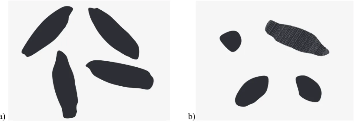
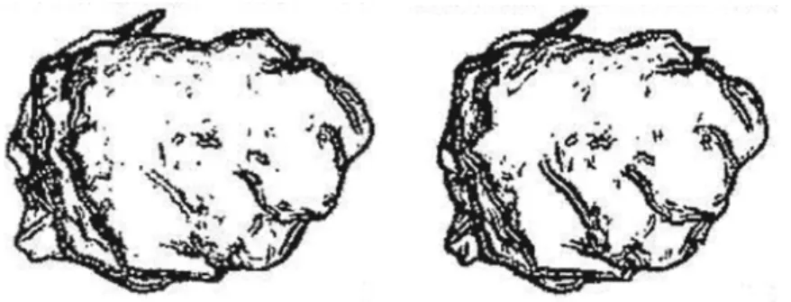
DIA instruments, on the other hand, picture particles falling from a vibrating tray or propelled by a fluid jet. The exact orientation of an individual particle in this configuration is never really known and it is certainly not reasonable to think that pure randomization is achieved. As a consequence, DIA image analysis provides a statistical distribution of diameters without being able to attribute them either to the exact length (a), width (b) or thickness (c) of any particle. Fig. 1 illustrates the difference of 2D imaging under controlled (SIA) or uncontrolled (DIA) particle orientation for rice grains.
In order to reconcile both imaging techniques and to make a definitive breakthrough in the characte-rization of individual particles, it makes no doubt that 3D imaging techniques are needed. Though still in their infancy and often poorly suited to analyse more than a few hundreds of particles within a single run, several 3D imaging techniques are now widely available. It is the intention of this paper to review a selection of techniques allowing for partial or full 3D imaging of particle surfaces (surfometry) or internal structures (tomography).
3D IMAGING AND SPATIAL SAMPLING
A particle is a solid body extending in three dimensions. In order to build a useful discrete representation of this body, we need a technique capable of probing any location within the particle or on the particle surface with a high enough spatial
density. As has been shown in 2D (Pirard and Dislaire, 2005), the adequate resolution for unbiased estimation depends on the desired geometrical feature and on the algorithm used to estimate it. A rough guess leads to a minimum of 100 elementary volume elements (voxels) for properly estimating the volume of a particle, a minimum of 1000 voxels for estimating aspect ratios and probably more than 104
voxels to estimate surface roughness and other high scale properties.
The 3D imaging of a single particle is thus a spatial sampling operation to which the following terminology applies:
- The field is the spatial extension completely enclo-sing the particle of interest. It relates to a notion commonly understood in imaging as magnification. - The sampling grid is the set of locations of all
volume elements (voxels) used to build the image. Theoretically it should be random to ascertain equiprobability, but in practice most instruments will follow a systematic arrangement of points or at least use a resampling procedure to yield such a systematic arrangement. This notion is commonly understood as the image grid, array or raster. - The sample support is the spatial extension upon
which a measurement is performed. It is the volume over which the property attributed to the voxel will be integrated. This notion corresponds to the usual concept of (spatial) resolution. The probing principle itself can be extremely diverse. In the broadest sense, it does not need to be an optical property but can be any measure derived from a sound physical principle. The physical sensing of the particle can be passive (ex. atomic force scopy) or active (ex. transmission electron micro-scopy), depending on whether or not an external excitation (illumination) is required.
Fig. 1. Four rice grains pictured under controlled orientation (a) and uncontrolled orientation (b).
But, whatever the imaging principle used and even with the highest sampling density (resolution), it is essential to keep in mind that sampling always induces a loss of information. This loss of information is more or less severe depending on the detection limit and sensitivity of the sensor. In particular, if the sensitivity is too low the particle will be poorly contrasted from its background (embodying medium) and the particle representation will be severely degraded after seg-mentation (binarisation) of the voxels.
RESOLUTION AND MAGNIFICATION
Existing 3D sensing techniques cover a very large range of field magnifications starting from a few nm³ in Transmission Electron Tomography and reaching several km² in LIDAR (Laser Intensity Detection and Ranging). As a consequence, a very wide selection of particles can theoretically be imaged in 3D. But, what is of critical importance in many applications is the dynamic of the imaging system. In other terms, its capability for simultaneously picturing the smallest and the largest particle within a widespread particle population. This is the result of the sampling density (resolution) achieved at a given magnification. It is often very much dependent upon the scanning speed and/or the intrinsic resolution of linear or matrix sensors.
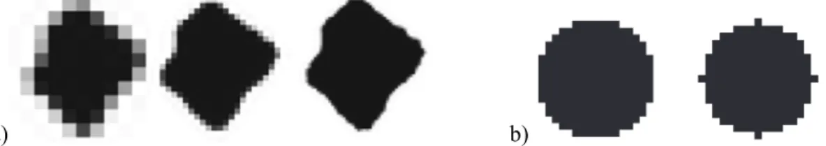
In practice, it is essential to distinguish the true resolution from the resolution achieved after resam-pling and (often undocumented) voxel interpolation. The simplest way to get a clear picture of the true resolution is thus to put a reticule or a standard product under the imager and check the results against the documented data. This is especially true for all systems where complex image reconstruction is required or where resolution is achieved by combining sensor resolution and mechanical resolution (Fig. 2).
In this review, we will focus on the most popular and promising techniques which yield good quality 3D pictures from most organic and inorganic solids at scales ranging from nanometres to decimetres.
SYSTEMATIC SAMPLING GRIDS
The literature on unbiased estimation of geomet-rical properties from discrete (square) sampling grids is still limited or at least poorly diffused among the naive users of image analysis (Dorst and Smeulders, 1987; Stoyan et al., 1995; Russ and de Hoff, 2000).
The definition of a grid suffices to represent an object with a digital image and allows for estimating its Lebesgue measure (area in 2D and volume in 3D). However, in order to address notions such as perimeter length or connectivity it is essential to complement it with an associated graph, defining how picture ele-ments have to be linked to each other. As shown in Fig. 3, the choice of a graph is nothing else but the choice of a model and it has a significant influence on the estimators, precluding any idea of comparing results gained from identical imaging systems using different graphs. The acquisition of information along a systematic grid in three dimensions is almost impo-ssible to achieve. The 3D sampling grid is in general made out of a series of parallel 2D sections whose spacing is not equivalent to the sampling interval within the section. Most often, be it through tomogra-phy or through mechanical slicing, the third dimension is less well sampled than the imaging plane. Hence δx = δy << δz. In order to perform image processing and image analysis, it is much more convenient to resample the 3D space and obtain a systematic 3D grid. This can be achieved using different interpolation methods, from nearest neighbour techniques to more elaborated topo-probabilistic inference (kriging). It has been shown by Meyer (1992) that the most evident 3D cubic grid is not especially the most convenient one for interpolation and that centred cubic (CC) grids and face centred cubic (FCC) grids present a lot of interest because they also allow for less biased image analysis measurements (Fig. 3b). The elementary nei-ghbourhood on such grids is defined as a cubocta-hedron (each pixel having twelve nearest neighbours) which is a shape closer to the sphere than the cube. As far as we know, this recommendation is not especially implemented in many softwares and a majority of them still use cubic neighbourhoods instead.
a) b)
Fig. 2. a) The same particle represented with different sampling grids (resolutions) in 2D. b) A disc-shaped
a) b)
Fig. 3. a) Partial drawing of the inner and outer perimeters of an object (black dots) in 8-connexity (plain
lines) or 4-connexity (dotted line); b) 3D grid obtained from a series of parallel 2D slices and corresponding cuboctahedral graph applied for neighbourhood operations after resampling into a systematic FCC (face centred-cubic) grid.
SURFOMETRIC IMAGING OF
PARTICLES
Under this section, we will review a series of technologies available to render the three dimensional topography of the outer envelope of a particle. Most technologies will only reveal that part of the surface directly visible to the sensor, but by combining views from different angles it is always theoretically possible, though often extremely tedious, to rebuild the full 3D surface.
Full 3D surfometric imaging from
projections
Probably the most obvious way to gain information about the three dimensions of an object is to picture it from different viewpoints and try to recombine the images or at least the measures performed in three or more planes. While it is relatively easy to rotate a large body and take pictures of it in a controlled geometric setting, this appears to be more cumbersome in microscopy. At macroscopic scale, the technique does not involve any specific imaging instruments but only a well-known geometrical arrangement of
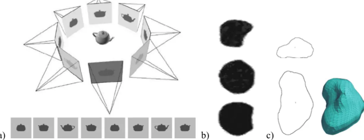
the light source, the body and the camera (Fig. 4). Reconstruction of the 3D object is not an easy task but it is widely discussed in computer vision. A good overview is given in Yemez and Schmitt (2004).
A special tri-axial setup has been designed by Yamamoto et al., (2002) for imaging particles of less than one millimetre. Their device uses three LEDs and two prisms to image a particle lying on a transparent rotating stage in three orthogonal planes. The authors did not try to recombine the profiles into a 3D image but attributed a triplet of orthogonal 2D measures to each particle. He (2010) used a similar principle to rebuild realistic 3D particle envelopes to feed his Discrete Element Models (DEM).
Some authors have tried to develop an industrial system based on the use of simultaneous images from different cameras (Bujak and Bottlinger, 2008). In this configuration, particles are pictured when falling one at a time in the centre of a ring formed by eight cameras. More recently Kempkes et al. (2010) developed a system to capture images of particles flowing between four glass plates using two ortho-gonal viewpoints.
a) b) c)
Fig. 4. a) Principle of imaging from multiple projections (Yemez and Schmitt, 2004). b) Three orthogonal
views of a single 800 µm particle (Yamamoto et al., 2002). c) Two orthogonal projections of an aggregate and its corresponding 3D meshing (He, 2010).
Partial 3D surfometric imaging
The reproduction of the (micro)topography of a surface is a major concern in many fields of techno-logy. It is of interest to tribologists who try to under-stand the role of surface roughness in mechanics, it is also essential to those who analyse the geomorphology of our planet and its impact on habitability. This means that similar software and hardware solutions are often to be found in unexpected fields of applications. Although very different sensing principles can be used, we will try to group together the imaging techniques sharing a similar scanning mode. Indeed, building the 3D image of a surface is possible using either a sweeping beam (whiskbroom imaging), a linescan camera (pushbroom imaging) or a classical staring array camera (raster imaging).
Whiskbroom surface imaging
Whiskbroom imaging builds an image of the surface point after point. This means that the image resolution is a compromise between integration timing (exposure) for each point and scanning rate. If a long integration timing is required because of poor sensi-tivity of the sensor, than obviously a reduced resolution will only be achieved at a constant scanning rate.
Mechanical scanning probe imaging
Profilometry or mechanical profiling of a surface with a stylus is very well known since decades and has long been considered in mechanics as the most reliable principle to gain information about a surface. It basically relies on direct contact between a tip and a surface. If the tip is regularly scanned along a series of parallel lines a complete surface image can be obtained. The digitizing frequency sets the horizontal resolution, whereas a stepping motor determines the
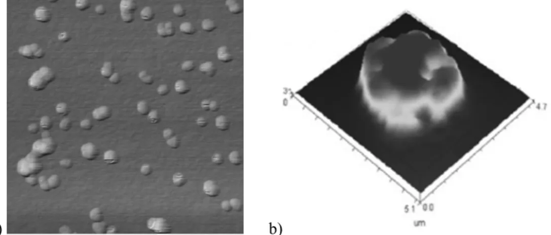
distance between two parallel profiles. Measurements in Z (altitude) are derived from a piezometric adjust-ment of the cantilever. The principle of mechanical profiling has been pushed to its limits in the family of scanning probe microscopes. In those systems, tips are claimed to be as small as a single atom (< 1 nm), thus allowing nanometric features to be identified. Both the movement of the tip and the interaction of the tip with the surface (ex. resistance; capacitance; tunnelling; etc.) can be registered. Nano-topography using such devices is very delicate and time consuming and since the scanning area is often a few tens of microns, it is only of practical interest for nanoparticle imaging where no other technique can compete (Fig. 5a). The sample preparation and above all the cleanliness of the surface are a big matter of concern. The vertical resolution in ideal conditions is below the angström, whereas lateral resolution can easily reach atomic resolution (Friedbacher et al., 1991; Rao et al., 2007; Starostina et al., 2008).
Optical scanning beam imaging
A simple principle in optics is that the light path depends upon the wavelength. Confocal microscopes take advantage of this principle by using a mono-chromatic laser beam illumination instead of conven-tional white light. As a result, the depth of focus or illuminated volume is much smaller and by inserting a pinhole in front of the detector it is possible to eliminate almost any excitation that is out of focus. In transparent materials such as biological tissues, a confocal microscope will perform optical slicing with 0.5 µm to 1.5 µm thickness. If such slices are acquired for a series of regularly spaced positions along the Z axis, a 3D image can be built. By stacking optical slices obtained from opaque samples, one gets a precise surfometric image of the scene with a typical
a) b)
Fig. 5. a) Topography of TiO2 nanoparticles on silicon (Rao et al., 2007). The height of the nanoparticles is in
the range of 10 nm, the total frame width is about 1 µm. b) Surface imaging of a 2.7 µm BSA (Bovine Serum Albumine) particle using white light interferometry (Adi et al., 2008)
lateral resolution of 200 nm for a vertical resolution in the order of 500 nm at best (Maire et al., 2011). Though very time consuming, this technology can be of particular interest when the laser light interaction (ex. Raman scattering) brings additional insight into the particle composition (Cherney and Harris, 2010).
The use of pulsed laser beams is an interesting alternative in that it allows building images using Light Detection and Ranging (designated under the acronym of LIDAR or sometimes LADAR). This technique is very popular in airborne instrumentation and also for industrial applications such as stockpile monitoring. It relies on the measure of the so-called time-of-flight of the laser light. Considering that a 1 ns delay is equivalent to a 15 cm distance, it is unlikely that this principle could efficiently compete with other principles at microscopic level. But, it is widely used in imaging at centimetric resolution. A good example relative to its application on aggregate monitoring is given in Garboczi et al. (2006).
The use of a scanning laser beam is also an inherent principle in imaging interferometers. These instruments are used to picture and analyse interference fringes produced by two beams travelling along optical paths that slightly differ in their length. A classical geometry is the Michelson interferometer which exploits the interference between a laser beam split into two different optical paths. The first one is sent towards a reference mirror while the second one is reflected by the sample surface. An interference figure with fringes separated by a distance of λ/2 (typ. 275 nm) is produced as soon as there is a difference in light path. As such, interferometers are rather time consuming instruments that deliver very high precision but are merely focussed towards the detection of the departure of a shape with respect to a reference surface. Therefore they are essentially suited to control manufactured surfaces for high-end applications (optics, electronics, etc.). Drawbacks of the interferometric technique include a very narrow field of view necessitating multiple acquisitions for millimetric sized objects and a very short working distance making it difficult to acquire images from distant surfaces (isolated by a vacuum box or a furnace window). For a recent example of using white-light interferometry in analysing surface roughness of micron sized particles, see Adi et al. (2008) (Fig. 5b).
Holographic imaging can also be considered as part of a similar technology. Again a reference monochromatic beam is split into two different light paths and interference is produced on the image plane between the beam reflected by a set of mirrors and the same beam reflected by the object. The
ad-vantage of such recording is that it is possible to reconstitute the image of the object when illuminating the image plate with the original reference beam.
Though still very heavy and time consuming, the principle of holographic imaging for analysing particle (plankton) size and shape in a one litre volume has been developed by Malkiel et al. (2004).
Pushbroom surface imaging
A pushbroom imager builds an image of the surface line by line. The resolution along the line (also called across track) is fixed by the performance of the sensor (linear camera) whereas the resolution perpen-dicular to it is fixed by the relative movement of the sensor with respect to the sample. It is often possible to determine the adequate sample speed to achieve equal resolution in both directions, but the limiting factor is the time required to reach optimal exposure of the sensor.
Imaging from triangulation
A classic example of pushbroom technology for 3D surfometric imaging is laser triangulation. In this technology, a laser plane is shed onto the surface. A conventional black and white video camera captures the image of the scene wherein the reflected laser beam appears as a broken line indicating the interaction with an irregular surface (Fig. 6). Knowing the geometry of the system (inclination of the camera with respect to the laser plane; typically 45°) it is straightforward from trigonometry to convert pixel positions into relative altitudes. Dedicated systems use specific hardware solutions to extract the reflected laser line and compute topography from triangulation, being capable to yield up to 35 000 profiles per second in optimal conditions. Reflectance (or colour) information is gathered from the same instrument and can be draped onto the shape for more realistic rendering. Most manufacturers have a range of similar instruments addressing different magnifications. Some however provide the user with interchangeable lenses. Typical scanning width are of the order of 50 mm, which represents an indicative spatial resolution of only 6 mm while the vertical resolution might be as good as 200 µm. Some systems provide magnifications up to 15 mm x 15 mm allowing to measure vertical variations down to 8 µm. The speckle effect accom-panying laser reflection on finely textured surfaces becomes problematic at higher magnifications and hinders precise measurements.
This technique has been used by Lanaro and Tolppanen (2002) for the analysis of individual aggre-gates (Fig. 7a). It has also been tested on over-lapping
aggregates and iron pellets by Thurley and Andersson (2007). At University of Liege, two optical benches using laser triangulation technology have been deve-loped. The first one is for very fine particles in the range 50 µm-1 mm (Fig. 7b) and the second one aims to analyse larger aggregates in the range 4 mm-100 mm.
Multifocus imaging
Raster surface imaging
Raster imaging modes generate all pixels of a 2D matrix simultaneously. Such imaging modes are available from staring array imagers which are best represented by the conventional CCD or CMOS sensors used in video imaging. The standard silicon sensors have a dynamic range in the visible part of the spectrum that can be digitized into 256 grey levels (8 bits), but scientific grade cooled silicon CCD might yield up to 4096 grey levels (12 bits).
Images taken with a video camera give no indica-tion of topography, but a subtle use of computerized imaging technologies has given way to a simple 3D surface imaging technology that can be designated as “multiple focus imaging”. The principle is somehow similar to confocal imaging in the sense that it takes advantage of the finite depth of focus of the scene but it uses white light instead of monochromatic laser beams.
A series of images are taken while the object is scanned in the Z axial direction (a stepping motor must be installed on the microscope column). These images are stacked together and after co-registration each pixel is analysed to identify in which section it did appear as the most in-focus. The simplest algo-rithms to determine the optimal focusing of a pixel compute the local grey-level variance around the pixel
Fig. 6. Principle of laser triangulation using a laser plane intersecting the object to be imaged. The known
geometry of the optical axis of a video camera allows for topographic information to be retrieved after automatic extraction of the laser line (in red) in the grey level image.
a) b)
Fig. 7. a) Full 3D image of an aggregate as obtained from laser triangulation of both faces (Image from
Illeström’s PhD thesis in Lanaro and Tolppanen, 2002). b) Image of 500 µm – 1 mm drill cuttings imaged by high-resolution laser triangulation (Limam et al., 2010)
and search for a maximum through the stack of images (Niederoest et al., 2004). This maximum should corres-pond to the best focus (where the most details are visible). However this technique can be very disap-pointing when no clear maximum of variance is reached. Many authors have proposed variants and there is a huge literature on the similar topic of auto-focusing. Some commercial instruments have rede-signed the hardware and use undisclosed algorithms to improve the results. Instrument stability and precise co-axiality between the mechanical axis and the optical axis are essential aspects for yielding good quality images. The technique does not require sample pre-paration and may give results comparable to confocal microscopy at a more affordable price. Due to the Z scanning and to the processing of typically 50 images it is almost as time consuming as confocal. It is not suited for transparent materials since in such cases the best focus point might be found in the very middle of the object and not on its outer surface. Such erratic results can be overcome by using image filtering techniques when the transparency is very local (outlier) but not when it dominates in the picture (Fig. 8). Typical performance is a maximum of 0.1 µm vertical resolution. The image stack covers a range between 500 µm and up to 2 mm with a typical acquisition time of 100 sec for a 150 images stack.
Structured light imaging
The principle of laser triangulation is very attrac-tive and convenient for a broad range of applications. Therefore it has been adapted in several ways depending on the constraints of the application. One of the most popular approaches consists in sending a series of parallel planes instead of a single plane. This is the so-called structured light imaging or Moiré imaging. The obvious advantage is that a rough volumetry can be obtained very quickly with no moving parts. Standard systems have been developed down to microscopic resolution claiming a lateral resolution of 8 µm at best and a corresponding depth resolution of less than 2 µm. Recently, impressive sub-diffraction resolution imaging has been developed thanks to 3D structured illumination microscopy (Schermelleh et al., 2008; Shao et al., 2008). Fig. 9 shows clusters of nanometric beads being resolved at 135 nm distance. As far as we know the technology has not yet been used to measure and characterize nanometric particles, but it appears very promising.
Fig. 8. 3D Images of a crushed limestone particle and
a transparent glass bead as obtained with a multi-focus imaging system (Alicona).
Fig. 9. A cluster of mixed red and green fluorescent
beads with 135nm centre-to-centre distance as seen in lateral and axial sections with the I5S 3D imaging principle (Shao et al., 2008).
Stereoscopic imaging
Our binocular vision takes advantage of the so-called parallax effect to gain a 3D impression of the world surrounding us. Using vision instruments, it is obviously possible to reproduce this effect and compute distance to sensor information for 3D modelling of the surface. Stereoscopic (or stereometric) imaging is now widely used for volumetry of objects from elec-tron microscopy to remote sensing (Tang et al, 2008). A major drawback of the technique is however the need for correlation between two images taken from different viewpoints. In other words, if the scene does not contain remarkable features that can be identified in both images, it is impossible to compute a parallax effect. In practice, unless the scene is heavily textured, it is unrealistic to expect a full automation of the procedure and a human operator has to sit behind the screen and click a series of control points in both images. In order to facilitate this procedure, it can be useful to apply a convolution filter (e.g Sobel) for computing local grey level gradients in the image (Fig. 10). SEM-based stereoscopy claims a vertical resolution down to 25 nm.
VOLUMETRIC IMAGING OF
PARTICLES
3D volumes from sections
Automated Serial Sectioning Tomography
A practical way of gaining 3D information is to cut the material into parallel slices and to rebuild the 3D image from the succession of 2D ones, following the Cavalieri principle. This is commonly done in stereo-logical analysis of biostereo-logical samples, but in material sciences precise sectioning of hard materials is a real issue and therefore a preferred approach is controlled grinding. The idea of removing a specific amount of material and taking pictures after each step is however extremely tedious and hard to control (Dinger and White, 1976). In order to appreciate the amount of
material removed after polishing, Chinga et al. (2004) used spherical beads. Others have tried using pyramidal microhardness imprints. Recent developments in fully automated material preparation have led to the deve-lopment of a dedicated robot. Spowart et al. (2003) illustrate the use of this instrumentation for imaging micron sized SiC particles in an aluminium matrix (Fig. 11). The typical slicing rate claimed by the RoboMet3D system is 5 to 20 slices per hour, with a slice thickness between 0.16 µm and 2.7 µm. Although extremely time consuming this method has the advantage over tomography techniques (see next paragraph) of being able to picture particles in a medium showing a poor contrast. It can also be associated to a series of microanalytical instruments to offer 3D imaging coupled to EDX and EBSD information for example (Uchic et al., 2011).
Automated serial sectioning is not the only me-thod to remove a controlled amount of material during polishing. Developments in ion beam milling techni-ques have led to the development of systems wherein a nanolayer of material is removed from the surface while being imaged with high resolution electron microscopy. This technique is known as dual-beam focused ion beam/scanning electron microscope (FIB/ SEM) and leads after 3D reconstruction of the slices to FIB Nanotomography (Fig. 12). Holzer et al. (2006) and Cao et al. (2009) have shown impressive examples of 3D nanoparticle shape analysis.
Optical and X Ray Micro Computed Tomography
A less destructive technique is tomography which can be achieved in any sufficiently transparent me-dium from a set of linear images taken from different viewpoints (typ. 400 per 180°). The linear sensor is than moved upwards (or the sample downwards) in order to scan the third dimension. With a few excep-tions, X-ray sources are needed in material sciences in order to be able to traverse the sample.
Fig. 10. Gradient images (Sobel filter) are efficient to improve the identification of control points in
Fig. 11. Surface rendering of a 3-D model of an
indi-vidual SiC particle, comprising 35 serial section slices. Spacing between slices = 0.16 ± 0.01 µm. (Spowart et al., 2003).
Fig. 12. 3D rendering of nanosized Ni4Ti3 particles
in a Ni50.8Ti49.2 volume of4x4x4 µm³ as imaged with
FIB-SEM (Cao et al., 2009).
Konagai et al. (1992) developed a Laser-Aided Tomography (LAT) technique that has been used by Matsushima et al. (2003) to picture broken glass particles. It requires particles to be transparent to the laser radiation and the immersion medium to be of similar refractive index… which is of course a very exceptional situation.
Since a few years, X-ray tomography has been made available both as a desktop imaging instrument (Sassov, 2000) and as a joint imaging resource at synchrotron radiation facilities (Baruchel et al., 2000). The first instrument relies on compact sealed X-ray microfocus tubes with a spot size of about 5 µm. Because they are polychromatic, these sources cannot be focussed using X-ray lenses and their typical resolu-tions are in the order of 400 nm to 1 µm (Masschaele
et al., 2007). However, recent developments utilizing
high resolution zone plate lenses have achieved resolutions as low as 50 nm (Jakubek et al., 2006;
Stearing et al., 2011). Synchrotron radiation facilities offer monochromatic X-ray sources that bring much brighter images at higher resolution. See Baruchel et
al. (2000) for a complete overview. Because
synchro-trons generate much higher fluxes, it means in practice that much faster scans are possible thereby more easily enabling dynamic scans of particulate systems.
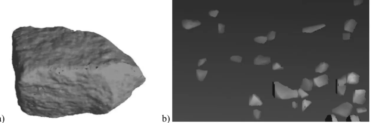
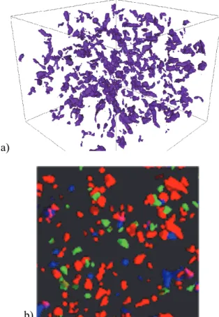
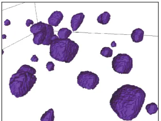
If X-ray tomography is performed on a single particle embedded in a light medium (e.g. wax, PVC powder) it allows to strongly contrast the outer surface which enhances the segmentation (particle extraction) procedure (Fig. 13). It should also be noted that X-ray tomography is unique in that it gives insight into the particle nature (density) and not only geometrical information, not to mention possibilities of data fusion from different microscopes and from X-ray fluores-cence (Latham et al., 2008; Miller et al., 2010).
Scanning transmission electron microscopy tomography
The interest of using electron beams instead of X-rays is that electron tomography will be able to achieve higher resolution even down to the atomic level
a)
b)
Fig. 13. a) 3D rendering of tortuous zinc particles (100
µm thick) imaged with a desktop system after dis-persion in a fine PVC powder. b) Visualisation of multiple phases (silicates, chromite and iron sulphi-des) within single particles from a platinum ore.
Fig. 14. STEM HAADF reconstruction of nanometric
ErSi inclusions in a ceramic body.
(Weyland and Midgley, 2004; Van Aert et al., 2011). The electron beam also generates images with a stronger contrast. Electron tomography is usually performed within a Scanning Transmission Electron Microscope (STEM) using a HAADF (High Angular Angle Dark Field) annular detector positioned in such way to receive the high angle diffracted electron beams. However, other modes like two-beam imaging are also possible (Hata et al., 2008). In order to gather information about the third dimension, the sample is tilted in more or less seventy directions depending upon the desired resolution. 3D images obtained with STEM HAADF tomography are shown in Fig. 14. Like for X-ray CT, particles must be dispersed and embedded in a transparent medium before being imaged.
Examples of nanoparticles characterization were recently presented by Sueda et al. (2010) and Kaneko
et al. (2007).
CONCLUDING REMARKS
3D imaging of individual particles has become in less than a decade a very realistic and powerful tech-nology. Even though, further instrumental develop-ments are required to reach high speed imaging capa-bilities and make it possible to rival with 2D image analysis instruments, it is clear that 3D characterization opens the way to some unique characterization possi-bilities.
The techniques reviewed in this paper cover a wide range of particle size and sensing principles. This indicates that there is no single technique emer-ging and that most probably a combination of sensors and sensing geometries will yield the best results. Fusion of 2D images (ex. elemental mapping) with
3D tomographies is a good example of emerging techniques with a lot of potential in the analysis of composite particles.
With 3D imaging becoming more and more widespread, it makes no doubt that standards for particles size and shape analysis will have to be adapted. It is the intention of the author to pursue this review with an in depth inventory of particle size and particle shape parameters in 3D.
ACKNOWLEDGEMENTS
The author would like to gratefully acknowledge the long-term support of IFPRI (International Fine Particle Research Institute) in helping to compile this literature review and in supporting the development of 3D imaging and image analysis tools for particulate systems.
The author is also very much indebted to Schaefer Technologies for making the Alicona Infinite Focus images and to the Fraunhofer institute for sharing their STEM HAADF high-resolution images.
Finally, the enthusiast cooperation of Dr Veerle Cnudde and Marijn Boone from the UGCT X-ray microCT imaging center in Gent is heartily acknow-ledged with the sincere wish to further develop a 3D expertise in geosciences.
REFERENCES
Adi S, Adi H, Chan HK, Young PM, Traini D, Yan R, et al. (2008). Scanning white-light interferometry as a novel technique to quantify the surface roughness of micron-sized particles for inhalation. Langmuir 24: 11307–12.
Baruchel J, Buffiere JY, Maire E, Merle P, Peix G (2000). X-ray Tomography in Materials Science. Paris, Hermes. Bujak B, Bottlinger M (2008). Three-dimensional measu-rement of particle shape. Part Part Syst Charact 25: 293–7.
Cao S, Tirry W, van den Broek W, Schryvers D (2009). Optimization of a FIB/SEM slice-and-view study of the 3D distribution of Ni4Ti3 precipitates in Ni–Ti. J Microsc 233:61–8.
Cherney DP, Harris JM (2010). Confocal Raman micro-scopy of optical-trapped particles in liquids. Ann Rev of Anal Chem 3:277-97.
Chinga G, Johnsen PO, Diserud O (2004). Controlled serial grinding for high-resolution three-dimensional reconstruction. J Microsc 214:13-21.
Dinger DR, White EW (1976). Analysis of polished sections as a method for the quantitative 3-D characterization of particulate materials. Scan Elec Microsc 3:409–15. Dorst L, SmeuldersAW (1987). Length estimators for digi-tized contours. Comp Vis Graph Im Proc 440:311–33.
Friedbacher G, Hansma PK, Ramli E, Stucky GD (1991). Imaging powders with the atomic force microscope: from biominerals to commercial materials. Science 253:1261–3.
Garboczi EJ, Cheok GS, Stone WC (2006). Using LADAR to characterize the 3-D shape of aggregates: Preliminary results. Cem Concr Res 36:1072–5.
Hata S, Kimura K, Gao H, Matsumura S, Doi M, Moritani T, et al. (2008). Electron tomography imaging and analysis of γ' and γ domains in Ni-based superalloys. Adv Mat 20:1905-1909.
He H (2010). Computational modelling of particle packing in concrete. PhD Thesis, TU Delft.
Holzer L, Muench B, Wegmann M, Gasser Ph, Flatt RJ (2006). FIB-nanotomography of particulate systems– Part I: Particle shape and topology of interfaces. J Am Ceram Soc 89:2577–85
Jakubek J, Holy T, Jakubek M, Vavrik D, Vykydal Z (2006). Experimental system for high resolution X-ray transmission radiography. Nucl Instr Meth Phys Res, Sect A: Accel Spectro Detect Assoc Equip 563: 278–81.
Kaneko K, Inoke K, Freitag B, Hungria AB, Midgley PA, Hansen Th, et al. (2007). Structural and morphological characterization of cerium oxide nanocrystals prepared by hydrothermal synthesis. Nano Letters 7-2:421-425. Kempkes M, Vetter V, Mazzotti M (2010). Measurement
of 3D particle size distributions by stereoscopic ima-ging. Chem Engng Sc 65:1362.
Konagai K, Tamura C, Rangelow P, Matsushima T (1992). Laser-Aided tomography: a tool for visualization of changes in the fabric of granular assemblage. Struct Eng / Earthquake Eng 9:193–201.
Lanaro F, Tolppanen P (2002). 3D characterization of coarse aggregates. Engng Geol 65:17-30.
Latham SJ, Varslot T, Sheppard A (2008). Automated registration for augmenting micro-CT 3D images. Anziam J 50:534–48.
Limam S, Califice A, Pena C, Pirard E, Detournay E (2010). 3D and 2D particle image analysis of rock chips generated by core scratch tests. Proc. World Congress on Particle Technology, Nürnberg.
Maire E, Persson Gulda M, Nakamura N, Jensen K, Margolis E, Friedsam C, et al. (2011). Three-dimensi-onal confocal microscopy study of boundaries between colloidal crystals. In: Proulx T. ed. Optical measure-ments, modeling, and metrology. 5. Proc. Ann. Conf. on Experimental and Applied Mechanics.
Malkiel E, Abras J, Katz J (2004). Automated scanning and measurements of particle distributions within a holographic reconstructed volume. Meas Sc Technol 15:601–12.
Masschaele B, Cnudde V, Dierick M, Jacobs P, Van Hoorebeke L, Vlassenbroeck J (2007). UGCT: New X-ray radiography and tomography facility. Nucl Instr Meth Phys Res, Sect A: Accel Spectro Detect Assoc Equip 580:266–9.
Matsushima T, Saomoto H, Matsumoto M, Toda K, Yamada Y (2003) Discrete element simulation of an assembly of irregularly shaped grains: quantitative com-parison with experiments. In: 16th ASCE Engineering-Mechanics Conference, Univ. Washington, Seattle. Meloy TP (1977). A hypothesis for morphological
charac-terization of particles and physiochemical properties. Powd Technol 16:233–53.
Meyer F (1992). Mathematical morphology: from two dimensions to three dimensions. J Microsc 165:5–28. Miller J (2010). Characterisation, analysis and simulation
of multiphase particulate systems using high-resolution microtomography (HRXMT). In: Proc XXV Int. Mi-neral Processing Congress, Brisbane.
Niederoest M, Niederoest J, Scucka J (2004). Shape from focus: fully automated 3D reconstruction and visuali-zation of microscopic objects. In: International Archives of the Photogrammetry, Remote Sensing and Spatial Information Sciences XXXIV.
Pirard E, Dislaire G (2005). Robustness of planar shape descriptors of particles. In: Proc. Int. Assoc. Mathe-matical Geology (IAMG), Toronto.
Podsiadlo P, Stachowiak GW (1997). Characterization of surface topography of wear particles by SEM stereo-scopy. Wear 206:39–52.
Rao A, Schoenenberger M, Gnecco E, Glatzel Th, Meyer E, Brändlin D, Scandella L (2007). Characterization of nanoparticles using Atomic Force Microscopy. J Phys:Conf Ser 61:971–6.
Russ JC, de Hoff R (2000). Practical Stereology, Plenum Press.
Sassov A (2000). State of art micro-CT: X-ray microscopy. In: Proc VI Int. Conference, Berkeley, California (USA). 515–20.
Schermelleh L, Carlton PM, Haase S, Shao L, Winoto L, Kner P, et al. (2008). Subdiffraction multicolor ima-ging of the nuclear periphery with 3D structured illu-mination microscopy. Science 320:1332–6.
Shao L, Isaac B, Uzawa S, Agard DA, Sedat JW, Gustafsson MG (2008). I5S: wide-field light micro-scopy with 100-nm-scale resolution in three dimen-sions. Biophys J 94:4971–83.
Shearing P, Bradley R, Gelb J, Tariq F, Withers P, Brandon N (2012). Exploring microstructural changes associated with oxidation in Ni–YSZ SOFC electrodes using high resolution X-ray computed tomography, Solid State Ionics 216:69–72.
Spowart J, Mullens H, Puchala T (2003). Collecting and analyzing microstructures in three dimensions: A fully automated approach. JOM 55:35-8.
Starostina N, Brodsky M, Prikhodko S, Hoo CM, Mecartney ML, West P (2008). AFM capabilities in characterization of particles and surfaces: from angstroms to microns. J Cosmet Sci 59:225–32.
Stoyan D, Kendall WS, Mecke J (1995). Stochastic geometry and its applications. Chichester, Wiley.
Sueda S, Yoshida K, Tanaka N (2010). Quantification of metallic nanoparticle morphology on TiO2 using HAADF-STEM tomography. Ultramicr 110:1120–7. Tang X, de Rooij MR, van Duynhoven J, van Breugel K
(2008). Dynamic volume change measurements of cereal materials by environmental scanning electron microscopy and videomicroscopy. J Microsc 230:100–7. Thurley M, Andersson T (2007). An industrial 3D vision
system for size measurement of iron ore green pellets using morphological image segmentation. Miner Engng 21:405–15.
Uchic M, Groeber M, Rollett A (2011). Automated serial sectioning methods for rapid collection of 3-D micro-structure data. JOM 63:25–9.
Van Aert S, Batenburg KJ, Rossel MD, Erni R, Van
Tendeloo G (2011). Three dimensional atomic imaging of nanoparticles. Nature 470:374–7.
Wadell HA (1933) Sphericity and roundness of rock particles. J Geology 41:310–31.
Weyland M, Midgley PA (2004). Electron tomography. Mat Today 7:32–40.
Yamamoto KI, Inoue T, Miyajima T, Doyama T, Sugimoto M (2002). Measurement and evaluation of three-di-mensional particle shape under constant particle orien-tation with a tri-axial viewer. Adv Powd Technol 13: 181–200.
Yemez Y, Schmitt F (2004). 3D reconstruction of real objects with high resolution shape and texture. Im Vis Comput 22:1137–53.