Estimation régionale des débits de crues par la méthode ANFIS

E

ANFIS

E

ANFIS

Par

Chang Shu

Taha B.M.J. Ouarda

Chaire en hydrologie statistique (Hydro-Québec / CRSNG) Chaire du Canada en estimation des variables hydrologiques

INRS-ETE, Université du Québec

490, rue de la Couronne (Québec), Canada G1K 9A9

Rapport de recherche N° R- 930

ISBN 978-2-89146-542-7

TABLE OF CONTENTS

TABLE OF CONTENTS... V LIST OF FIGURES... VII LIST OF TABLES...IX ABSTRACT ...XI

1. INTRODUCTION AND REVIEW... 1

2. ANFIS ... 7

2.1 Basic fuzzy terminology ... 7

2.2 ANFIS Architecture... 9

2.3 Parameter indentification using hybrid learning algorithm ... 12

2.4 Structure identification using subtractive Clustering... 14

3. STUDY AREA ... 17

4. IMPLEMENTATION... 21

5. EVALUATION METHOD... 23

6. METHODS FOR COMPARISON ... 25

6.1 Artificial Neural Networks ... 25

6.2 Nonlinear Regression... 26

7. RESULTS AND DISCUSSION... 29

8. CONCLUSIONS... 37

LIST OF FIGURES

Figure 1. Typical Gaussian membership functions... 9

Figure 2. Architecture of the ANFIS ... 10

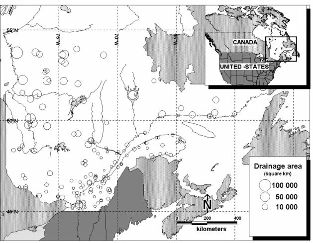
Figure 3. Hydrometric stations across the province of Quebec, Canada. ... 18

Figure 4. Scatter plot of site characteristics and flood quantiles ... 20

Figure 6. Jackknife estimation using the ANN approach ... 34

LIST OF TABLES

Table 1. Descriptive statistics of hydrological, physiographical and meteorological variables ... 19 Table 2. Cross-validation Results ... 29

ABSTRACT

In this paper, the methodology of using adaptive neuro-fuzzy inference systems (ANFIS) for flood quantile estimation at ungauged sites is presented. The proposed approach has the system identification and interpretability of fuzzy models and the learning capability of artificial neural networks (ANNs). The structure of the ANFIS is identified using the subtractive clustering algorithm. A hybrid learning algorithm consisting of back-propagation and least-squares estimation is used for system training. The ANFIS approach provides an integrated mechanism for identifying the hydrological regions, generating knowledge from the data, providing flood estimates and self-tuning to achieve the optimal performance. The proposed approach is applied to 151 catchments in the province of Quebec, Canada, and is compared to the ANN approach and the nonlinear regression (NLR) approach. A jackknife procedure is used for the evaluation of the performances of the two approaches. Results indicate that the ANFIS approach has a much better generalization capability than the NLR approach and is comparable to the ANN approach.

1. INTRODUCTION AND REVIEW

Providing reliable estimates of flood quantiles is essential for many engineering projects. However, it often happens that the record length of the available streamflow data at sites of interest is much shorter than the return period of interest, and even worse there may not be any streamflow record at these sites of interest. Regional flood frequency analysis can be used to construct more reliable flood quantile estimators in these situations. Hydrologic information from other member stations in a region is used to compensate for short records at these sites of interest.

The index flood method proposed by Dalrymple (1960) and the regional regression method are the two most used regional estimation procedures. In the index flood method, it is assumed that the distribution of flood peaks at different sites within a given flood regime is the same except for a scale parameter. Regression methods are frequently used to build models that predict flood quantiles as a function of site physiographical and other characteristics (Thomas and Benson 1970). The methods have been widely used to obtain flood quantile estimates at sites where no historical flood records are available (Zrinji and Burn, 1994; Hosking and Wallis, 1997; Pandey and Nguyen, 1999; Shu and Burn, 2004b; Ouarda, et al., 2006). The most used regression methods for regional flood quantile estimation are parametric regression approaches. By using these methods, the form of the functional relationship between the dependent and independent variables is assumed to be known but may contain parameters whose values can be estimated from the data set. A power-form equation is generally used to relate a flood quantile of interest to catchment

physiographic, geomorphologic and climatic characteristics. A logarithmic transformation is generally required to linearize this equation. The estimated flood quantile using this technique is unbiased in a logarithmic flow domain; however the estimation will be biased in real flow domain (McCuen et al., 1990). Pandy and Nguyen (1999) and Grover et al. (2002) compared different regression methods for flood quantile and index flood estimation at ungauged catchments. The dimensionless nonlinear model was identified as the best parameter identification method.

One of the most important and challenging steps in regional flood frequency analysis is the delineation of the homogeneous regions. Researchers have developed a number of regionalization techniques for objective determination of homogeneous regions (see e.g. Stedinger and Tasker, 1985; Acreman and Wiltshire, 1989; Burn, 1990; Hosking and Wallis, 1997; Reed and Robson, 1999; Ouarda et al., 2001; Chokmani and Ouarda, 2004; Shu and Burn, 2004a; Ouarda, et al., 2006). An extensive review and comparative evaluation of different regionalization techniques was conducted by GREHYS (1996a, 1996b).

During the past three decades, significant progress has been made in the two model free techniques, fuzzy logic and artificial neural networks (ANNs). These two techniques provide an attractive alternative to the traditional modeling tools. Fuzzy logic can easily incorporate expert knowledge into standard mathematical models in the form of a fuzzy inference system (FIS). A FIS is a nonlinear mapping of a given input vector to a scalar output vector by using fuzzy logic. A FIS simulates the process of human reasoning by allowing the computer to behave less precisely than conventional computing. It is suitable for approximate reasoning by using a collection of membership functions and

rules and is very powerful for modelling systems that are difficult to represent by an accurate mathematical model. Fuzzy systems have been widely used in solving problems in various areas and have also appeared in a number of applications in hydrology and water resources. The fields of hydrology and water resources commonly involve a system of concepts, principles, and methods for dealing with modes of reasoning that are approximate rather than exact. The capability of dealing with imprecision gives fuzzy logic great potential for hydrological analysis and water resources decision making (Bogardi et al., 2003). Fuzzy logic has been applied to solve problems in various domains in hydrology, such as hydrological extreme modelling (Pongracz, 1999; Shu and Burn, 2004a), hydrometeorological event classification (Bardossy et al., 1995), Groudwater flow and transport modelling (Bardossy and Disse, 1993; Dou et al., 1997, 1999; Woldt et al., 1997), and Pollutant transport in surface water modelling (Di Natale et al., 2000). An ANN is an information processing system with massive parallelism and high connectivity. It acquires and stores knowledge resembling biological neural networks of the human brain (Haykin, 1994). Most hydrological processes are highly nonlinear, time varying and spatially distributed. ANN models have the ability to learn the underlying relationship between inputs and outputs of a process from historical data without the physical rules being explicitly attached. Mathematically, an ANN may be treated as a universal approximator. ANNs have seen numerous applications in hydrology (Task Commite, 2000a, 2000b). In the domain of regional flood frequency analysis, they were introduced by Shu and Burn (2004b) for index flood and flood quantile estimation. The application to selected catchments in the United Kingdom (UK) indicates that the nonlinearity introduced by ANN models allows them to outperform multiple linear

regression methods. The generalization ability of a single ANN can be improved by using a properly designed ANN ensemble. Dawson et al. (2006) applied ANNs to flood quantile and index flood estimation for 870 catchments across the UK. The results obtained from the ANNs are comparable in accuracy with those obtain by the Flood Estimation Handbook (FEH) (Reed and Robson, 1999) models.

A judicious integration of fuzzy system and ANN can produce a functional neural fuzzy system capable of learning, high-level thinking, and reasoning (Loukas, 2001). It provides an effective approach for dealing with large imprecisely defined complex systems. Various schemes have been proposed for the integration. An adaptive neuro-fuzzy inference system (ANFIS) is one of the most successful schemes which combine the benefits of these two powerful paradigms into a single capsule (Jang, 1993; Jang, et al., 1997). An ANFIS works by applying neural learning rules to identify and tune the parameters and structure of a FIS. There are several features of the ANFIS which enable it to achieve great success in a wide range of scientific applications. The attractive features of an ANFIS include: easy to implement, fast and accurate learning, strong generalization abilities, excellent explanation facilities through fuzzy rules, and easy to incorporate both linguistic and numeric knowledge for problem solving (Jang, et al., 1997). Due to these fascinating features of the ANFIS, it is used in this paper to establish the relationship between catchment descriptors and flood estimates.

In this paper, the ANFIS is proposed to provide the regional flood estimation. This approach provides an integrated mechanism for identifying the hydrological regions, generating knowledge from the data, providing flood estimates and self-tuning to achieve the optimal performance.

Identifying homogeneous regions requires finding those sites that are similar in their hydrological response. This step is challenging due to the difficulty to derive the exact mathematical form to express the similarity between different catchments (Shu and Burn, 2004a). Furthermore, a trade-off between homogeneity and the size of a hydrological neighbourhood has to be taken into consideration (Ouarda et al., 2001). A small neighbourhood may ensure a high degree of homogeneity in the neighbourhood. However, it maybe very difficult to carry out an appropriate statistical estimation within the neighbourhood. Fuzzy techniques which are capable to model imprecision and uncertainty can be used to establish the relationships between the hydrological variable and physiogeographical variables by using fuzzy rules. There are generally two approaches to construct fuzzy rule bases. For the first approach, we might ask the domain experts to express their knowledge about the problem in the form of linguistic rules. This is the approach adopted by Shu and Burn (2004a) to derive the similarity between catchments that is subsequently used for homogeneous region delineation. In this approach, the fuzzy sets and fuzzy rules are initially specified by the domain experts and are tuned using optimization algorithms. For the second approach, the knowledge is generated directly from the observed field data. This approach is data driven, and thus is less subjective than the first one. The data-based approach is adopted in the present work. The subtractive clustering algorithm (Chiu, 1994) is used in the present work to identify the clusters of sites with similar physiogeographical characteristics. Rules representing the relationship between inputs and the output are then established based on the clusters. Parameters of the fuzzy system are adjusted during the training phase to achieve the best performance.

The goal of the ANFIS is to find a model or mapping that will correctly associate the inputs (catchment descriptors) with the output (flood statistics). By using the ANFIS approach, no (or very little) assumption is required about the form of the true function being estimated. In hydrology, the set of independent variables may be well defined, but the parametric form of the relationship is poorly understood. Thus, this type of nonparametric regression approach which makes no assumption concerning the form of the regression function has more advantages in this perspective compared to traditional parametric regression methods.

The remainder of this paper is organized as follows: In Section 2, a general introduction to the basic fuzzy terminology, the ANFIS architecture and the system identification is presented. In Section 3, a description of the study area is provided. In Section 4, details related to the implementation of the proposed approach are presented. In Section 5, the evaluation method is provided. In Section 6, the estimation models to be compared are presented. In Section 7, the results obtained by applying the proposed approaches are presented and discussed. Finally, in Section 8, the conclusions of this work are presented.

2. ANFIS

2.1 Basic fuzzy terminology

Fuzzy set theory was first developed by Zadeh (1965). It is primarily used to deal with uncertain and imprecise knowledge. It can be thought of as an extension of the traditional crisp set theory. Let A be a crisp set. A individual x from a universal set X is determined either to be a member of A or a non-member of A. This can be expressed by

( ) : {0,1}

A x X

μ → (1)

Crisp set theory using Boolean logic cannot be used to represent vague concepts such as the terms large, medium and small. This can be overcome by using fuzzy logic which extends the range of true values to all real numbers in the interval between 0 and 1. Fuzzy logic can be best understood using set membership where the membership values represent the degrees with which each object is associated with the properties that are distinctive to the collection. Formally, a fuzzy set A is defined as a collection of objects with membership values between 0 (complete exclusion) and 1 (complete membership). Membership grade of each element in X is determined through a membership function

A

μ which maps the elements of an universe of discourse X to the unit interval [0, 1], that is

: [0,1]

A X

By using approximate reasoning, a fuzzy logic description can be used to effectively model the uncertainty and nonlinearity of a system.

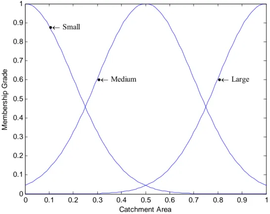
Suppose one of the input variables to a fuzzy system is the catchment area, and the value of the variable is translated into membership values of three fuzzy sets large, medimum, and small as displayed in Figure 1. The type of membership functions represented in Figure 1 is the Gaussian membership function. The Gaussian membership function has the following form:

2 2 1 ) , , ( ⎟⎠ ⎞ ⎜ ⎝ ⎛ − − = σ σ c x e c x Gaussian (3)

The function has two parameters c and σ . As the values of the parameters change, the membership functions vary accordingly, thus exhibiting various forms of membership functions. Other frequently used membership functions include triangular, trapezoidal and bell membership function.

0 0.1 0.2 0.3 0.4 0.5 0.6 0.7 0.8 0.9 1 0 0.1 0.2 0.3 0.4 0.5 0.6 0.7 0.8 0.9 1 •← Small •← Medium •← Large Catchment Area Me mb e rs h ip G ra d e

Figure 1. Typical Gaussian membership functions

2.2 ANFIS Architecture

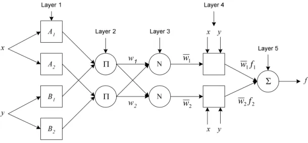
The proposed ANFIS model is a multilayer artificial neural network-based fuzzy system. A typical architecture of an ANFIS, in which a circle indicates a fixed node, whereas a square indicates an adaptive node, is shown in Figure 1. In this connectionist structure, the input and output nodes represent the catchment descriptors and the flood quantile, respectively, and in the hidden layers, there are nodes functioning as membership functions (MFs) and rules. This eliminates the disadvantage of a normal feedforward multilayer network, which is difficult for an observer to understand or to modify (Jang,

1993). For simplicity, we assume that the examined FIS has two inputs and one output. For a first-order Sugeno fuzzy model, a typical rule set with two fuzzy “if-then” rules can be expressed as follows:

Rule 1: If x is A1 and y is B1, then f₁ = p₁x+q₁y+r₁ (4)

Rule 2: If x is A2 and y is B2, then f₂ = p₂x+q₂y+r₂ (5)

where x and y are the two crisp inputs, and Ai and Bi are the linguistic labels associated with the node function. As indicated in Figure 2, the system has a total of five layers. The functioning of each layer is described as follows.

Π Π Σ 1 w 2 w 1 1f w 2 2f w

Figure 2. Architecture of the ANFIS

Layer 1: All the nodes in the first layer are adaptive nodes which means that the outputs

to a linguistic label which has a membership function i A μ or i B

μ . The output of a node in this layer specifies the degree to which the given input satisfies the membership function. The node function of a node i can be expressed by

) ( 1 x O i A i =μ , for i =l, 2 (6) ) ( 2 1 y O i B i =μ ₋ , for i =3, 4 (7)

In this paper, membership functions

i

A

μ and

i

B

μ are chosen to be Gaussian-shaped with maximum equal to 1 and minimum equal to 0. Parameters in this layer are referred to as premise parameters.

Layer 2: Nodes in this layer are labeled Π, whose output represents a firing strength of a

rule. The node generates the output (firing strength) by cross multiplying all the incoming signals: ) ( ) ( 2 y x w O i i B A i i = =μ ×μ , i = 1, 2. (8)

Layer 3: Every node in this layer is a fixed node labeled N. The ith node calculates the

ratio between the ith rule's firing strength to the sum of all rules' firing strengths:

2 1 3 w w w w O i i i + = = , i = 1, 2. (9)

Layer 4: Every node i in this layer is an adaptive node with a node function: ) ( 4 i i i i i i i w f w p x q y r O = = + + , (10)

where {pi, qi, ri} is the parameter set of this node. These parameters are referred to as consequent parameters.

Layer 5: The single node in this layer is a fixed node labeled Σ , which computes the

overall output by summing all incoming signals:

∑

∑

∑

There are two major phases for implementing the ANFIS for specific applications: the structure identification phase and the parameter identification phase. The structure identification phase involves finding a suitable number of fuzzy rules and fuzzy sets and a proper partition feature space. The parameter identification phase involves the adjustment of the premise and consequence parameters of the system. More detailed descriptions of the two phases are provided in the following two sections.

2.3 Parameter indentification using hybrid learning algorithm

the hybrid learning algorithm, which combines the least squares method (LSM) and the BP algorithm, is used to rapidly train and adapt the FIS. This algorithm converges much faster since it reduces the dimension of the search space of the original BP algorithm (Jang, 1993).

When the premise parameters are fixed, the overall output can be expressed as a linear combination of the consequent parameters. The output f can then be written as:

2 2 2 2 2 2 1 1 1 1 1 1 2 2 2 2 1 1 1 1 2 2 1 2 1 2 1 1 ) ( ) ( ) ( ) ( ) ( ) ( ) ( ) ( r w q y w p x w r w q y w p x w r y q x p w r y q x p w f w w w f w w w f + + + + + = + + + + + = + + + = (12)

Equation (12) is linear in the consequence parameters p1, q1, r1, p2, q2, and r2.

The hybrid learning algorithms of ANFIS consist of the following two parts (Jang, 1993): (a) the learning of the premise parameters by back-propagation and (b) the learning of the consequence parameters by least-squares estimation. In the forward pass of the hybrid learning algorithm, functional signals go forward untill layer 4 to calculate each node output. The nonlinear or premise parameters in the layer 2 remain fixed in this pass. The consequent parameters are identified by the least squares estimate. In the backward pass, the error rates propagate backward from the output end towards the input end, and the premise parameters are updated by the gradient descent. Jang, et al., (1997) provided the detailed description and the mathematical background of the hybrid learning algorithm.

2.4 Structure identification using subtractive Clustering

Defining the fuzzy sets and fuzzy rules is a necessary step in the design of fuzzy systems. If the training database is very large and data is of good quality and have good coverage of the feature space, using more linguistic labels to define the fuzzy sets and having more fuzzy rules will enable the fuzzy system to have better generalization capability. However, if the database is small, which is a common problem in flood frequency analysis, deriving a large rule base from the training data can easily overfit the system and cause it to lose the capability of generalization. Too many rules may also consume large computation time. Thus an effective partition of the input space is required to decrease the number of rules. The subtractive clustering algorithm (Chiu, 1994) is introduced in this paper to provide dimension reduction in the fuzzy system. The algorithm can be used to generate a fuzzy system with the minimum number of rules required to distinguish the fuzzy qualities associated with each of the clusters.

By using the subtractive clustering algorithm, the catchments in a study area can be divided into different clusters (hydrological regions). Thus each cluster exhibits certain characteristics of the system to be modeled. By projecting the clusters into the input space which is the physiographical space defined by the input variables, the antecedent part of the fuzzy rules can be defined. The consequent part of the fuzzy rules can then be estimated using the least-squares method (Chiu, 1994).

Subtractive clustering is based on a measure of the density of data points in the feature space (Chiu, 1994). The idea is to find regions in the feature space with high densities of data points. The point with the highest number of neighbours is selected as centre of the

cluster. The data points within a prespecified fuzzy radius are then removed, and the algorithm looks for a new point with the highest number of neighbours. This continues until all data points are examined.

Given a collection of n data points

{

}

∑

where the cluster radius ra is a positive constant. Thus, a data point that has many neighbouring data points will have a high potential of being a cluster center. The radius ra defines a neighbourhood. Data points outside this radius have little effect on the density measure. The choice of ra plays an important role in determining the number of clusters. Large values of ra will generate a limited number of clusters, while small values of ra will generate a large number of clusters.

After the density measure of each data point has been calculated, the first cluster center is chosen to be the data point with the highest density measure. Suppose x is the c₁ point selected and D is its density measure. Then, the density measure for each data c₁ point xi is revised by the formula

2 2 1 /(b/2) c i i r x x c i i D D e D = − − − (14)

where rb is a positive constant. Note that the data points near the first cluster center x c₁ will have significantly reduced density measures, so that they are unlikely to be selected as the next cluster center. The constant rb is usually greater than ra to prevent closely spaced cluster centers. Generally rb is specified as 1.5 times of ra. After the density measure for each data point is revised, the next cluster center

2

c

x is selected, and all of

the density measures for data points are revised again. A good stopping criterion developed by Chiu (1994) can be used to automatically determine the number of clusters.

3. STUDY AREA

The ANFIS approach has been applied to the hydrometric station network of southern Quebec, Canada. Hydrometric stations meeting the following three criteria are selected:

(1) To get reliable at-site estimation, a historical flood record of 15 years or longer is required.

(2) The gauged river should present a natural flow regime.

(3) The historical data at the gauging stations must pass the tests of homogeneity, stationarity and independence.

The number of selected stations is 151. They are located between 45°N and 55°N. The area of these catchments ranges from 200 2

km to 100000 km . The locations of these 2

Figure 3. Hydrometric stations across the province of Quebec, Canada.

Three types of data, physiographical, meteorological, and hydrological data are used in this study. The physiographical and hydrological data were extracted from the ministry of the environment of Quebec (MENVIQ) hydrological database and from the topographic digital maps of Quebec. Meteorological variables were obtained using interpolated historical data from the MENVIQ meteorological network across the province of Quebec.

Five variables including three physiographical variables and two meteorological variables are selected in this work based on the previous study by Chokmani and Ouarda (2004). The three physiographical variables are area, mean basin slope (MBS), and the fraction of

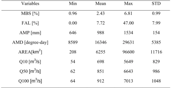
the basin area covered with lakes (FAL). And the two meteorological variables are annual mean total precipitations (AMP) and annual mean degree-days over 0°C (AMD). The summary statistics of these variables are presented in Table 1.

Table 1. Descriptive statistics of hydrological, physiographical and meteorological variables

Variables Min Mean Max STD

MBS [%] 0.96 2.43 6.81 0.99 FAL [%] 0.00 7.72 47.00 7.99 AMP [mm] 646 988 1534 154 AMD [degree-day] 8589 16346 29631 5385 AREA[km2_{] 208 6255 96600 11716} Q10 [m3_{/s] 54 698 5649 829} Q50 [m3_{/s] 62 851 6643 986} Q100 [m3 /s] 64 912 7013 1048

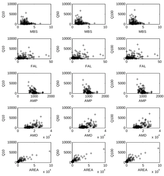
At-site flood quantile estimation for all the gauging stations in the study area was extracted from the database compiled by Kouider et al. (2002). For each site, the most appropriate statistical distribution was identified and fitted to the historical record to estimate at-site flood quantiles for a number of different return periods. The scatter plots between the quantiles and the selected physiographical and meteorological variables are shown in Figure 4.

0 5 10 0 5000 10000 MBS Q1 0 0 50 0 5000 10000 FAL Q1 0 0 1000 2000 0 5000 10000 AMP Q1 0 0 2 4 x 104 0 5000 10000 AMD Q1 0 0 5 10 x 104 0 5000 10000 AREA Q1 0 0 5 10 0 5000 10000 MBS Q5 0 0 50 0 5000 10000 FAL Q5 0 0 1000 2000 0 5000 10000 AMP Q5 0 0 2 4 x 104 0 5000 10000 AMD Q5 0 0 5 10 x 104 0 5000 10000 AREA Q5 0 0 5 10 0 5000 10000 MBS Q 100 0 50 0 5000 10000 FAL Q 100 0 1000 2000 0 5000 10000 AMP Q 100 0 2 4 x 104 0 5000 10000 AMD Q 100 0 5 10 x 104 0 5000 10000 AREA Q100

4. IMPLEMENTATION

The ANFIS is simulated using the Matlab Fuzzy Logic Toolbox. The initial parameters of the ANFIS are identified using the subtractive clustering method. However, the parameters of the subtractive clustering algorithm still need to be specified. The clustering radius is the most important parameter in the subtractive clustering algorithm and is optimally determined through a trial and error procedure. By varying the clustering radius ra between 0.1 and 1 with a step size of 0.01, the optimal parameters are sought by minimizing the root mean squared error obtained on a representative validation set. Clustering radius rb is selected as 1.5 ra. Default values are used for other parameters in the subtractive clustering algorithm.

Gaussian membership functions are used for each fuzzy set in the fuzzy system. The number of membership functions and fuzzy rules required for a particular ANFIS is determined through the subtractive clustering algorithm. Parameters of the Gaussian membership function are optimally determined using the hybrid learning algorithm. Each ANFIS is trained for 100 epochs.

5. EVALUATION METHOD

To assess the performance of each regional flood frequency analysis model, the following five indices are used: the Nash criterion (NASH), the root mean squared error (RMSE), the relative root mean squared error (RMSEr), the mean bias (BIAS), and the relative mean bias (BIASr). The indices are computed according to the following equations:

∑

∑

∑

∑

∑

∑

where n is the total number of sites being modeled, q is the at-site estimation for site i, i

i

qˆ is the estimation obtained from the regional flood frequency model for site i, and q is

The jackknife cross-validation procedure is used to assess the model performance. In this procedure, for each catchment in the study area, its flood records are temporarily removed from the database, thus it is assumed to be “ungauged”. Then each regional flood frequency analysis model is calibrated using the data of the remaining sites. Regional estimates can be obtained for the “ungauged site” using the calibrated models. They are then evaluated against its at-site estimates.

6. METHODS FOR COMPARISON

Aside from the ANFIS method, two other approaches are considered in this paper : the artificial neural networks and the nonlinear regression method. Both approaches treat the entire study area as a hydrological region.

6.1 Artificial Neural Networks

In this paper, the Multilayer perceptron (MLP) ANN model is selected to model the relationship between flood quantiles and catchment descriptors. MLP represents the most commonly used and well researched class of ANNs in hydrology and many other domains. The actual MLP adopted in this paper consists of an input layer, one hidden layer, and an output layer. The input layer accepts values of the input variables. The output layer provides the estimation. Layers lying between the input and output layer are called hidden layers. Based on the performance on a representative validation set, five neurons are used in the hidden layer of the ANN. The tan-sigmoid transfer function is used in the hidden layer and the linear transfer function is used in the output layer. Inputs (catchment descriptors) are standardized before feeding to the ANNs. A log transformation is used for the output (flood quantiles) of the ANN. The Levenberg-Marquardt algorithm (Hagan and Menhaj, 1994) is used for ANN training. This algorithm is more efficient than the basic back propagation (BP) algorithm. The regularization technique (Bishop, 1995) which penalizes model complexity is used to stop the ANN

training. Readers are suggested to refer to Shu and Burn (2004) for more detailed information on the model structure and training algorithm of the ANN model.

6.2 Nonlinear Regression

Parametric regression methods have been widely used for obtaining regional flood estimates. By using these methods, the relationship between the flood quantile QT and the catchment characteristics are assumed to be the power-form function (Thomas and Benson, 1970) which has the following form:

3 1 2

1 2 3 n

T n

Q =ax xθ θ xθ _Kxθ ...(20)

where θ_iis the ith model parameter, a is the multiplicative error term and n is the number of catchment characteristics.

Solving equation (20) using linear regression techniques generally requires linearizing the power-form model by a logarithmic transformation to the form. However, the estimation of the linearized model is theoretically unbiased in the logarithmic domain, but will be biased in the real flow domain (McCuen et al., 1990). Using nonlinear regression (NLR) methods, model parameters can be directly estimated by minimizing the estimation error in the actual flow domain. Nonlinear regression, with a properly selected objective function, can generally provide more accurate estimates than linear regression (Pandey and Nguyen, 1999; Grover et al., 2002).

In this paper, the NLR method is selected to compare with the proposed ANFIS approach. The objective function of the NLR is selected to minimize the difference between the observed and predicted flow as suggested by Grover et al. (2002)

∑

7. RESULTS AND DISCUSSION

The ANFIS approach proposed in this paper, the ANN approach and the NLR approach used for comparison purposes are applied to the study area database. The results obtained using the jackknife validation procedure are presented in Table 2.

Table 2. Cross-validation Results

Hydrological variables ANFIS ANN NLR NASH q10 0.85 0.83 0.79 q50 0.83 0.81 0.77 q100 0.82 0.80 0.75 RMSE [m3/s.km2] q10 316 338 377 q50 396 423 475 q100 437 463 520 RMSEr [%] q10 57 53 61 q50 62 58 67 q100 64 60 70 BIAS [m3/s.km2] q10 18 57 28 q50 20 59 34 q100 20 75 36 BIASr [%] q10 -8 -8 -9 q50 -12 -9 -11 q100 -14 -10 -12

The three models are evaluated based on the five indices described in Section 5. The

NASH values close to 0.8 are generally acceptable, while models with NASH values close

to 1 are deemed to produce near perfect estimation. The NASH values for the ANFIS and ANN models are all over 0.8 which indicates that both types of models achieved acceptable results. The NASH values of the ANFIS model are higher than those of the ANN model, which indicates that the overall quality of estimation of the ANFIS model is better than the ANN model. The NASH values for the NLR model are significantly lower than those obtained by the ANFIS and ANN models. The NASH values for the NLR model are all below 0.8 which indicates that quantile estimates obtained using the NLR model are of poor quality.

The prediction accuracy of a model in absolute and relative scale is assessed using RMSE and RMSEr respectively. The RMSE of the estimates computed by the ANFIS model is the lowest among three models. However the RMSEr of the ANFIS model is larger than those computed using the ANN model. Both the ANFIS and ANN models are showing better performances in these two indices than the NLR model.

The magnitude of systematic overestimation or underestimation of a model is evaluated using the BIAS and BIASr indices. The BIAS index provides the evaluation in the absolute scale. The results indicate that the three models generally overestimate flood quantiles. Based on the BIAS index, the ANFIS model is the least biased model, while the ANN is the most biased model. The BIASr index provides the measurement of bias in the relative scale; the results indicate that the three models generally underestimate flood quantiles. Based on the BIASr index, the ANN model is the least biased model, and the ANFIS and NLR have slightly higher biases than the ANN model.

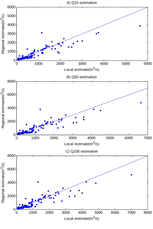
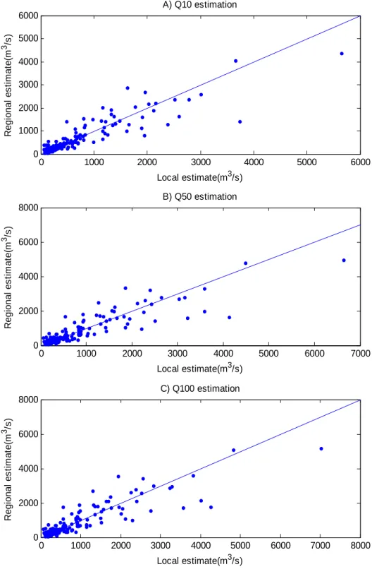
The regional estimates using the jackknife validation procedure for flood quantiles Q10, Q50, Q100 using the ANFIS, ANN and NLR methods are shown in Figure 5, Figure 6 and Figure 7 respectively. From these figures, we can observe that the estimation error and bias tend to increase with the return period. All models tend to provide less biased estimates for the sites with Q10 below 2200 m3/s, Q50 below 2500 m3/s and Q100 below 3000 m3/s. However, for sites with Q10 over 2200 m3/s, Q50 over 2500 m3/s and Q100 over 3000 m3/s, all three models tend to underestimate their flood quantiles. These sites represent the sites with the largest basin areas in the study area. The number of these sites accounts only for about 5% of the total sites, while the range of flood quantiles of these sites occupies the top 60% of the entire range of flood quantiles at the study area. Thus, correctly estimating these sites requires models with strong extrapolation capabilities. Nonparametric models like the ANFIS model and the ANN model are known to have a good descriptive ability but a limited predictive capacity (extrapolation).

The overall performance of the ANFIS model is better than the ANN model at larger sites, however the ANFIS model underperforms the ANN model for a number of sites with flood quantiles under 1000 m3/s. This is mainly due to the choice of clustering radius ra. Estimates of the flood quantiles at these sites can be significantly improved if ra

is reduced to around 0.56, however the best overall performance of the ANFIS model can be found if ra is in the range [0.68, 0.72].

The outperformance of the ANFIS approach over the NLR can be explained by the following two aspects. First, the ANFIS approach is capable to capture the feature of each individual hydrological region in the study area, while the NLR method treats the whole study area as a large hydrological region. The subtractive clustering algorithm used in the

ANFIS approach can identify a number of initial clusters (regions) and fuzzy rules that are used to capture the feature of each hydrological region. These clusters and rules are adjusted during the ANFIS training phase to improve the system performance. Second, the ANFIS approach requires no assumption on the underlying function. This provides the system the flexibility to approximate any arbitrary functions that may exist in the feature space.

0 1000 2000 3000 4000 5000 6000 0 1000 2000 3000 4000 5000 6000 Local estimate(m3/s) R egi onal e s ti m a te (m 3 /s ) A) Q10 estimation 0 1000 2000 3000 4000 5000 6000 7000 0 2000 4000 6000 8000 Local estimate(m3/s) R egi onal es ti m a te (m 3 /s ) B) Q50 estimation 0 1000 2000 3000 4000 5000 6000 7000 8000 0 2000 4000 6000 8000 Local estimate(m3/s) R e gi on al es ti m a te (m 3 /s ) C) Q100 estimation Figure 5. Jackknife estimation using the ANFIS approach

0 1000 2000 3000 4000 5000 6000 0 1000 2000 3000 4000 5000 6000 Local estimate(m3/s) R egi on al e s ti m a te (m 3 /s ) A) Q10 estimation 0 1000 2000 3000 4000 5000 6000 7000 0 2000 4000 6000 8000 Local estimate(m3/s) R egi on al es ti m a te (m 3 /s ) B) Q50 estimation 0 1000 2000 3000 4000 5000 6000 7000 8000 0 2000 4000 6000 8000 Local estimate(m3/s) R e gi ona l es ti m a te (m 3 /s ) C) Q100 estimation

0 1000 2000 3000 4000 5000 6000 0 1000 2000 3000 4000 5000 6000 Local estimate(m3/s) R egi o nal e s ti m a te (m 3 /s ) A) Q10 estimation 0 1000 2000 3000 4000 5000 6000 7000 0 2000 4000 6000 8000 Local estimate(m3/s) R egi ona l es ti m a te (m 3 /s ) B) Q50 estimation 0 1000 2000 3000 4000 5000 6000 7000 8000 0 2000 4000 6000 8000 Local estimate(m3/s) R e gi o nal e s ti m a te (m 3 /s ) C) Q100 estimation

8. CONCLUSIONS

In this paper, the methodology of using ANFIS for flood quantile estimation at ungauged sites is presented. The ANFIS approach provides a mechanism for integrating the two major steps, regionalization and estimation, in the regional flood frequency analysis into one system. Fuzzy rules and fuzzy sets in the ANFIS capture and store the regional information. The training algorithm tunes the system parameters over the entire data space according to the hybrid learning rules. Thus sharing and exchanging information between different hydrological regions are possible during the learning phase. This capability to model the interaction between different hydrological regions is one of the major advantages of the ANFIS approach over the traditional regional flood frequency analysis procedures where the regions once formed are mutually exclusive in the flood estimation step.

The ANFIS approach provides a general framework that combines two techniques, the ANNs and fuzzy systems. The ANFIS model provides nonlinear modeling capability and requires no assumption of the underlying model. By utilizing the fuzzy techniques, the linguistic relationship between the input and output can be expressed using the fuzzy rules. Unlike the initialization of an ANN, which may require several rounds of random selection, the initialization of an ANFIS can be performed using the one pass subtractive clustering algorithm. Through the ANN training, the ANFIS model tends to obtain missing fuzzy rules by drawing conclusions through the extrapolation of existing data. These rules could be unrealistic or simply untrue, and thus lead to inaccurate estimation.

A possible solution for this problem could be to supplement the fuzzy rule base obtained from observed data with rules specified by domain experts.

REFERENCES

Acreman, M. C., Wiltshire, S. E., 1989. The regions are dead; long live the regions. Methods of identifying and dispensing with regions for flood frequency analysis. IAHS Publication

no. 187, pp. 175-188.

Bardossy A., Disse, M., 1993. Fuzzy rule-based models for infiltration. Water Resources

Research, Vol. 29(2), pp. 373-382.

Bardossy, A., Duckstein, L., Bogardi, I., 1995. Fuzzy rule-based classification of circulation patterns for precipitation events. International Journal of Climatology, Vol. 15, pp. 1087-1097.

Bishop, C. M., 1995. Neural Networks for Pattern Recognition. New York: Oxford.

Bogardi, I., Bardossy, A., Duckstein, L., Pongrácz R., 2003. Fuzzy logic in hydrology and water resources. In: Fuzzy Logic in Geology, edited by: Demicco, R. V. and Klir, G. J., Elsevier Academic Press, pp. 153-190.

Burn, D. H., 1990. An appraisal of the 'region of influence' approach to flood frequency analysis.

Hydrological Sciences Journal, Vol. 35(2), pp. 149-165.

Chiu, S., 1994. Fuzzy Model Identification Based on Cluster Estimation. J. of Intelligent and

Fuzzy Systems. 2, 762-767.

Chokmani, K., Ouarda, T. B. M. J., 2004. Physiographical space-based kriging for regional flood frequency estimation at ungauged sites. Water Resources Research, Vol. 40(12): Art. No. W12514.

Dalrymple, T., 1960. Flood-frequency analyses. U.S. Geological Survey Water-Supply Paper

1543-A.

Dawson, C. W., Abrahart, R. J., Shamseldin, A. Y., Wilby, R. L., 2006. Flood estimation at ungauged sites using artificial neural networks. Journal of Hydrology, Vol. 319, 391-409. Di Natale, M., Duckstein, L., Pasanisi, A., 2000. Forecasting pollutants transport in river by a

fuzzy rule-based model. In: Workshop on Fuzzy Logic and Applications, Mons Institute of Technology, Belgium.

Dou, C., Woldt, W., Bogardi, I., 1999. Fuzzy rule-based approach to describe solute transport in the unsaturated zone. Journal of Hydrology, Vol. 220, pp. 74-85.

Eaton, B., Church, M., Ham, D., 2002. Scaling and regionalization of flood flows in British Columbia, Canada. Hydrol. Processes, Vol. 16, pp. 3245–3263

GREHYS, 1996a. Presentation and review of some methods for regional flood frequency analysis. Journal of Hydrology, Vol. 186, pp. 63-84

GREHYS, 1996b. Inter-comparaison of regional flood frequency procedures for Canadian rivers.

Journal of Hydrology, Vol. 186, pp. 85-103.

Grover, P. L., Burn, D. H., Cunderlik, J. M., 2002. A comparison of index flood estimation procedures for ungauged catchments. Canadian Journal of Civil Engineering. Vol 29, pp. 734-741.

Hagan, M. T., Menhaj, M., 1994. Training feedforward networks with the Marquardt algorithm.

IEEE Transactions on Neural Networks, Vol. 5(6), pp. 989-993.

Haykin, S., 1994. Neural Networks - a Comprehensive Foundation. Macmillan College Publishing, New York, NY, 852 pages.

Hosking, J.R.M., Wallis, J.R., 1997. Regional Frequency Analysis: An Approach Based on

L-moments. Cambridge University Press, New York, NY, 224 pages.

Jang, J. S. R., 1993. ANFIS: adaptive-network-based fuzzy inference system, IEEE Trans. Syst.,

Man Cyber. 23 (3) 665–685.

Jang, J. S. R., Sun, C. T., Mizutani, E., 1997. Neuro-Fuzzy and soft computing, Prentice-Hall: Englewood Cliffs, NJ.

Kouider, A., Gingras, H., Ouarda, T. B. M. J., Ristic-Rudolf, Z., Bobée, B., 2002. Analyse fréquentielle locale et régionale et cartographie des crues au Québec, Rep. R-627-el, INRS-ETE, Ste-Foy, Canada.

Loukas, Y. L., 2001. Adaptive neuro-fuzzy inference system: an instant and architecture-free predictor for improved. QSAR studies J. Med. Chem. 44 2772–2783.

McCuen R. H., Leahy R. B., Johnson P. A., 1990. Problems with logarithmic transformations in regression. Journal of Hydraulic Engineering, Vol. 116(3), pp. 414-428.

Ouarda, T. B. M. J., Haché, M., Bruneau, P., Bobée, B., 2000. Regional Flood peak and volume estimation in a northern Canadian Basin. ASCE Journal of Cold Regions Engineering, Vol. 14, pp. 176-191.

Ouarda, T. B. M. J., Girard, C., Cavadias. G. S., Bobée, B., 2001. Regional flood frequency estimation with canonical correlation analysis. Journal of Hydrology, Vol. 254, pp. 157-173.

Ouarda, T. B. M. J., Cunderlik, J. M., St-Hilaire, A., Barbet, M., Bruneau, P., Bobée, B., 2006. Data-based comparison of seasonality-based regional flood frequency methods. Journal

Pandey, G.R., Nguyen, V.-T.-V., 1999. A comparative study of regression based methods in regional flood frequency analysis. Journal of Hydrology, Vol. 225, pp. 92-101.

Pongracz, R., Bartholy, J., Bogardi, I., 2001. Physics and chemistry of the earth, Part B.

Hydrology, Oceans and Atmosphere, Vol. 26(9), pp. 663-667.

Reed, D. W., Robson, A. J., 1999. Flood Estimation Handbook, vol. 3. Institute of Hydrology, Wallingford, UK.

Shu C., Burn D. H., 2004a. Homogeneous pooling group delineation for flood frequency analysis using a fuzzy expert system with genetic enhancement. Journal of Hydrology, Vol. 291, pp. 132-149.

Shu C., Burn D. H., 2004b. Artificial neural network ensembles and their application in pooled flood frequency analysis. Water Resources Research, Vol. 40 (9): Art. No. W09301. Stedinger, J. R., Tasker, G. D., 1985. Regional hydrologic analysis 1. Water Resources Research,

Vol. 21(9), pp. 1421-1432.

Task Committee Report on Artificial Neural Networks in Hydrology, 2000a. Artificial neural networks in hydrology. I: Preliminary Concepts. Journal of Hydrologic Engineering, Vol. 5(2), pp. 115-123.

Task Committee Report on Artificial Neural Networks in Hydrology, 2000b. Artificial neural networks in hydrology. II. Hydrologic Applications. Journal of Hydrologic Engineering, Vol. 5(2), pp. 124-137.

Thomas, D. M., Benson, M. A., 1970. Generalization of streamflow characteristics from

drainage-basin characteristics, US Geological Survey, Water Supply Paper, 1975.

Wiltshire, S. E., 1986. Regional flood frequency analysis I: Homogeneity Statistics.

Hydrological Sciences Journal, Vol. 31(3), pp. 321-333.

Zrinji, Z., Burn, D. H., 1994. Flood frequency analysis for unguaged sites using a region of influence approach. Journal of Hydrology, Vol. 153, pp. 1-21.